Abstract
Low-latency data processing is essential for wide-area monitoring of smart grids. Distributed and local data processing is a promising approach for enabling low-latency requirements and avoiding the large overhead of transferring large volumes of time-sensitive data to central processing units. State estimation in power systems is one of the key functions in wide-area monitoring, which can greatly benefit from distributed data processing and improve real-time system monitoring. In this paper, data-driven Kalman filters have been used for multi-area distributed state estimation. The presented state estimation approaches are data-driven and model-independent. The design phase is offline and involves modeling multivariate time-series measurements from PMUs using linear and non-linear system identification techniques. The measurements of the phase angle, voltage, reactive and real power are used for next-step prediction of the state of the buses. The performance of the presented data-driven, distributed state estimation techniques are evaluated for various numbers of regions and modes of information sharing on the IEEE 118 test case system.
1. Introduction
State estimation in smart grids is regarded as an essential part of the energy management system (EMS) that enables wide-area monitoring of the system. The performance of the state estimation affects many critical functions of smart grids. However, inaccurate or unavailable system models can challenge conventional power system state estimation. As such, data-driven state estimation techniques have been pursued to complement conventional approaches by exploiting the large volume of available energy data. The data-driven approaches can also face challenges due to data communication and processing delays as well as missing or inaccurate data due to, for instance, measurement/sensor failures and cyber threats. Hence, developing effective mechanisms to improve the state estimation and the related communication and computation delays and enabling the recovery of missing information is crucial for enhancing the power system’s reliability and security.
Various data-driven state estimation approaches for smart grids have been proposed and studied in the literature [1,2,3,4,5,6], most of which are centralized techniques [1,2,4,5,6]. Real-time wide-area monitoring of smart grids demands low-latency data processing. Traditionally, a lot of data processing and calculations linked to power system monitoring have been carried out centrally on servers or cloud platforms owned by utilities. The vast volume of data that must be transmitted and processed in centralized locations necessarily causes delays and errors in system state estimation and monitoring. Such delays may have an impact on the stability and reliability of the system for some time-sensitive functions. Distributed and local data processing strategies are promising and can enhance system monitoring capabilities by enabling low-latency requirements and avoiding the enormous overhead of transmitting a large volume of time-sensitive data to central processing units. Examples of distributed state estimation studies include [3,7,8], where the state estimation has been implemented using various machine learning-based frameworks. This paper studies multiple distributed data-driven state estimation techniques under various scenarios of information sharing among distributed areas. It is demonstrated that multi-area distributed state estimations can speed up the system’s reaction time, especially in response to urgent situations such as failures or cyber stressors [3]. With the help of local and distributed data processing in power grids, new technologies, such as edge or fog computing, can enable these functions [9].
Specifically, in this paper, interpretable and generalizable data-driven approaches for state estimation based on Kalman filters in multi-area settings are studied. Both linear and non-linear Kalman filters, particularly extended and unscented Kalman filters, with data-driven models to approximate the power system dynamics, are considered in a wide range of scenarios, including centralized, fully distributed, multi-area distributed, and multi-area distributed with collaborations among the areas. Areas are defined to consist of buses and their connections based on specific properties, such as their geographic proximity, state correlations, or other data-driven or physics-based metrics of interactions among the buses [10]. A fully distributed scenario is a special multi-area scenario, where each area has a single bus as the member. A fully distributed state estimation without information sharing/collaboration would mean a univariate estimation. Moreover, the collaborative distributed state estimation has been discussed through overlapped regions and information sharing using auxiliary nodes with statistical attributes reflecting the neighboring region’s states, such as mean, variance, and correlation among the states and their principal components. The performance of the presented models under these scenarios and collaboration settings has been evaluated using the IEEE 118 bus system and is compared with other data-driven and machine-learning-based methods. The contributions of this work are summarized below:
- Both linear and non-linear data-driven models are developed to approximate the dynamics of the power system. These data-driven models make the approach independent of the system models, including the topology, admittance matrix of the system, and the physics of the electricity.
- A wide range of distributed scenarios, from fully centralized to multi-area and fully distributed state estimation settings, is considered, where the regions are defined based on the geographical distribution of the buses as well as their state correlations.
- Various information-sharing techniques among distributed areas of state estimation are considered to improve the performance of the state estimation. These include defining areas with overlapped buses and incorporating auxiliary buses in each area for information sharing based on various statistical features of the neighboring regions.
- The performance of the presented data-driven Kalman filter-based techniques is studied under various area definitions and message-passing settings and compared with various other data-driven and machine-learning-based state estimation techniques from the literature.
2. Related Work
Power system state estimate has traditionally been carried out primarily utilizing model-based static approaches, such as the weighted least square (WLS)-based method [11]. Because of their ease of use and quick convergence, WLS-based algorithms are most commonly used. However, the static state estimators need accurate system models and may not allow predicting the future operating points of the system. With the rapid deployment of the phasor measurement units (PMUs), tracking real-time dynamics of power systems states is becoming possible. Thus, power systems dynamic state estimation has become a scorching topic in recent years [12,13,14]. The accessibility of a significant number of measurement data opens up new possibilities for enhancing and complementing the traditional model-based state estimate in power systems. In addition, the robustness of data-driven approaches to system and topology changes as well as missing or inaccuracies in system information has made them the focus of many researchers recently [1,2,3,4,5,6]. Examples of data-driven and machine-learning-based state estimation techniques in power systems include techniques based on neural networks [4,15], the Bayesian approach [3,16], minimum mean squared error (MMSE) [5,17], and the Kalman filter (KF) [2,18]. Since KF and its variations, including the extended Kalman filter (EKF) and the unscented Kalman filter (UKF), have a great ability to model and express dynamic systems, many dynamic state estimation algorithms for power systems are developed based on these techniques [2,14,19,20]. The presented work is based on implementing KF on multi-area distributed state estimation with information-sharing techniques. The rest of this literature review is mostly devoted to linear and non-linear KF-based techniques in centralized and distributed forms.
The general assumption in centralized state estimation techniques is that the state information/data from the measurement sensors (e.g., PMUs) are being processed in a centralized model. Most of the proposed data-driven state estimation techniques for power systems are centralized. Examples of centralized state estimation for power systems include techniques based on KF, neural networks, and Bayesian regression [21]. A few examples of KF-based centralized techniques include [2,18,22] and are discussed next. Linear KF and its variations have been used for centralized state estimation in power systems [2,18,22,23]. For instance, in [2], a variation of KF based on the Koopman operator has been proposed, which can track the non-linear dynamics of the power system. Non-linear KF state estimation techniques have also been largely adopted for power systems. A comparative study among various non-linear KF models, including the extended Kalman filter (EKF), unscented Kalman filter (UKF), cubature Kalman filter (CKF), and ensemble Kalman filter (EnKF), are presented in [22,24]. Among the non-linear KF-based approaches, the EKF algorithm is widely studied for solving data-driven state estimation problems in power systems, according to the review presented in [25].
Numerous distributed data-driven state estimation methods have been presented to improve the centralized data-driven techniques’ accuracy, resilience, and response time. Examples of techniques that propose state estimation over regions in power systems include [3,26,27,28,29,30]. In these examples, regions have been defined according to a number of criteria, including geographic distance, operational similarity, and communication resources [26].The work in [9], for instance, addresses an early stress detection and locating method based on a linear predictive filter that may be used over an edge computing platform for regions determined based on geographical distances. The researchers in [29] offer a multi-area distributed state estimation solution that incorporates edge computing and uses local estimates that are calculated using the belief propagation algorithm over spatially defined areas. In a multi-area distributed setting, artificial neural networks (ANNs) have also been taken into consideration for state estimation problems in [30]. In the multi-area framework for large-scale power systems, distributed cubature KF has also been investigated for the state estimation problem in [31]. Special cases of multi-area distributed state estimation, in which areas are defined based on each bus and its one-hop neighborhood, which we term 1-hop neighborhood state estimation, have also been considered in the literature. Examples of 1-hop neighborhood distributed state estimation techniques in power systems include techniques based on neural networks [32], belief propagation [33], and KF [34,35]. For instance, the work in [34] uses diffusion-based KF for 1-hop neighborhood distributed state estimation. Specifically, a selected set of buses in the system share a subset of intermediate estimates with their neighbors. The proposed technique in [35] utilizes the information diffusion strategy in modeling 1-hop neighborhood distributed KF to detect cyber-physical stresses.
The current work studies multi-area distributed and data-driven KF algorithms for dynamic state estimation in power systems. One of the key focuses of this work is on studying the role of defined regions and the information sharing and collaboration among them for state estimation. Using the measurements, each area performs one-step ahead state estimation for all the members of the region using the proposed KF-based algorithms independently and in parallel.
3. Problem Formulation
Power system dynamics can be modeled as a system of non-linear equations as
where is the state vector, is the measurement vector, is the vector of white Gaussian noise, is the vector of measurement noise at time instance t, and and are vector-valued nonlinear functions describing the system and state equations. The size of the aforementioned vectors are , where N is the number of buses in the system. The state of each bus at time t, , can be represented by its attributes such as or , where and are the voltage and phase angle at bus i at time t, respectively. The measurements at bus i at time t, , can represent the attributes, such as ,,,, where and are real and reactive power injections, respectively. The goal of the state estimation here is to estimate the vector given the measurement .
As discussed in [36], traditionally, the state estimation has been solved using dynamic complex power-flow equations, such as
Here, i and j are indices of buses in the system, is the complex power angle, and is the th entry of the admittance matrix ( represents the absolute value). One of the challenges of this approach for state estimation is the need for the system model, for instance, . The data-driven state estimation techniques try to address this challenge by approximating the power system dynamics without the system model using measurement data.
4. Linear Data-Driven Kalman Filter-Based State Estimation
In this section, data-driven KF-based state estimation is discussed under four cases, including fully distributed, centralized, multi-area, and multi-area with information sharing. The data-driven approach tries to develop models to track the dynamics of the power system, specifically by approximating functions f and h in Equation (1) using PMU measurement data. In this section, linear KF and linear data-driven models to approximate functions f and h are considered. These techniques are named multivariate linear regression KF (MLR-KF). In Section 5, the linearity assumption of the model is relaxed, and non-linear data-driven KF models are discussed.
4.1. Case-I: Fully Distributed State Estimation
The assumption in the fully distributed case is that the full set of measurements are available on all the buses in the system, and the goal is to perform a 1-step-ahead prediction for the state of each bus using only the information from the same bus. In this case, the individual bus measurement time-series are modeled as an Auto Regressive (AR) process as follows:
Here, p represents the number of time-lag steps, and is the modeling error, which is independent of measurements.
Now, the model parameter , where denotes the transpose operation, is defined as . Here, , the th element of vector , is the auto-correlation of bus considering time-lagged samples, and is defined as the following:
This AR model is used to design the and functions in Equation (1) as follows:
where is the state transition matrix with matrix that consists of an identity matrix of and a vector of zeros in the last column of the matrix. The matrix is the observation matrix with a 1 in its first entity and a vector of in the rest to capture that the measurements, and the states are the same in this case. For simplicity of notations, hereafter, the time index is dropped, and index k is used to keep track of KF iterations. Vector is the current state of bus along with the past time-lagged states. The can be considered as the current state in KF, and and are the predicted and corrected state vector, respectively. Now, the KF model can be presented as follows:
(1) Prediction step:
(2) Correction step:
where and are the predicted and corrected state covariance matrix, is the Kalman gain matrix, is an all-zero matrix except for the modeling error at the first element, and is the measurement error.
4.2. Case-II: Centralized State Estimation
The centralized state estimation considers the availability of a full set of measurements at all the buses for processing in a central model for state estimation. In this case, individual state variables will be estimated using information from all the state variables in the form of a multivariate time-series process. For the multivariate time-series modeling, a Multiple Linear Auto-regressive (MLAR) combined with Least Absolute Shrinkage and Selection Operator (LASSO) algorithm is utilized. The multivariate time-series approximation, in this case, can be formulated as:
where M is the number of observations, N is the number of buses, is the regularized coefficient at time-lag for the jth bus when modeling bus i, is the norm, and is the regularization parameter controlling the boundary of the coefficients. Once the coefficients of the MLAR model are learned, the KF model preliminaries can be defined as:
where is the vector of state attributes of all the buses in the system, is the state transition matrix in which has in its ith row and th column, and consists of an identity matrix of and a vector of zeros in the last column of the matrix. Matrix is the observation matrix consisting of an identity matrix and a matrix of zeros. Now, the multivariate KF model can be presented as:
(1) Prediction step:
(2) Correction step:
where and are the predicted and corrected state vectors; and are the predicted and corrected state covariance matrices. is the Kalman gain matrix, is the modeling error matrix, and is the measurement error matrix.
4.3. Case-III: Multi-Area Distributed State Estimation
In this case, multiple regions or areas are considered over the power grid to implement distributed state estimation, which will also support wide-area situational awareness in power systems with reduced data transmission and processing delay by processing the measurements locally. Specifically, in multi-area distributed state estimation, the model presented in Case-II will be applied in each region only using the local measurements from the region.
For all the multi-area distributed state estimation analyses in this paper, including Cases III and IV, under both linear and non-linear models (as will be discussed), the following partitioning mechanism has been used to partition the system.
Partitioning Mechanism: In partitioning power systems, various criteria have been considered in the literature [37,38]. Specifically, in this work, for multi-area state estimation, as the computations are performed locally, the geographical proximity of the PMUs can be one criterion in defining the regions. Further, cross-correlations among PMU time-series at buses can serve as the second criterion in defining the regions as they enable capturing information on the dynamics and interaction properties of the power system components. The latter criterion will result in more inter-related feature space for the estimation model, which can improve the performance.
The objective is to divide the grid into J regions, where represents the collection of nodes that make up a region, and signifies the set of regions. Given the total number of regions J, the partitioning problem has been solved using a density-based clustering technique, specifically k-means, to identify the non-overlapping regions. The grid will be partitioned using k-means clustering while minimizing the sum of squared distances of the nodes within a region and maximizing the spatial correlation. In this case, the cross-correlation values between the PMU time-series of the buses and their geographical distance from one another are employed in the feature space for the k-means algorithm. Figure 1 shows an example of a partitioned grid over IEEE 118.
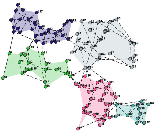
Figure 1.
An example of a partition over the IEEE 118 bus system using the modified k-means partitioning discussed in Case-III for five regions.
Figure 2a shows that non-homogeneous partitions will be formed by this strategy. However, because of the limitations of the local computing and communication capabilities (e.g., communication bandwidth, storage, and computational power), substantial inequalities in the sizes of the regions might not be appropriate. In order to overcome this issue, the aforementioned k-means method is modified to develop a size-constrained k-means algorithm that can produce homogeneous regions in terms of size. First, the grid will be divided into J non-homogeneous regions using the k-means algorithm, as mentioned above (assumed ). Then, the approximate ideal size of the homogeneous partitions is defined by the expression . In the following stage, the largest partition will be determined, and PMUs that are closest to the region’s center will be chosen and assigned to it. This area will be designated as finished and temporarily removed from the graph. For the reduced graph, the same procedure will be repeated. To be more precise, the assignments for the largest partition will be finalized when k-means is used to find non-homogeneous partitions on the reduced graph in the following step. Up till J homogeneous regions are obtained, this process will be repeated. If there are PMUs left out in the last step (due to ), they will be assigned to their closest region. An example distribution of homogeneous region sizes are presented in Figure 2b. This process is applied once before the state estimation and thus does not affect the computational complexity or run-time of the state estimation techniques.
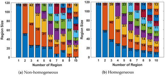
Figure 2.
Stacked representation of different region sizes for (a) non-homogeneous partitioning and (b) homogeneous partitioning discussed in Case-III. Each color represents a different region [3].
4.4. Case-IV: Multi-Area Distributed State Estimation with Information Sharing
In multi-area state estimation, allowing limited information sharing among the regions can improve the estimation accuracy by making the estimation process aware of the overall state of other regions and adaptive to changes in them. This case is an extension of Case-III, in which regions share selected data or features with their neighboring regions to be used in the local estimation process. In this work, various information-sharing schemes have been considered, as described next.
(a) Information Sharing through Overlapped Regions: In this scenario, common buses among regions are considered to enable information sharing among regions for the state estimation process. As such, instead of the partitioning mechanism presented in Case III, a soft clustering technique, specifically, fuzzy c-means (FCM) clustering [39,40], has been utilized to allow overlapping regions. The partitioning mechanism in this case is similar to the one presented in Case-III, except that buses can be assigned to multiple regions with varying degrees of membership belonging, where the membership can be tuned through specified thresholds. The process for keeping the region sizes homogeneous is the same as the hard partitioning mechanism presented in Case-III. An example of overlapped partition scenario has shown in Figure 3. The overlapping regions expand the feature space of individual regions by capturing partial information about the dynamics of neighboring regions through common buses.
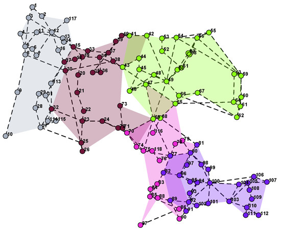
Figure 3.
An example of five overlapped regions discussed in Case-IV-a.
(b) Information Sharing through Auxiliary Buses: In this information-sharing technique, an auxiliary bus will be associated with each region, which is responsible to summarize and share the information about that region with the rest of the regions. As such, considering J regions, each region, say ith, will use data from its buses plus the data from auxiliary buses representing the rest of the regions.
The next step in information sharing through auxiliary buses is to assign features to them, such that the features embed the state information of the region that they are representing. The feature associated with the auxiliary bus of the region i at a specific time instance is denoted by . In this work, the following representing features are considered for :
- Mean of the state values of the buses of region i;
- State data of the bus with the largest variance in the region i;
- State data of the bus in the region i with maximum average correlation with the rest of the buses in the region i;
- State data of the bus in the region i with maximum average correlation with the buses in the region j;
- As the first principal component of states in region i.
5. Non-Linear Data-Driven Kalman Filter-based State Estimation
In addition to linear KF for modeling state estimation problem in power systems, non-linear KF has been considered to better track the non-linear dynamics of these systems. In the general non-linear system of equations, presented in Equation (1), functions and represent the non-linear measurement and system equations, respectively, which can be learned using data-driven techniques to track the system’s non-linear dynamics. To this end, the data-driven multivariate polynomial regression (MPR) model [41] has been utilized for non-linear system identification. Specifically, to have comparable linear and non-linear KF models, the non-linear auto-regressive exogenous model (NARX) has been considered in this paper as follows:
where is the total number of unique combinations of independent variables and p time-lagged measurements. If the order of the polynomial is considered to be , and represents the -th regressor.
5.1. Extended KF For Dynamic State Estimation
Extended KF (EKF) is a non-linear version of KF (here, named MPR-EKF), which specifies the non-linear systems and state equations at step k as:
Then, the main steps in EKF estimation are as follows:
(1) Prediction step:
(2) Correction step:
5.2. Unscented KF for Dynamic State Estimation
The propagation of error in covariance in Equation (21) through the linearization of the underlying non-linear model in EKF, as shown in Equation (19), can lead to poor performance in highly dynamic systems. In such circumstances, the unscented KF (UKF) can be applied, which generates a minimal set of sample points (known as sigma points) around the mean using the deterministic sampling technique known as the unscented transformation. The estimations of the new mean and error covariance are then generated from these altered sigma points using non-linear functions. The computation is performed in the following phases. First, sigma points are selected to propagate from k to time step using the best guess of and as follows, where is the diagonal element of matrix , and is an element of vector .
where represents the sigma point, i is the index of the sigma point, and N is the number of buses or states to be estimated. The variable denotes the change in sigma point, and both negative and positive changes are considered in defining sigma points. Next, the non-linear function is used to transform all the sigma points into as .
The initial state estimate will then be obtained by combining values as follows:
where is the modeling error and an element of . Using the updated estimate and , new sigma points will be computed as in Equation (25) to update the measurements . Then, the updated estimate can be calculated similarly to that of in Equation (26). The variance, (an element of ), and covariance, (an element of ), of the predicted measurements are calculated as follows:
where is the measurement error and an element of . The correction state can then be calculated as follows (denoted in vector and matrix notation):
One benefit of UKF over EKF is that it can reduce the computational complexity since it does not require calculating the Jacobin matrix in the estimation process. This approach is referred to as MPR-UKF in this paper.
6. Results
In this paper, the IEEE 118 bus system has been selected for the performance evaluation studies. First, a large dataset of PMU time-series are generated using the MATPOWER simulation toolbox [42], which we extended using real load profile data from the New York Independent System Operator (NYISO) dataset. Specifically, for each bus, voltage, phase angle, real power, and reactive power, , are recorded in the form of time-series. The cross-correlations of state variables among the buses have been calculated and used in the partitioning process (discussed in Case-III) to divide the system topology into multiple regions.
Following the discussion in Section 3, the state estimation problem has been considered for a range of scenarios from fully centralized to multi-area and fully distributed cases (labeled, Case-I to Case-IV). Moreover, various information-sharing mechanisms for collaborative state estimation among multi-areas (as discussed in Case-IV) have been considered for the performance evaluation studies. These scenarios have been considered for both linear and non-linear KF models. The results of the first study presented in Figure 4 show the estimation error for the two extreme cases where the state estimation is performed fully centralized or fully distributed. As expected, the estimation error is higher for the fully distributed estimation case (Case-I) both for linear and non-linear KF models, which is due to the limited information used for estimation at each individual bus. On the other hand, the fully centralized cases (Case-II) perform better due to the full observability and full-information access for all the buses. However, in the centralized cases, it is expected that the measurements from the geographically distributed components of the system are communicated to a central system for building models and developing functions such as state estimators. Communicating those measurements to a remote central system naturally imposes higher communication costs than localized models, which only use measurements from a local region in a distributed fashion. Studies have shown that lower dimensionality in the distributed estimation process results in a low communication cost [43]. In [9,44], it is also discussed that distributed state estimation enabled by new technologies, such as edge computing, can reduce the computational cost to lower than centralized processing of data. Moreover, it can be observed that non-linear KF models, particularly UKF, perform better estimation by better enabling the capture of non-linear dynamics of the system.
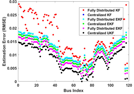
Figure 4.
The state estimation error at each bus for fully distributed and centralized estimation using MLR-KF, MPR-EKF, and MPR-UKF.
Next, the state estimation performance for a multi-area setting is considered both under a non-collaborative setting (Case-III) and various information-sharing mechanisms under Case-IV for the linear KF model. From Figure 5, it can be observed that as the number of regions increases, the performance of the state estimation decreases. Note that here the performance is calculated by taking the average estimation error over all the buses of the system. Moreover, it can be observed that allowing information sharing by overlapping a small subset of buses among the regions in Case-IV(a) results in better accuracy overall than in Case-III, which does not consider information sharing. Another approach to information sharing discussed in Case-IV(b) is to allow sharing a few resenting features from each region to help with state estimation. Among the various features discussed in Case-IV(b), sharing the state data of the bus in region i with a maximum average correlation with the buses in region j (named, Max Mutual Correlation case) results in better performance on average and particularly for the number of regions higher than four.
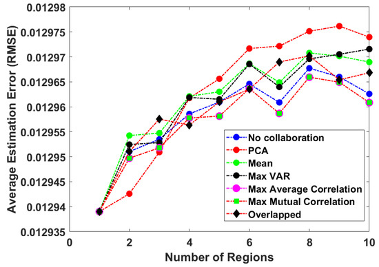
Figure 5.
Average estimation error over a varying number of regions for a different mode of information sharing among the regions for MLR-KF.
Figure 6 and Figure 7 also depict the performance of various modes of information sharing over multi-area distributed state estimation for EKF and UKF, respectively. A key observation here is that in the case of EKF and UKF with non-linear system approximations, the estimation error is decreasing with the increase in the number of regions. This can be explained through the characteristics of the average approximate entropy for different numbers of regions, as shown in Figure 8. Specifically, it has been discussed that entropy can be an indicator of the level of non-linearity in the system [45,46]. As can be observed from Figure 8, the average entropy over regions increases with the increase in the number of regions. Since a large number of regions is not generally practical for considering power systems, the trend observed for a small number of regions (up to ten) is considered in the studies in this paper. The result in Figure 8 suggests that as the number of regions increase, the non-linearity increases; as such, EKF and UKF performance show slight improvements compared to the opposite trend observed in Figure 5 for the linear KF model. Table 1 presents the average performance of various information-sharing approaches (i.e., average over various numbers of regions ranging from 1 to 10). From the table, it can be observed that maximum-mutual-correlation-based information-sharing approach results in the lowest estimation error for KF, EKF, and UKF. This result suggests that in the multi-area state estimation setting, sharing the state information of the bus with the maximum correlation with the buses of the other region can help improve the performance of the model while still only using local information.
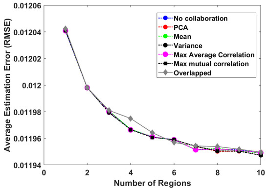
Figure 6.
Average estimation error over varying numbers of regions for different modes of information sharing among the regions for MPR-EKF.
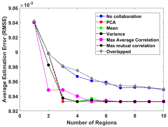
Figure 7.
Average estimation error over varying numbers of regions for different modes of information sharing among the regions for MPR-UKF.
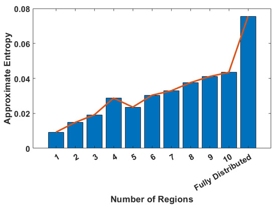
Figure 8.
Average approximate entropy as a measure of system non-linearity for different numbers of regions.

Table 1.
The average RMSE for state estimation using MLR-KF, MPR-EKF, and MPR-UKF for various information-sharing techniques.
While Table 1 shows the average performance with small differences, if Figure 5, Figure 6 and Figure 7 are considered, it can be observed that for different numbers of regions, the performance gains from different information-sharing approaches are different. Specifically, a comparatively wider range of variations in performance for different information-sharing approaches for different regions can be observed.
Next, the performances of the proposed techniques in this paper are compared with some of the existing methods in the literature, including historical averaging (HA) [47], support vector regression (SVR) [48], minimum mean square error (MMSE) state estimation method [5], Bayesian multivariate auto-regressive (BMLAR) [3], and temporal graph convolutional network (T-GCN) [4]. For comparison purposes, these techniques are applied to two scenarios, including centralized state estimation and multi-area state estimation with four regions. The number of regions are selected as four as it shows a good balance of state estimation performance based on the results presented in previous figures and also for practicality. Furthermore, no information sharing is considered in this comparison as the techniques from the literature are mainly developed for a centralized setting with no information-sharing mechanism in their original form. The average estimation error in the form of RMSE for Linear-KF, EKF, and UKF are presented in Table 2 as , , and , respectively, with UKF showing the leading performance. T-GCN shows a slightly better performance than MPR-UKF; it uses topological information (system’s adjacency matrix) as input. However, the availability of accurate topological information in certain cases cannot be considered. Additionally, the sensitivity to noise has been evaluated for 90 dB, 60 dB, and 30 dB of SNR, and the results in Table 3 show that linear-KF is more susceptible to noise compared to the non-linear KF models. However, the proposed methods retain acceptable performance up to 60 dB of SNR.
Table 2.
The average RMSE for various state estimation techniques for the centralized and multi-area state estimation with four regions and no information sharing.
Table 3.
The average RMSE for various noise levels for the proposed state estimation techniques with four regions and no information sharing.
7. Conclusions
In this work, a data-driven, multi-area distributed state estimation framework for smart grids have been discussed. Data-driven system identification techniques have been implemented to approximate the underlying power system dynamics in both linear and non-linear fashions. These data-driven system models are used to develop linear, extended, and unscented Kalman filter models for state estimation in the system. These data-driven models are particularly helpful in supporting state estimation under missing or limited measurements, such as in cases of partial unobservability due to failures or attacks in the sensing and monitoring system or limited availability of PMUs. The presented models are considered under various distributed settings, which can support low-latency requirements of critical functions and reduce the communication overhead through state estimation using local data from each region. Various modes of information sharing among the regions have also been studied to improve the performance of distributed state estimation. It has been shown through numerical evaluations that the distributed state estimation using data-driven linear and non-linear Kalman filters with selective feature sharing among the regions—particularly, sharing the state of a node with highest correlation with the other region—can lead to comparable results to centralized state estimation. The presented models also show a leading performance compared to some of the other data-driven and machine learning models in the literature.
Author Contributions
Conceptualization, M.J.H. and M.N.; Formal analysis, M.J.H.; Funding acquisition, M.N.; Supervision, M.N.; Writing—original draft, M.J.H.; Writing—review & editing, M.N. All authors have read and agreed to the published version of the manuscript.
Funding
This material is based upon work supported by the National Science Foundation under Grant No. 2118510.
Conflicts of Interest
The authors declare no conflict of interest.
References
- Weng, Y.; Negi, R.; Faloutsos, C.; Ilić, M.D. Robust Data-Driven State Estimation for Smart Grid. IEEE Trans. Smart Grid 2017, 8, 1956–1967. [Google Scholar] [CrossRef]
- Netto, M.; Mili, L. A Robust Data-Driven Koopman Kalman Filter for Power Systems Dynamic State Estimation. IEEE Trans. Power Syst. 2018, 33, 7228–7237. [Google Scholar] [CrossRef]
- Hossain, M.J.; Rahnamay-Naeini, M. Data-Driven, Multi-Region Distributed State Estimation for Smart Grids. In Proceedings of the 2021 IEEE PES Innovative Smart Grid Technologies Europe (ISGT Europe), Espoo, Finland, 18–21 October 2021; pp. 1–6. [Google Scholar]
- Hossain, M.J.; Rahnamay-Naeini, M. State Estimation in Smart Grids Using Temporal Graph Convolution Networks. In Proceedings of the 2021 North American Power Symposium (NAPS), College Station, TX, USA, 14–16 November 2021; pp. 1–5. [Google Scholar]
- Hossain, M.J.; Rahnamy-Naeini, M. Line Failure Detection from PMU Data after a Joint Cyber-Physical Attack. In Proceedings of the 2019 IEEE Power & Energy Society General Meeting (PESGM), Atlanta, GA, USA, 4–8 August 2019; pp. 1–5. [Google Scholar]
- Ji, X.; Yin, Z.; Zhang, Y.; Wang, M.; Zhang, X.; Zhang, C.; Wang, D. Real-time robust forecasting-aided state estimation of power system based on data-driven models. Int. J. Electr. Power Energy Syst. 2021, 125, 106412. [Google Scholar] [CrossRef]
- Tajer, A.; Kar, S.; Poor, H.V. Distributed state estimation: A learning-based framework. In Smart Grid Communications and Networking; Hossain, E., Han, Z., Poor, H.V., Eds.; Cambridge University Press: Cambridge, UK, 2012; pp. 191–202. [Google Scholar]
- Ma, H.; Yang, Y.H.; Chen, Y.; Liu, K.J.R. Distributed state estimation in smart grid with communication constraints. In Proceedings of the 2012 Asia Pacific Signal and Information Processing Association Annual Summit and Conference, Hollywood, CA, USA, 3–6 December 2012; pp. 1–4. [Google Scholar]
- Hasnat, M.A.; Hossain, M.J.; Adeniran, A.; Rahnamay-Naeini, M.; Khamfroush, H. Situational Awareness Using Edge-Computing Enabled Internet of Things for Smart Grids. In Proceedings of the 2019 IEEE Globecom Workshops (GC Wkshps), Waikoloa, HI, USA, 9–13 December 2019; pp. 1–6. [Google Scholar]
- Nakarmi, U.; Naeini, M.R.; Hossain, M.J.; Hasnat, M.A. Interaction Graphs for Cascading Failure Analysis in Power Grids: A Survey. Energies 2020, 13, 2219. [Google Scholar] [CrossRef]
- Wu, F.F. Power system state estimation: A survey. Int. J. Electr. Power Energy Syst. 1990, 12, 80–87. [Google Scholar] [CrossRef]
- Shivakumar, N.R.; Jain, A. A Review of Power System Dynamic State Estimation Techniques. In Proceedings of the 2008 Joint International Conference on Power System Technology and IEEE Power India Conference, New Delhi, India, 12–15 October 2008; pp. 1–6. [Google Scholar]
- Zhao, J.; Gómez-Expósito, A.; Netto, M.; Mili, L.; Abur, A.; Terzija, V.; Kamwa, I.; Pal, B.; Singh, A.K.; Qi, J.; et al. Power System Dynamic State Estimation: Motivations, Definitions, Methodologies, and Future Work. IEEE Trans. Power Syst. 2019, 34, 3188–3198. [Google Scholar] [CrossRef]
- Zhou, N.; Meng, D.; Huang, Z.; Welch, G. Dynamic State Estimation of a Synchronous Machine Using PMU Data: A Comparative Study. IEEE Trans. Smart Grid 2015, 6, 450–460. [Google Scholar] [CrossRef]
- Misyris, G.S.; Venzke, A.; Chatzivasileiadis, S. Physics-Informed Neural Networks for Power Systems. In Proceedings of the 2020 IEEE Power & Energy Society General Meeting (PESGM), Montreal, QC, Canada, 2–6 August 2020; pp. 1–5. [Google Scholar]
- Zhou, W.; Wu, Y.; Huang, X.; Lu, R.; Zhang, H.T. A group sparse Bayesian learning algorithm for harmonic state estimation in power systems. Appl. Energy 2022, 306, 118063. [Google Scholar]
- Bilil, H.; Gharavi, H. MMSE-Based Analytical Estimator for Uncertain Power System with Limited Number of Measurements. IEEE Trans. Power Syst. 2018, 33, 5236–5247. [Google Scholar]
- Zhang, J.; Welch, G.; Bishop, G.; Huang, Z. A Two-Stage Kalman Filter Approach for Robust and Real-Time Power System State Estimation. IEEE Trans. Sustain. Energy 2014, 5, 629–636. [Google Scholar] [CrossRef]
- Simon, D. Optimal State Estimation: Kalman, H Infinity, and Nonlinear Approaches; John Wiley & Sons: Hoboken, NJ, USA, 2006. [Google Scholar]
- Yang, Z.; Gao, R.; He, W. A Review of The Research on Kalman Filtering in Power System Dynamic State Estimation. In Proceedings of the 2021 IEEE 4th Advanced Information Management, Communicates, Electronic and Automation Control Conference (IMCEC), Chongqing, China, 18–20 June 2021; Volume 4, pp. 856–861. [Google Scholar]
- Soltan, S.; Mittal, P.; Poor, H.V. Line Failure Detection After a Cyber-Physical Attack on the Grid Using Bayesian Regression. IEEE Trans. Power Syst. 2019, 34, 3758–3768. [Google Scholar] [CrossRef]
- Liu, H.; Hu, F.; Su, J.; Wei, X.; Qin, R. Comparisons on Kalman-Filter-Based Dynamic State Estimation Algorithms of Power Systems. IEEE Access 2020, 8, 51035–51043. [Google Scholar] [CrossRef]
- Huang, Z.; Schneider, K.; Nieplocha, J. Feasibility studies of applying Kalman Filter techniques to power system dynamic state estimation. In Proceedings of the 2007 International Power Engineering Conference (IPEC 2007), Singapore, 3–6 December 2007; pp. 376–382. [Google Scholar]
- Khandelwal, A.; Tondan, A. Power system state estimation comparison of Kalman filters with a new approach. In Proceedings of the 2016 7th India International Conference on Power Electronics (IICPE), Patiala, India, 17–19 November 2016; pp. 1–6. [Google Scholar]
- Jin, X.B.; Robert Jeremiah, R.J.; Su, T.L.; Bai, Y.T.; Kong, J.L. The New Trend of State Estimation: From Model-Driven to Hybrid-Driven Methods. Sensors 2021, 21, 2085. [Google Scholar] [CrossRef]
- Kurt, M.N.; Yılmaz, Y.; Wang, X. Secure Distributed Dynamic State Estimation in Wide-Area Smart Grids. IEEE Trans. Inf. Forensics Secur. 2020, 15, 800–815. [Google Scholar] [CrossRef]
- Muscas, C.; Pau, M.; Pegoraro, P.A.; Sulis, S.; Ponci, F.; Monti, A. Multiarea Distribution System State Estimation. IEEE Trans. Instrum. Meas. 2015, 64, 1140–1148. [Google Scholar] [CrossRef]
- Korres, G.N. A Distributed Multiarea State Estimation. IEEE Trans. Power Syst. 2011, 26, 73–84. [Google Scholar] [CrossRef]
- Cosovic, M.; Tsitsimelis, A.; Vukobratovic, D.; Matamoros, J.; Anton-Haro, C. 5G Mobile Cellular Networks: Enabling Distributed State Estimation for Smart Grids. IEEE Commun. Mag. 2017, 55, 62–69. [Google Scholar] [CrossRef]
- Tran, M.Q.; Zamzam, A.S.; Nguyen, P.H.; Pemen, G. Multi-Area Distribution System State Estimation Using Decentralized Physics-Aware Neural Networks. Energies 2021, 14, 3025. [Google Scholar] [CrossRef]
- Sun, Y.; Zhao, Y. Distributed Cubature Kalman Filter with Performance Comparison for Large-scale Power Systems. Int. J. Control Autom. Syst. 2021, 19, 1319–1327. [Google Scholar] [CrossRef]
- Zegers, F.M.; Sun, R.; Chowdhary, G.; Dixon, W.E. Distributed State Estimation with Deep Neural Networks for Uncertain Nonlinear Systems under Event-Triggered Communication. arXiv 2022, arXiv:2202.01842. [Google Scholar]
- Vuković, O.; Dán, G. Security of Fully Distributed Power System State Estimation: Detection and Mitigation of Data Integrity Attacks. IEEE J. Sel. Areas Commun. 2014, 32, 1500–1508. [Google Scholar] [CrossRef]
- Zhang, X.; Shen, Y. Distributed Kalman Filtering Based on the Non-Repeated Diffusion Strategy. Sensors 2020, 20, 6923. [Google Scholar] [CrossRef]
- Jiang, Y.; Hui, Q. Kalman filter with diffusion strategies for detecting power grid false data injection attacks. In Proceedings of the 2017 IEEE International Conference on Electro Information Technology (EIT), Lincoln, NE, USA, 14–17 May 2017; pp. 254–259. [Google Scholar]
- Weng, S.; Yue, D.; Dou, C.; Shi, J.; Huang, C. Distributed Event-Triggered Cooperative Control for Frequency and Voltage Stability and Power Sharing in Isolated Inverter-Based Microgrid. IEEE Trans. Cybern. 2019, 49, 1427–1439. [Google Scholar] [CrossRef]
- Zhao, C.; Zhao, J.; Wu, C.; Wang, X.; Xue, F.; Lu, S. Power Grid Partitioning Based on Functional Community Structure. IEEE Access 2019, 7, 152624–152634. [Google Scholar] [CrossRef]
- Zhang, M.; Miao, Z.; Fan, L. Power Grid Partitioning: Static and Dynamic Approaches. In Proceedings of the 2018 North American Power Symposium (NAPS), Fargo, ND, USA, 9–11 September 2018; pp. 1–6. [Google Scholar]
- Bezdek, J.C. Pattern Recognition with Fuzzy Objective Function Algorithms; Springer Science + Business Media: New York, NY, USA, 1981. [Google Scholar]
- Mezquita, J.; Asber, D.; Lefebvre, S.; Saad, M.; Lagacé, P.J. Power network partitioning with a fuzzy C-means. In Proceedings of the IASTED International Conference on Power and Energy Systems and Applications (PESA 2011), Pittsburgh, PA, USA, 7–9 November 2011. [Google Scholar]
- Vaccari, D.A.; Wang, H.K. Multivariate polynomial regression for identification of chaotic time series. Math. Comput. Model. Dyn. Syst. 2007, 13, 395–412. [Google Scholar] [CrossRef]
- Zimmerman, R.D.; Murillo-Sánchez, C.E.; Thomas, R.J. MATPOWER: Steady-State Operations, Planning, and Analysis Tools for Power Systems Research and Education. IEEE Trans. Power Syst. 2011, 26, 12–19. [Google Scholar] [CrossRef]
- Garg, A.; Ma, T.; Nguyen, H. On communication cost of distributed statistical estimation and dimensionality. In Proceedings of the Advances in Neural Information Processing Systems, Montreal, QC, USA, 8–13 December 2014; Volume 27. [Google Scholar]
- Hudson, N.; Hossain, M.J.; Hosseinzadeh, M.; Khamfroush, H.; Rahnamay-Naeini, M.; Ghani, N. A Framework for Edge Intelligent Smart Distribution Grids via Federated Learning. In Proceedings of the 2021 International Conference on Computer Communications and Networks (ICCCN), Athens, Greece, 19–22 July 2021; pp. 1–9. [Google Scholar]
- Delgado-Bonal, A.; Marshak, A. Approximate Entropy and Sample Entropy: A Comprehensive Tutorial. Entropy 2019, 21, 541. [Google Scholar] [CrossRef]
- Pincus, S. Approximate entropy (ApEn) as a complexity measure. Chaos Interdiscip. J. Nonlinear Sci. 1995, 5, 110–117. [Google Scholar] [CrossRef]
- Weng, Y.; Negi, R.; Ilić, M.D. Historical data-driven state estimation for electric power systems. In Proceedings of the 2013 IEEE International Conference on Smart Grid Communications (SmartGridComm), Vancouver, BC, Canada, 21–24 October 2013; pp. 97–102. [Google Scholar]
- Kirinčić, V.; Čeperić, E.; Vlahinić, S.; Lerga, J. Support Vector Machine State Estimation. Appl. Artif. Intell. 2019, 33, 517–530. [Google Scholar] [CrossRef]
Publisher’s Note: MDPI stays neutral with regard to jurisdictional claims in published maps and institutional affiliations. |
© 2022 by the authors. Licensee MDPI, Basel, Switzerland. This article is an open access article distributed under the terms and conditions of the Creative Commons Attribution (CC BY) license (https://creativecommons.org/licenses/by/4.0/).