Article

How to Train an Artificial Neural Network to Predict Higher Heating Values of Biofuel

1
Institute of Solid State Chemistry and Mechanochemistry, 18 Kutateladze Str., 630090 Novosibirsk, Russia
2
Department of Business, Novosibirsk State Technical University, 20 Karl Marx Ave., 630073 Novosibirsk, Russia
*
Author to whom correspondence should be addressed.
Energies 2022, 15(19), 7083; https://doi.org/10.3390/en15197083
Submission received: 20 August 2022 / Revised: 20 September 2022 / Accepted: 23 September 2022 / Published: 27 September 2022

Abstract

:
Plant biomass is one of the most promising and easy-to-use sources of renewable energy. Direct determination of higher heating values of fuel in an adiabatic calorimeter is too expensive and time-consuming to be used as a routine analysis. Indirect calculation of higher heating values using the data from the ultimate and proximate analyses is a more rapid and less equipment-intensive method. This study assessed the fitting performance of a multilayer perceptron as an artificial neural network for estimating higher heating values of biomass. The analysis was conducted using a specially gathered large and heterogeneous dataset (720 biomass samples) that included the experimental data of ultimate and proximate analysis on grass plants, peat, husks and shells, organic residues, municipal solid wastes, sludge, straw, and untreated wood. The quantity and preprocessing of data (namely, rejection of dependent and noisy variables; dataset centralization) were shown to make a major contribution to prediction accuracy improvement. In particular, it was demonstrated that 550 samples are sufficient to ensure convergence of the algorithm; carbon and hydrogen contents are sufficient ultimate analysis data; and volatile matters can be excluded from proximate analysis. The minimal required complexity of neural network is ~50 neurons.

1. Introduction

Studies addressing energy production from plant biomass are still relevant today [1,2,3]. The optimal sources of plant biomass suitable for biofuel production are selected and the processes of treatment and combustion of biomass fuel, both individually and in blends with coal of different grades, are optimized in these works [4,5,6]. In this connection, the analysis methods making it possible to determine the thermophysical properties of the feedstock and fuel obtained from it are being mastered. Fuel combustion in an adiabatic calorimeter is the most accurate method for determining the heating values of solid fuels. However, procedures for predicting higher heating values (HHVs) based on the data from proximate and ultimate analyses are currently being developed for the cases when the aforementioned method is infeasible. More than 150 empirical correlation equations [6,7,8,9,10,11] for calculating the heating values of various lignocellulosic feedstocks are known today. The correlations obtained for one type of biomass, however, may fail to provide accurate results when the heating value is calculated for a different type of biomass. There are very few universal equations, and finding these equations and refining their coefficients is a rather labor-intensive task [11,12].
Due to the advances in mathematical methods, the past years have witnessed an upsurge of interest in using self-training artificial neural networks (ANNs) to handle large datasets. When a representative initial data set (the training set) is available for a researcher, the artificial neural network can reveal an implicit dependence that can yield an appreciably accurate result for other input data (the test set) [13]. Studies showing the potential of the artificial neural network model in predicting the heating values based on the data from proximal and ultimate analysis have been published [14,15,16,17]. They compared the results of predictions made using the conventional correlation equations and neural networks, and analyzed the efficiency of logistics, combustion, pyrolysis, and torrefaction of coal/biomass blends [18,19,20].
Unfortunately, it must be admitted that some of the available publications do not take into account such important methodological aspects as the size and homogeneity of the training set. It occurs quite often that the size of the initial data set used for training the artificial neural network is rather small (~100, very rarely over 200–300), and there are only minor differences between these data [21,22,23,24]. When this approach is used, the algorithm yields expectedly good results, but the same problem as the one related to the empirical models emerges: the applicability of the algorithm trained using a homogeneous and narrowly specialized set for predicting the heating values of other biomass types (e.g., the biomass with higher lignin or ash contents).
Furthermore, it is known that aside from training, the neural network also requires hyperparameter tuning (i.e., optimization of the set of parameters determining its operation algorithm). This means that a single training cycle is not sufficient: many iterations need to be performed, the results of training for the testing set need to be compared each time, and hyperparameters need to be varied. No clear algorithm for such iterative tuning exists today. Researchers make their own decisions on which hyperparameters should be changed and in which order it needs to be done to yield the optimal results through trial and error. Unlike in the pioneer studies focusing on this topic [25], the authors of papers on the practical use of ANNs [26] often report neither the resulting optimal values of hyperparameters nor the network trained using the optimal hyperparameters, so their results cannot be reproduced.
This article attempts to solve both these problems. Indeed, since there are quite a few publications on using ANNs to predict HHVs based on the data from ultimate or proximate analysis, we place special emphasis on the fact that ANN is a complex tool requiring pre-tuning rather than simply stating that the ANN can be efficient for solving the problem. Furthermore, it was important to demonstrate the significant role played by the quantity of input data in prediction accuracy. In other words, this study aimed to demonstrate the process of tuning the artificial neural network to predict higher heating values of biomass when analyzing a large and extremely heterogeneous dataset, as well as to compare the results obtained using an ANN with those obtained using the universal empirical formulas.

2. Materials and Methods

2.1. Data Collection

A dataset collected from the open Phyllis2 database (the database containing information on compositions of biomass, macro- and microalgae, feedstocks for biogas production, biochar and torrefied biomass) [27], published reviews [7,28,29], and authors’ own data obtained earlier [12] were used in this study.
When collecting the data, it was taken into account that each individual sample (type of biomass) needs to be simultaneously described using the following parameters: the measured higher heating value, and the data from ultimate analysis (carbon, hydrogen, and nitrogen contents) and proximate analysis (ash content, volatile matter, and fixed carbon). All the data were provided on a dry matter basis. The proximate analysis was confined to carbon, hydrogen, and nitrogen contents, so such elements as oxygen, sulfur, chlorine, and phosphorus could be omitted from consideration, as it is difficult to accurately measure their contents in the routine mode.
An important feature of the ANN is its generalization ability (i.e., its ability to adequately respond to the outliers in the training data). In this connection, the collected data were not subjected to any statistical processing aimed at making the dataset more homogeneous or narrow.
For illustrative purposes, all the samples were categorized into groups according to the classification used in the Phyllis2 database (Table 1). The full dataset is provided in the Supplementary File “Initial Dataset.xls”.

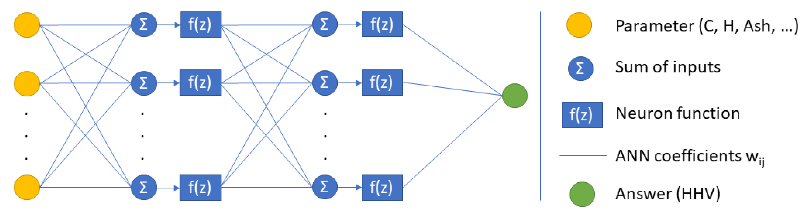
2.2. Artificial Neural Network Architecture and Evaluation

A software environment where both dataset parameters and hyperparameters of the ANN can be appreciably easily set and varied is needed to work with an ANN. Many existing studies predicting the HHVs of the biomass were performed using the MatLab and Python environments [14,16,17,24]. The Python environment stands out, as it is affordable, popular, and easy to use (also being friendly for novice users). Thus, the scikit-learn library contains the algorithm of a full-connected perceptron MLP Regressor implemented as a function with a set of user-defined hyperparameters, which is used in most studies, and integrated algorithms for data preprocessing.
Figure 1 shows the general schematic diagram for MLP-ANN. The ANN with an arbitrary number of parameters of the input data, two hidden layers (each layer having an arbitrary number of neurons), and a single output value is shown here. Each neuron is shown as two components: the first component sums up all the inputs, while the second one calculates the response function from this sum and sends the new value to all the neurons at the next layer. The relationships between the ith and the jth elements imply that the transmitted value is multiplied by the coefficient wij, which is individual for each relationship. ANN variants having several (1 to 6) hidden layers, as well as a varied set of input parameters and neural response function, will be used further in this study.

3. Results and Discussion

3.1. Scoring and Rules

Before discussing neural network tuning, one should choose the outcome assessment criterion. There may be some particular cases where a criterion selected by a certain user of the ANN is important for him/her (e.g., it is extremely undesirable that the predicted HHV is higher than the true one, while underestimation is permissible and less critical.) The mean absolute error (MAE) and mean squared error (MSE) of the prediction are used most commonly nowadays. MAE is less sensitive to the large number of outliers in the dataset than MSE. However, according to the Cramér’s theorem, MSE is the optimal validation criterion between the data and the model for a random error in Gaussian distribution [30]. Since the absolute MSE value is linked to the preprocessing method, the normalized MSE (R2 criterion, or the “proportion of explained set”) is used frequently (1):
R 2 = 1 y i y p r e d   i 2 y i y m e a n 2 ,
where y i is the true HHV of the ith sample; y p r e d   i is the neural network prediction for the same sample;   y m e a n is the mean HHV in the entire dataset. In this study, we use the MSE criterion as a built-in method for error estimation during neural network training, as well as the R2 criterion for iterative tuning of hyperparameters.
The key logical components of an artificial neural network, according to the order of their effect on the output provided by the algorithm, as follows:
1.
Training set;
2.
The ANN architecture (the number of neurons and the number of layers);
3.
Neural response function;
4.
The solver algorithm.
Since the ANN searches for hidden regularities in inputs instead of providing additional information, its output primarily depends on the inputs. Next, the feasibility of searching for hidden regularities is determined by the complexity of the neural network, so the ANN architecture was ranked second. The third component is neural response function, which determines the functional properties of ANN and training-related components. Indeed, if the more important components are properly implemented, all that is left to do is properly train the neural network.
It is safe to say that all the components listed above except the first one are mathematically independent. This assumption and the corresponding arranging of ANN components according to their importance makes it possible to propose the following tuning algorithm. First, some initial values for all hyperparameters are set, and the optimal value for the most important hyperparameter is then found. In the following step, the next hyperparameter is varied and optimized, and so on. Let us discuss each tuning step in the suggested order of ANN components.

3.2. Preprocessing of the Inputs for Predicting the HHVs

As already mentioned, the ANN outputs primarily depend on inputs. Therefore, the user’s main concern is to prepare these data to ensure proper performance of the neural network.
Parameters (features) of inputs correlated most strongly with the target parameter HHV identified at the first step. In our case, each sample is characterized by six parameters: three ultimate analysis parameters (carbon, hydrogen, and nitrogen contents) and three proximate analysis parameters (ash content, volatile matter, and fixed carbon).
Pearson’s correlation coefficients (Table 2) show that nitrogen content is weakly correlated with HHV, probably due to the high error of determining nitrogen content. In the ideal case, ANN is supposed to filter the noisy data, but it is quite possible that prediction accuracy will be worsened because of the input noise caused by other “negative factors” (e.g., significant sample heterogeneity or experimental errors).
Furthermore, it is clear that parameters determined by proximate analysis are not independent. Thus, the volatile matter was calculated arithmetically by subtracting the weights of ash and fixed carbon from the initial sample weight. Using all three proximate analysis parameters for ANN training artificially overestimates their weights, so it would be more correct to use only two of them for calculations.
Let us consider the results of comparing the following data:
-
The individual data from ultimate analysis (Set 1);
-
The individual data from proximate analysis (Set 2);
-
A combination of the data from ultimate and proximate analyses (Set 3);
-
A combination of the data from ultimate and proximate analyses, except for nitrogen content and volatile matter (Set 4).
According to standard practice, each dataset is divided into the training and test sets at a 3:1 ratio; i.e., the training set contains 540 samples, while the test set contains 180 samples. Randomization is mandatorily performed prior to this division (Figure 2).
The next step of data preprocessing involved normalization (2) and centralization (3) of the input dataset. Both procedures ensure the heterogeneity of input parameters, so the ANN takes them into account to an equal extent.
X s c a l e d = x x . m i n x . m a x x . m i n m i n m a x + m a x ,
where x.max and x.min are the maximal and minimal values of the input parameter x before scaling, respectively; max and min are the user-defined maximal and minimal Xscaled values after scaling, respectively (we used max = 1 and min = −1).
X s c a l e d = x x . m e a n x . s t d ,
where x.mean is the mean value in the sample and x.std is the standard deviation of the mean value in the sample.
Figure 3 and Figure 4 and Table 3 show the results of comparing the efficiencies of ANN performance for the four variants of inputs and two variants of their preprocessing.
One can see that dataset normalization is more likely to worsen the prediction accuracy of ANN, while centralization consistently improves it. Moreover, normalization and centralization have different effects on the convergence rate: whereas algorithm convergence for the initial dataset requires up to 460 iterations, the normalized and centralized datasets require 40 and 100–240 iterations to converge, respectively.
As expected, prediction of HHV based on the data from proximate analysis (Set 2) was inaccurate for the initial dataset being so heterogeneous in terms of the analyzed objects. However, prediction accuracy was significantly improved by using its combination with the data from ultimate analysis (Set 3). Furthermore, the results proved the assumption that rejecting noisy and dependent variables from consideration will improve the prediction accuracy. The best results were obtained for the dataset (Set 4) where the data on nitrogen content and volatile matter were rejected. In this connection, the data from this dataset (Set 4) will be used for further work.

3.3. ANN Architecture Tuning

The ANN architecture needs to be well balanced; it should be appreciably complex to be able to detect hidden regularities, but not too intricate so that overfitting is avoided. The fully connected multilayer perceptron used in this study allows one to vary the number of layers and the number of neurons per layer.
The architecture was gradually made more intricate. First, the number of neurons for a single-layer ANN was varied. This procedure was then repeated for the ANN having a larger number of layers. The occurrence of overfitting was the key optimization criterion. It is generally believed that a sign of overfitting is that the neural system starts providing inaccurate predictions for the test set. This was not observed in our case, so another sign of overfitting occurrence was used (the instant when prediction using the training set is much more accurate than the prediction provided by the same neural network for the test set). Figure 5 shows the diagrams for the prediction error as a function of the number of neurons per layer for the ANN with 1–6 hidden layers.
One can see that overfitting occurs earlier as the number of layers increases. It is interesting to note that the single-layer perceptron (1D ANN) differs from the multilayer ones in terms of the optimal number of neurons. This number is 250 for the 1D ANN and approximately 40–50 for the multilayer ones. It can easily be checked that distribution of neurons over layers is not important for the multilayer perceptron. An attempt to redistribute 50 neurons between the two layers demonstrated that except for the extreme cases (up to 5 neurons in one layer and 45 neurons in the other layer), neural configuration in the layers does not significantly affect prediction accuracy (Figure 6a). Convergence is attained in 300 iterations, regardless of the architecture (Figure 6b).
The final decision regarding the single-layer ANN architecture was made on the basis of Figure 6c. Indeed, the two-layer ANN architecture (25 and 25 neurons per layer), although being optimal in terms of overfitting, does not provide prediction accuracy higher than 0.9. The 2D-ANN reaches R2 > 0.9 only after overfitting. For the 1D-ANN architecture, R2 > 0.9 is reached already when there are 50 neurons per layer, while its overfitting occurs when the neuron number is 250. The 3D-ANN provides an overly significant dispersion of R2.

3.4. Choosing the Activation Function

Activation functions determining the response of individual neurons depending on the magnitude of input values play a crucial role in ANN tuning. The most commonly used functions are as follows: (4) no-op activation (useful to implement linear bottleneck), (5) logistic sigmoid, (6) hyperbolic, and (7) rectified linear unit function.
f(x) = x
f(x) = 1/(1 + exp(−x))
f(x) = tanh(x)
f(x) = max(0, x)
Table 4 lists the results of testing the selected activation functions for the analyzed dataset. The rectified linear unit function yields the best result; in combination with the good results of using the no-op activation function, this demonstrates that HVV prediction is a nearly regression problem [31].

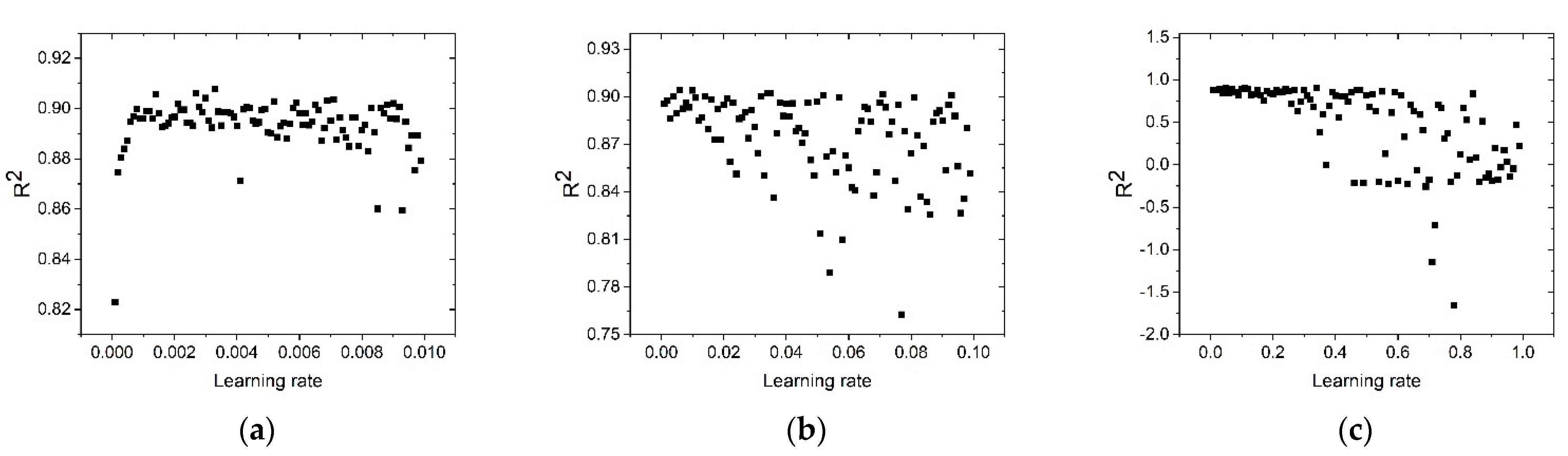
3.5. Optimizing the Operation of the Solver Algorithm

Neural networks are trained using the error back-propagation algorithm. Random state sets the values to arbitrary initial coefficients before the operation; the prediction error σ 0 (the difference between the value predicted by ANN and the true value of the target parameter) is then calculated for each sample of the training set (in our case, it is the HHV value). Next, the prediction error is calculated for each successive neuron; summing up is performed for the neurons of the previous layer (error backpropagation takes place).
σ j = w k j o l d σ k ,     w h e r e   σ 0 = y y p r e d
The initial coefficient values are then varied according to the selected rule. In the stochastic gradient descent without regularization, this rule is formulated as follows:
w i j n e w = w i j o l d + λ × σ j × d f z d z z j o l d
where f(z) is the neural network activation function; λ is the learning rate; z j o l d is the value at the input of the jth neuron at the previous training step.
Today, the conventional gradient descent method is almost never used in its non-modified form. Its numerous modifications aim to eliminate the major drawbacks of the method. For example, the stochasticity of training is eliminated by using mini batches: in this variant, the coefficients are adjusted after analyzing a small batch of samples rather than each individual sample. The size of this batch depends on the batch size parameter. Still, the coefficients can be too large or too small at a certain training stage (the so-called “neural burnout”). This phenomenon is eliminated by using regularization, when the attempts to change the previous coefficient values are smoothened with a certain efficiency α.
Deeper modifications to the conventional algorithm of stochastic gradient descent “sgd” are implemented in the analyzed MLP Regressor as two separate variants of solver algorithms: “adam” and “lbfgs”. Each of these is characterized by its own specific adjustments and scope of application. The most commonly used solver “adam” works fairly well on relatively large datasets (with thousands of training samples or more) in terms of both training time and validation score. For small datasets, however, “lbfgs” can converge faster and perform better. Indeed, the next R2 values are obtained for all solvers and then an Adaptive Moment Estimation is selected (Table 5).
Figure 7 and Figure 8 show the regularization procedure. Figure 8a shows that in our case, regularization reduces the stochasticity: the smaller the regularization parameter (α), the smaller the dispersion of R2 values depending on this parameter. The value α = 0.0001 was used by default, but we used α = 0.00001 for further calculations based on Figure 8a.
Figure 8b shows the results of tuning the mini batch size. One can see that it is actually more efficient to use mini batches rather than individual samples for training the algorithm. Mini batches containing 150–400 samples can be used to ensure stable performance of the algorithm. It seems that when analyzing such a dataset with heterogeneous absolute parameters, the ANN needs to analyze most of the dataset (or the entire dataset if it is appreciably small) in order to properly assess the problem. With allowance for the aforementioned arguments, a batch size value of 200 was used for further work.
The adam algorithm was not tuned with respect to specific parameters; however, it is worth mentioning that this tuning negligibly improves the R2 value. The full set of tuning parameters is presented in the Supplementary File“CHN-for-paper”. Sample size was the most critical parameter for the problem being discussed: only the datasets containing more than 550 samples ensure stable performance of the algorithm (Figure 8c). This result agrees with the simple rules of thumb. One rule of thumb is that the sample size needs to be 50 to 1000 times larger than the number of prediction classes (which, in the choice modelling context, is the choice set size) [32,33]. Another rule of thumb is that the sample size needs to be 10 to 100 times larger than the number of the features (which, in the choice modelling context, is the number of attributes) [34,35,36].
The applied approach to tuning ANN hyperparameters, which took into account the a priori considerations about neural network performance, significantly accelerates tuning compared to the conventional non–a priori searching approaches. Indeed, there are two simple approaches to searching for the optimal set of hyperparameters: the search with a specified increment over the entire hyperspace (GridSearchCV) or the search across the set number of arbitrary combinations of hyperparameters (RandomizedSearchCV). Both these examples have a computational complexity proportional to P m , where P is the number of hyperparameters and m is the number of permissible values for each of them. The approach proposed is characterized by a computational complexity of ~ P × m ; furthermore, it is sufficiently intuitive for the user.

3.6. Comparing the Prediction Accuracies Ensured Using ANN and the Empirical Formulas

In order to compare the accuracy of predictions made using the MLP Regressor and the existing empirical models, Equations (10) and (11) from [12] were used, since the greatest applicability for separate samples has been demonstrated for these equations:
Q = 0.4373⋅C − 1.6701
Q = 0.00355⋅C2 − 0.232⋅C − 2.230⋅H + 0.0512⋅C⋅H + 0.131⋅N + 20.600
Two alternative approaches were employed to evaluate the final performance of ANN. Both these approaches are used to eliminate the effect of ANN re-adaptation to a specific test sample. One of them, k-fold cross-validation, involves determining the scoring criteria for several variants of subdivision of the original dataset into the training and test sets. The benefit of this method is that it allows one to determine not only the average generalization performance but also the prediction model stability [37,38,39]. For our problem, this approach yields R2 = 0.880 ± 0.025. An alternative method is calculating the ANN prediction for the entire dataset being used. For our problem, this method yields R2 = 0.884. In other words, both these approaches yield identical (within the error) estimations of the final performance of ANN. The advantage of the second approach is that it allows one to easily and rather promptly compare the ANN predictions to those obtained using empirical formulas. Indeed, one can see in Figure 9 that the ANN has a much better prediction ability.

4. Conclusions

Hence, the fully connected perceptron used for the analyzed set characterized by very significant heterogeneity but an appreciably large size allows one to reach R2 = 0.880 ± 0.025. Our final suggestion for the ANN structure is as follows: perceptron with 100 neurons at hidden layer, rectangular unit function (relu) as activation function, and adaptive moment estimation (adam) as the training algorithm. (The full set of tuning parameters is presented in the Supplementary)
It turned out for our problem that data quantity and data preprocessing (namely, rejection of dependent variables and noisy values, as well as sample centralizing) make a major contribution to prediction accuracy improvement. The proposed tuning algorithm allows one to reduce time expenditure: from the power-law dependence of the number of permissible values of each hyperparameter to a dependence that is a result of multiplication by this value.
As with other ANNs, our ANN guarantees work only within the range where it was trained. However, it is a very wide range; it is the widest among other ranges reported previously. We consider ANN rather than any other machine learning approach because we would like to change the focus of discussion from small datasets and hidden hyperparameter optimization to step-by-step demonstration of hyperparameter tuning. ANN is convenient for such consideration. Other machine learning approaches were excluded due to reasonable restrictions on the scope of the article.

Supplementary Materials

The following supporting information can be downloaded at: https://www.mdpi.com/article/10.3390/en15197083/s1.

Author Contributions

Conceptualization, A.B.; methodology, A.B. and A.M.; validation, A.M.; formal analysis, A.M.; resources, A.B.; data curation, A.B. and A.M.; writing—original draft preparation, A.B. and A.M.; writing—review and editing, A.B.; visualization, A.M.; supervision, A.B. All authors have read and agreed to the published version of the manuscript.

Funding

The collection of raw data was supported by the Russian Science Foundation (project No. 21-13-00046). The mathematical analysis was supported by the state assignment to the Institute of Solid State Chemistry and Mechanochemistry SB RAS (No. FWUS-2021-0005).

Data Availability Statement

Not applicable.

Acknowledgments

The authors thank Anastasia Krokhina, a student at Novosibirsk State University, for her help in processing the primary data.

Conflicts of Interest

The authors declare no conflict of interest.

References

  1. Dafnomilis, I.; Hoefnagels, R.; Pratama, Y.W.; Schott, D.L.; Lodewijks, G.; Junginger, M. Review of solid and liquid biofuel demand and supply in Northwest Europe towards 2030—A comparison of national and regional projections. Renew. Sustain. Energy Rev. 2017, 78, 31–45. [Google Scholar] [CrossRef]
  2. Mandley, S.; Daioglou, V.; Junginger, H.; van Vuuren, D.; Wicke, B. EU bioenergy development to 2050. Renew. Sustain. Energy Rev. 2020, 127, 109858. [Google Scholar] [CrossRef]
  3. Titova, E.S. Biofuel Application as a Factor of Sustainable Development Ensuring: The Case of Russia. Energies 2019, 12, 3948. [Google Scholar] [CrossRef]
  4. Proskurina, S.; Junginger, M.; Heinimö, J.; Tekinel, B.; Vakkilainen, E. Global biomass trade for energy—Part 2: Production and trade streams of wood pellets, liquid biofuels, charcoal, industrial roundwood and emerging energy biomass. Biofuels Bioprod. Biorefining 2019, 13, 371–387. [Google Scholar] [CrossRef]
  5. Pradhan, P.; Mahajani, S.M.; Arora, A. Production and utilization of fuel pellets from biomass: A review. Fuel Process. Technol. 2018, 181, 215–232. [Google Scholar] [CrossRef]
  6. Kim, J.-H.; Jung, S.; Lin, K.-Y.A.; Rinklebe, J.; Kwon, E.E. Comparative study on carbon dioxide-cofed catalytic pyrolysis of grass and woody biomass. Bioresour. Technol. 2021, 323, 124633. [Google Scholar] [CrossRef]
  7. Yin, C.Y. Prediction of higher heating values of biomass from proximate and ultimate analyses. Fuel 2011, 90, 1128–1132. [Google Scholar] [CrossRef]
  8. Vargas-Moreno, J.; Callejón-Ferre, A.; Pérez-Alonso, J.; Velázquez-Martí, B. A review of the mathematical models for predicting the heating value of biomass. Renew. Sustain. Energy Rev. 2012, 16, 3065–3083. [Google Scholar] [CrossRef]
  9. Qian, C.; Li, Q.; Zhang, Z.; Wang, X.; Hu, J.; Cao, W. Prediction of higher heating values of biochar from proximate and ultimate analysis. Fuel 2020, 265, 116925. [Google Scholar] [CrossRef]
  10. Górnicki, K.; Kaleta, A.; Winiczenko, R. Prediction of higher heating value of oat grain and straw biomass. E3S Web Conf. 2020, 154, 01003. [Google Scholar] [CrossRef] [Green Version]
  11. Maksimuk, Y.; Antonava, Z.; Krouk, V.; Korsakova, A.; Kursevich, V. Prediction of higher heating value based on elemental composition for lignin and other fuels. Fuel 2019, 263, 116727. [Google Scholar] [CrossRef]
  12. Bychkov, A.L.; Denkin, A.I.; Tikhova, V.; Lomovsky, O. Prediction of higher heating values of plant biomass from ultimate analysis data. J. Therm. Anal. Calorim. 2017, 130, 1399–1405. [Google Scholar] [CrossRef]
  13. Cybenko, G. Approximation by superpositions of a sigmoidal function. Math. Control. Signals Syst. 1989, 2, 303–314. [Google Scholar] [CrossRef]
  14. Xing, J.; Luo, K.; Wang, H.; Gao, Z.; Fan, J. A comprehensive study on estimating higher heating value of biomass from proximate and ultimate analysis with machine learning approaches. Energy 2019, 188, 116077. [Google Scholar] [CrossRef]
  15. Obafemi, O.; Stephen, A.; Ajayi, O.; Nkosinathi, M. A survey of artificial neural network-based prediction models for thermal properties of biomass. Procedia Manuf. 2019, 33, 184–191. [Google Scholar] [CrossRef]
  16. Estiati, I.; Freire, F.B.; Freire, J.T.; Aguado, R.; Olazar, M. Fitting performance of artificial neural networks and empirical correlations to estimate higher heating values of biomass. Fuel 2016, 180, 377–383. [Google Scholar] [CrossRef]
  17. Uzun, H.; Yıldız, Z.; Goldfarb, J.L.; Ceylan, S. Improved prediction of higher heating value of biomass using an artificial neural network model based on proximate analysis. Bioresour. Technol. 2017, 234, 122–130. [Google Scholar] [CrossRef]
  18. Cao, H.; Xin, Y.; Yuan, Q. Prediction of biochar yield from cattle manure pyrolysis via least squares support vector machine intelligent approach. Bioresour. Technol. 2016, 202, 158–164. [Google Scholar] [CrossRef]
  19. Ozonoh, M.; Oboirien, B.O.; Daramola, M.O. Optimization of process variables during torrefaction of coal/biomass/waste tyre blends: Application of artificial neural network & response surface methodology. Biomass Bioenergy 2020, 143, 105808. [Google Scholar] [CrossRef]
  20. Goettsch, D.; Castillo-Villar, K.K.; Aranguren, M. Machine-learning methods to select potential depot locations for the supply chain of biomass co-firing. Energies 2020, 13, 6554. [Google Scholar] [CrossRef]
  21. Li, H.; Xu, Q.; Xiao, K. Predicting the higher heating value of syngas pyrolyzed from sewage sludge using an artificial neural network. Environ. Sci. Pollut. Res. 2020, 27, 785–797. [Google Scholar] [CrossRef] [PubMed]
  22. Olatunji, O.O.; Akinlabi, S.; Madushele, N.; Adedeji, P.A.; Felix, I. Multilayer perceptron artificial neural network for the prediction of heating value of municipal solid waste. AIMS Energy 2019, 7, 944–956. [Google Scholar] [CrossRef]
  23. Dashti, A.; Noushabadi, A.S.; Raji, M.; Razmi, A.; Ceylan, S.; Mohammadi, A.H. Estimation of biomass higher heating value (HHV) based on the proximate analysis: Smart modeling and correlation. Fuel 2019, 257, 115931. [Google Scholar] [CrossRef]
  24. Elmaz, F.; Büyükçakır, B.; Yücel, Ö.; Mutlu, A.Y. Classification of solid fuels with machine learning. Fuel 2020, 266, 117066. [Google Scholar] [CrossRef]
  25. Akkaya, E.; Demir, A. Predicting the heating value of municipal solid waste-based materials: An artificial neural network model. Energy Sources Part A Recover. Util. Environ. Eff. 2010, 32, 1777–1783. [Google Scholar] [CrossRef]
  26. Abidoye, L.K.; Mahdi, F.M. Novel linear and nonlinear equations for the higher heating values of municipal solid wastes and the implications of carbon to energy ratios. J. Energy Technol. Policy 2014, 4, 14–27. [Google Scholar]
  27. Phyllis2, Database for (Treated) Biomass, Algae, Feedstocks for Biogas Production and Biochar. TNO Biobased and Circular Technologies. Available online: https://phyllis.nl (accessed on 20 July 2022).
  28. Parikh, J.; Channiwala, S.A.; Ghosal, G.K. A correlation for calculating HHV from proximate analysis of solid fuels. Fuel 2005, 84, 487–494. [Google Scholar] [CrossRef]
  29. Krishnan, R.; Hauchhum, L.; Gupta, R.; Pattanayak, S. Prediction of equations for higher heating values of biomass using proximate and ultimate analysis. In Proceedings of the 2nd International Conference on Power, Energy and Environment: Towards Smart Technology (ICEPE), Shillong, India, 1–2 June 2018. [Google Scholar] [CrossRef]
  30. Myung, I.J. Tutorial on Maximum Likelihood Estimation. J. Math. Psychol. 2003, 47, 90–100. [Google Scholar] [CrossRef]
  31. Holzmüller, D.; Steinwart, I. Training two-layer ReLU networks with gradient descent is inconsistent. arXiv 2020, arXiv:2002.04861. [Google Scholar] [CrossRef]
  32. Cho, J.; Lee, K.; Shin, E.; Choy, G.; Do, S. How much data is needed to train a medical image deep learning system to achieve necessary high accuracy? arXiv 2015, arXiv:1511.06348. Available online: https://arxiv.org/pdf/1511.06348.pdf (accessed on 20 July 2022).
  33. Cireşan, D.C.; Meier, U.; Schmidhuber, J. Transfer learning for Latin and Chinese characters with deep neural networks. In Proceedings of the 2012 International Joint Conference on Neural Networks (IJCNN), Brisbane, Australia, 10–15 June 2012. [Google Scholar] [CrossRef] [Green Version]
  34. Jain, A.K.; Chandrasekaran, B. 39 Dimensionality and sample size considerations in pattern recognition practice. In Handbook of Statistics; Elsevier: Amsterdam, The Netherlands, 2001; Volume 2, pp. 835–855. [Google Scholar] [CrossRef]
  35. Kavzoglu, T.; Mather, P.M. The use of backpropagating artificial neural networks in land cover classification. Int. J. Remote Sens. 2003, 24, 4907–4938. [Google Scholar] [CrossRef]
  36. Raudys, S.J.; Jain, A.K. Small sample size effects in statistical pattern recognition: Recommendations for practitioners. IEEE Trans. Pattern Anal. Mach. Intell. 1991, 13, 252–264. [Google Scholar] [CrossRef]
  37. Kohavi, R. A study of cross-validation and bootstrap for accuracy estimation and model selection. In Proceedings of the 14th International Joint Conference on Artificial Intelligence, Montreal, QC, Canada, 20–25 August 1995. [Google Scholar]
  38. Rodriguez, J.D.; Perez, A.; Lozano, J.A. Sensitivity analysis of k-fold cross validation in prediction error estimation. IEEE Trans. Pattern Anal. Mach. Intell. 2009, 32, 569–575. [Google Scholar] [CrossRef]
  39. Bengio, Y.; Grandvalet, Y. No unbiased estimator of the variance of k-fold cross-validation. J. Mach. Learn. 2004, 5, 1089–1105. [Google Scholar]
Figure 1. The schematic diagram for MLP-ANN.
Energies 15 07083 g001
Figure 2. HHV before (a) and after (b) randomization.
Energies 15 07083 g002
Figure 3. The initial (a), normalized (b), and centralized (c) values of training sample parameters.
Energies 15 07083 g003
Figure 4. The effect of the number of iterations (a) and preprocessing (b) on prediction accuracy of the ANN model.
Energies 15 07083 g004
Figure 5. Determining the optimal architecture from the perspective of overfitting: MSE as a function of the number of neurons per layer for the training and test sets. Panels (af) indicates different ANN architectures—1, 2, 3, 4, 5 or 6 hidden layers, correspondingly.
Energies 15 07083 g005
Figure 6. Determining the optimal architecture: (a) R2 as a function of distribution of 50 neurons over layers in the two-layer network; (b) R2 as a function of the number of iterations for the single-layer, two-layer, and three-layer ANN architecture with the optimal number of neurons; (c) R2 as a function of the number of neurons per layer for the single-layer, two-layer, and three-layer ANN architecture. Green line indicates level R2 = 0.9.
Energies 15 07083 g006
Figure 7. Optimization of the initial learning rate: (a) learning rate between 0 and 0.01, (b) learning rate between 0.01 and 0.1, (c) learning rate between 0.1 and 1.
Energies 15 07083 g007
Figure 8. Regularization (a) and tuning of the batch size (b) and dataset size (number of samples) (c).
Energies 15 07083 g008
Figure 9. Comparison of the prediction achieved using: (a) ANN; (b) empirical Equation (10); (c) empirical Equation (11).
Energies 15 07083 g009
Table 1. Ultimate, proximate and HHV values (minimum–average–maximum values) used for the construction of ANN.
Type of BiomassNumber of SamplesHHV, MJ/kgUltimate AnalysisProximate Analysis
Carbon, %Hydrogen, %Nitrogen, %Ash, %VM, %FC, %
Fossil fuel/peat1119.57–21.97–24.6049.90–53.50–55.205.30–5.60–5.900.80–1.43–2.002.70–4.20–7.5067.5–71.10–77.4018.40–25.40–28.50
Grass plant1018.89–18.51–21.5819.12–46.66–51.762.00–5.80–8.660.18–0.73–4.220.90–5.30–48.7047.70–76.69–92.553.60–17.20–26.56
Husk/shell/peat8913.31–19.79–25.7331.44–48.93–58.934.30–5.90–9.180.02–0.76–3.030.40–3.30–23.3738.80–73.86–84.908.69–20.62–37.90
Manure184.22–14.69–19.3512.96–35.75–49.011.45–4.70–6.140.69–2.63–6.329.80–23.48–73.5221.33–62.12–70.275.15–13.58–23.22
Marine biomass (algae)1117.57–23.84–26.3641.20–51.40–54.755.60–6.83–7.526.66–10.76–12.722.52–5.94–27.6659.86–79.51–82.9712.35–14.09–17.22
Organic residue1086.34–18.30–26.8719.70–45.10–65.542.44–5.87–8.520.01–0.91–12.420.10–6.38–64.0029.30–74.09–94.472.00–15.49–38.41
RDF and MSW2315.54–20.48–29.6938.69–46.42–62.605.33–6.50–13.810.20–0.70–2.017.77–13.01–34.4558.56–74.08–87.070.47–10.19–22.53
Sludge347.19–12.09–17.8022.90–28.75–39.302.21–4.24–5.800.09–3.61–5.9524.39–44.08–63.5726.42–51.75–62.701.21–6.80–14.11
Straw8214.49–17.94–20.3034.60–45.49–48.703.93–5.60–6.610.01–0.64–2.471.36–6.57–24.3661.10–75.29–87.205.20–17.78–26.65
Untreated wood24312.67–19.57–22.7832.69–49.38–57.753.32–5.95–8.650.02–0.29–2.810.10–1.53–39.3746.50–81.37–94.735.07–16.67–34.71
Total7204.22–18.99–29.6912.96–47.59–65.541.45–5.85–13.810.01–0.60–12.720.10–4.19–73.5221.33–76.88–94.730.47–16.94–38.41
Table 2. Pearson’s correlation coefficients between sample parameters. Here, C, H, and N are the features of ultimate analysis: carbon, hydrogen, and nitrogen, respectively. The features of proximate analysis are denoted as Ash—ash; VM—volatile matter; and FC—fixed carbon.
CHNAshVMFCHHV
C10.61395−0.09708−0.868720.720010.487920.90531
H0.613951−0.00773−0.589410.597490.122170.66756
N−0.09708−0.0077310.14893−0.13275−0.06766−0.00673
Ash−0.86872−0.589410.148931−0.87962−0.46699−0.78388
VM0.720010.59749−0.13275−0.879621−0.006810.65963
FC0.487920.12217−0.06766−0.46699−0.0068110.42134
HHV0.905310.66756−0.00673−0.783880.659630.421341
Table 3. Prediction accuracy of the ANN model for different types of dataset preprocessing.
#Used ParametersWithout ProcessingAfter NormalizationAfter Centralization
R2Number of IterationsR2Number of IterationsR2Number of Iterations
Set 1ultimate analysis0.86043000.8192400.8738100
Set 2proximate analysis0.29222000.3347400.3151100
Set 3Set 1 + Set 20.81922800.7997400.8946220
Set 4Set 3—N—VM0.85914600.8200400.9012240
Table 4. Comparison of the effectiveness of activation functions.
No-Op ActivationLogistic SigmoidHyperbolicRectified Linear Unit
0.862250.84790.83570.9012
Table 5. Comparison of solvers’ efficiencies.
AlgorithmFeatures of the AlgorithmOutputs of the Algorithm for Different Types of ANN Architecture
1D ANN (100 Neurons)2D ANN (25 and 25 Neurons)
“sgd”Basic stochastic gradient descent0.851760.81938
“lbfgs”Quasi-Newton limited-memory Broyden–Fletcher–Goldfarb–Shanno algorithm; for small datasets0.605010.48802
“adam”Adaptive Moment Estimation; for large datasets0.901230.89721
Publisher’s Note: MDPI stays neutral with regard to jurisdictional claims in published maps and institutional affiliations.

