Multi-Objective Non-Dominated Sorting Genetic Algorithm Optimization for Optimal Hybrid (Wind and Grid)-Hydrogen Energy System Modelling

Abstract

In this paper, an optimal hybrid (wind and grid)-hydrogen energy system (H-HES) is proposed using multi-objective non-dominated sorting algorithm (NSGA-II) optimization. The H-HES consists of the main energy system; wind-energy system (W-ES), which supplies a proton exchange membrane (PEM) electrolyzer via an energy management system (EMS) and a rectifier. In addition, the grid-energy system (G-ES) is available to support the W-ES to meet the PEM electrolyzer’s energy demand, and the EMS facilitates control between the W-ES and G-ES. The W-ES is modelled using wind data from Wind Atlas South Africa (WASA) for six Renewable Energy Development Zones (REDZs) in South Africa and their appropriate wind turbine models. The selection of appropriate wind turbine models is guided by the optimal wind turbine variables obtained from NSGA-II corresponding to the optimal H-HES model. The optimal H-HES model is developed using two objective functions: cost of electricity and efficiency, which are minimized and maximized respectively and evaluated using NSGA-II available in Pymoo framework. NSGA-II successfully converges to a Pareto front, and the best solution for the H-HES cost of electricity and efficiency for each wind REDZ is determined by compromise programming; a multi-criteria decision-making technique available in Pymoo. From the optimal cost of electricity and efficiency solutions, optimal variables are successfully obtained for optimal modelling of the H-HES for each wind REDZ.

1. Introduction

South Africa remains dependent on coal, hence it is susceptible to climate change impacts due to unmitigated carbon dioxide (CO${}_2$) emissions up to 52% from coal-based power plants that contribute towards 90% of power generation [1,2]. To reduce CO${}_2$ emissions, South Africa established decarbonization objectives for transformation to low-carbon renewable energy (RE) to align with the Paris Climate Agreement [3,4]. The latter is through the Integrated Resource Plan (IRP 2010–2030), which targets an adequate RE energy mix for decarbonization and energy security by 2030 [5,6].

In addition to RE, green hydrogen can be a catalyst to fast-track South Africa’s decarbonization objectives and ensure sustainable energy security. Green hydrogen is a promising energy carrier to achieve zero-carbon emission in power generation and hard-to-abate sectors, such as transportation and chemical industries, due to its versatile properties [7,8]. The production of green hydrogen relies on RE sources and electrolysis technology, such as proton exchange membrane (PEM) electrolyzers, known for high efficiency [9,10]. South Africa has high potential in green hydrogen production based on available RE resources [11,12,13]. Furthermore, green hydrogen contributes to the country’s economy from exportation opportunities [14].

In support of green hydrogen production applications in South Africa, this study aims to contribute an optimal hybrid (wind and grid)-hydrogen energy system (H-HES) model with wind-energy system (W-ES) modelled using wind data of Renewable Energy Development Zones (REDZs) [15,16] obtained from Wind Atlas South Africa (WASA) [17]. The wind speed data for the REDZs is analyzed using Weibull distribution model due to its good estimation of wind speed characteristics in any given site [18,19,20,21,22,23,24]. With the knowledge of wind characteristics, an appropriate wind turbine model for each REDZ is selected to maximize the power extracted from wind [18,25,26]. In addition, energy assessment studies conclude that feasibility of hybrid energy systems such as the H-HES proposed in this study highly depend on the cost of electricity and efficiency, among other factors [10,27,28,29].

Therefore, the study develops an optimal H-HES model using the multi-objective non-dominated sorting algorithm (NSGA-II) [30,31,32], with two objective functions, namely: cost of electricity and efficiency, to be minimized and maximized, respectively. Using the Pymoo framework [33] and a developed interface model, NSGA-II converges to a Pareto front, and the best solutions of cost of electricity and efficiency for each REDZ are determined using multi-criteria decision-making tools in Pymoo. From the optimal cost of electricity and efficiency solution, the H-HES optimal variables are determined, resulting in optimal modelling of the H-HES.

The rest of the paper is structured as follows: In Section 2, the H-HES model is developed, followed by a general optimization problem definition model and procedure in Section 3 and finally in Section 4 and Section 5, the application, results with respect to the REDZs and conclusions drawn are discussed, with key findings listed.

2. Hybrid-Hydrogen Energy System Modelling

The H-HES is the overall representation of the optimization model definition. The H-HES presented in Figure 1 consists of the W-ES, grid-energy system (G-ES), energy management system (EMS), rectifier, PEM electrolyzer and hydrogen (H${}_2$) storage.

Following Figure 1, the W-ES is the main energy system supplying the PEM electrolyzer. However, due to intermittent challenges with wind resources, the G-ES is used to support the W-ES to meet the PEM electrolyzer’s energy demand, $E_L$. The decision to switch between W-ES and G-ES is facilitated by the EMS shown in Figure 1. The rectifier converts AC energy, $E_{ac}$ from either the W-ES, $E_w$, or G-ES, $E_g$, to DC energy, $E_{dc}$, required by the PEM electrolyzer for green H${}_2$ production, as shown in Figure 1. The produced H${}_2$, M${}_H$, from the PEM electrolyzer is assumed to be stored in the H${}_2$ storage, which is not a priority in this study.

In Figure 1, the W-ES is modelled by wind data and wind turbine, EMS, rectifier and PEM electrolyzer are modelled with efficiency. Using the models developed, the cost of electricity and efficiency are derived and adapted in the optimization process to obtain optimal variables to achieve an optimal H-HES model. In the following sections, the W-ES, G-ES, EMS, rectifier and PEM are developed to further model the cost of electricity and efficiency of H-HES.

2.1. Wind-Energy System

The wind data for W-ES (shown in Figure 1) is modelled in three steps: site description and wind data acquisition, the Weibull distribution model with the aim to derive wind speed characteristics, and finally with power and energy densities to estimate the energy potential of the respective sites. Following wind data modelling, the wind turbine operation is discussed to model the output power that can be harvested by a wind turbine at each site.

2.1.1. Site Description and Data Acquisition

The study focuses on REDZs in South Africa, as shown in Figure 2. The REDZs are eleven areas identified for large-scale renewable energy development with limited environmental impact [15,16]. The wind data of the REDZs are acquired from WASA [17], which has nineteen wind masts across South Africa, as shown in Figure 2. The wind masts measure 10 min average wind data observed at 62, 60, 40, 20, and 10 meter anemometer heights from 2010 to the present.

From Figure 2, wind masts for the REDZs are chosen to be either within or close proximity of the REDZs, and the 10 min wind speed data is converted to 1 h average data. The 1 h average speed data (v) is calculated by averaging every six 10 min wind speed data ($v_i$) over one year period. For example, in the first hour when time $t=1$, the average hourly speed is determined as:

$$v(t=1)=\frac{1}{6}\sum _{i=0}^{i=50}{v}_{i}i=0,10,20,\dots$$

(1)

2.1.2. Weibull Distribution Model

Numerous studies [12,18,19,20,21,23] show better results in estimation of wind speed characteristics in any given site using Weibull distribution model compared to other statistical models such as Rayleigh. Therefore, the knowledge of wind speed frequency distribution is acquired using a two-parameter Weibull distribution model characterized by probability density function (PDF), $W_f$, defined by [18]:

$$\begin{array}{c}\hfill W_f=\frac{\beta }{\alpha }{\left(\frac{v}{\alpha }\right)}^{\beta -1}exp{(-\left(\frac{v}{\alpha }\right))}^{\beta },\end{array}$$

(2)

where $\alpha$ and $\beta$ are the Weibull scale (m/s) and shape (dimensionless) parameters which determine the peak and uniformity of wind speed at any given site, respectively. The $\alpha$ and $\beta$ parameters can be determined as [23,34]:

$$\begin{array}{cc}\hfill \beta & ={\left(\frac{\sigma }{\overline{v}}\right)}^{-1.086},\alpha =\frac{\overline{v}}{\mathrm{\Gamma }\left(1+\frac{1}{\beta }\right)}.\hfill \end{array}$$

(3)

In (3), $\overline{v}$ and $\sigma$ are mean wind speed and standard deviation, respectively. $\mathrm{\Gamma }(.)$ is the gamma function (defined in [34]) by:

$$\begin{array}{cc}\hfill \overline{v}& =\frac{1}{N}\sum _{t=1}^{N}v\left(t\right),\sigma ={\left[\frac{1}{N-1}\sum _{i=1}^N{\left(v\left(t\right)-\overline{v}\right)}^2\right]}^{\frac{1}{2}},\mathrm{\Gamma }\left(x\right)={\int }_0^{\infty }{t}^{x-1}{e}^{-t}dt,\hfill \end{array}$$

(4)

where N is the number of time intervals per year.

2.1.3. Wind Power and Energy Density

Power, $P_k$, and energy, $E_k$, in the wind (shown in Figure 1) are defined as [34]:

$$\begin{array}{c}\hfill P_k=\frac{1}{2}\rho A{v}^3,E_k=P_k\Delta t,\end{array}$$

(5)

where $\rho$ is the air density, typically $1.225$ kg/m${}^3$, and A is the wind turbine swept area. With a per unit area, A, the power, $P_d$, and energy, $E_d$, densities are [34,35]:

$$\begin{array}{c}\hfill P_d=\frac{P}{A}=\frac{1}{2}\rho v^3,E_d=P_d\Delta t.\end{array}$$

(6)

Using the wind speed characteristics in (2)–(4), $P_d$ and $E_d$ in (6) becomes:

$$\begin{array}{c}\hfill P_d=\frac{1}{2}\rho {\int }_0^{\infty }{W}_f{v}^{3}dv=\frac{1}{2}\rho v^3\frac{\mathrm{\Gamma }\left(1+\frac{3}{\beta }\right)}{{\left[\mathrm{\Gamma }\left(1+\frac{1}{\beta }\right)\right]}^3}=\frac{1}{2}\rho {\alpha }^3\mathrm{\Gamma }\left(1+\frac{3}{\beta }\right),\end{array}$$

(7)

$$\begin{array}{c}\hfill E_d=\frac{1}{2}\rho {\alpha }^3\mathrm{\Gamma }\left(1+\frac{3}{\beta }\right)\Delta t.\end{array}$$

(8)

With the wind data modelling concluded, the W-ES wind turbine in Figure 1 is discussed in the next section to conclude W-ES modelling.

2.1.4. Wind Turbine

The wind speed distribution characteristics can be used with the wind turbine to determine the output power and energy of any given site. Following the W-ES in Figure 1, the wind turbine comprises a rotor, which converts energy in the wind ($E_k$) to mechanical energy ($E_m$), and a gearbox to match low-wind speed in the wind to the high-wind speed required by the generator to convert mechanical to electrical energy ($E_w$) [34].

The operation of a wind turbine is best described from the ideal power curve model in Figure 3 [35].

As shown in Figure 3, the wind turbine operates in four modes of the output power $P_w$ [20,34,36]:

• idle (v < $v_{ci}$):

  -

  wind turbine barely produces useful power $P_w=P_n=0$,

• startup ($v_{ci}$ < $v_r$):

  -

  wind turbine starts generating useful power at low speeds. $P_w=P_s$,

• power generation ($v_r$ ≤ v < $v_{co}$):

  -

  wind turbine produces rated power, i.e., maximum output power, $P_w=P_r$,

• shutdown (v ≥ $v_{co}$):

  -

  wind turbine shuts down and ceases to produce any power at maximum speed, $P_w=P_n=0$.

The above-described wind turbine operating modes are mathematically expressed as:

$$P_w=\left\{\begin{array}{ccc}{P}_n\hfill & :& v_h<v_{ci}\mathrm{or}{v}_h>v_{co}\hfill \\ P_s\hfill & :& v_{ci}\le v_h\le v_r\hfill \\ P_r\hfill & :& v_r\le v_h\le v_{co}\hfill \end{array}\right.$$

(9)

where $v_h$ is the recalculated wind speed at the wind turbine (shown in Figure 1) hub height ($h_h$) from v at anemometer height (h) as [20,36]:

$$\begin{array}{c}\hfill v_h=v{\left(\frac{h_h}{h}\right)}^s.\end{array}$$

(10)

In (10), s is the surface roughness coefficient determined using wind speeds at two different anemometer heights, given by [12,34]:

$$\begin{array}{c}\hfill s=log\left(\frac{v_a}{v_b}\right)/log\left(\frac{h_a}{h_b}\right),\end{array}$$

(11)

where $v_a$ and $v_b$ are the observed wind speeds at the two chosen $h_a$ and $h_b$ anemometer heights, respectively. Thus, following (9) [19]:

$$\begin{array}{c}\hfill P_n=0,P_r=\frac{1}{2}\rho {\eta }_r{\eta }_{gb}{\eta }_{ge}A{v}_r^3,P_s=P_r\left(\frac{v_h^2-v_{ci}^2}{v_r^2-v_{co}^2}\right).\end{array}$$

(12)

and A is defined in (5) expressed as:

$$\begin{array}{c}\hfill A=\frac{1}{4}\pi r_d^2,\end{array}$$

(13)

where $r_d$ is wind turbine rotor diameter.

In (12), ${\eta }_r$ is the rotor efficiency with a maximum value of $0.593$, known as the Betz limit [34]. Furthermore, ${\eta }_{gb}$ and ${\eta }_{ge}$ in (12) are wind turbine gearbox and generator efficiencies, respectively. The typical practical efficiency ranges of ${\eta }_r$, ${\eta }_{gb}$ and ${\eta }_{ge}$ are given in

Table 1. Typical ranges of rotor, gearbox and generator efficiencies.

Variable	Range
${\eta }_r$	$0.45$–$0.50$
${\eta }_{gb}$	$0.85$–$0.95$
${\eta }_{ge}$	$0.90$–$0.95$

[34,35].

This concludes the W-ES model of the H-HES shown in Figure 1 and in the next sections the G-ES, EMS, rectifier and PEM electrolyzer are discussed.

2.2. Grid-Energy System

The G-ES represents the South African grid operator, Eskom, supplying the required PEM electrolyzer energy via a substation modelled by the voltage transformation shown in Figure 1. The latter assumes there is a grid connection near the REDZs since the PEM electrolyzer is located on-site. The G-ES supplies deficient energy modelled in (14) to meet the PEM electrolyzer nominal energy, $E_L$, when energy from the W-ES, $E_w$, in (15) is insufficient.

$$E_g=\left|(E_w-E_L)\right|,E_g⩽0.$$

(14)

$$E_w=P_w\Delta t,$$

(15)

where $P_w$ is the output power from the W-ES in (9). Since there is no power purchase agreement with Eskom and no energy storage system, the excess energy (when $E_g>0$ in (14)) from the W-ES is redundant.

2.3. Energy Management System

The EMS is a systematic process for managing PEM electrolyzer energy demand by alternating between the W-ES and G-ES of the H-HES model in Figure 1. In addition, the EMS ensures that cost savings are achieved by using the G-ES only when necessary. EMS is modelled by an efficiency of $0.9$–$0.98$ to account for potential losses.

2.4. Proton Exchange Membrane Electrolyzer

The PEM electrolyzer in Figure 1 is supplied via a rectifier, which converts AC electrical energy from either the W-ES or G-ES via EMS to DC electrical energy, $E_{dc}$, required by the PEM electrolyzer. $E_{dc}$ is defined as:

$$E_{dc}=\left\{\begin{array}{ccc}{\eta }_c\left(E_w+E_g\right)\hfill & :& E_w<E_L\hfill \\ {\eta }_c{E}_w\hfill & :& E_w=E_L\hfill \\ {\eta }_c{E}_L\hfill & :& E_w>E_L\hfill \end{array}\right.$$

(16)

where $E_g$ is modelled in (14) and ${\eta }_c$ is the rectifier efficiency, which typically ranges between $0.9$ and $0.96$ [34].

As shown in Figure 1, the PEM electrolyzer consists of a DC source, membrane, anode, cathode, and catalyst. $E_{dc}$ in (16) is supplied via the DC source, which connects PEM anode and cathode electrodes in water, H${}_2$O, to allow the flow of electric current for decomposition of H${}_2$O molecules into H${}_2$ and oxygen, O${}_2$, on the cathode and anode, respectively, as [37]:

$${\mathrm{H}}_2\mathrm{O}{(}_{liquid})+E_{dc}={\mathrm{H}}_2{(}_g)+1/2{\mathrm{O}}_2{(}_g).$$

(17)

The electrodes are also separated by the membrane, and with both the anode and cathode coated with a catalyst, as shown in Figure 1 to raise the rate of reaction of H${}_2$ production in (17). The typical PEM electrolyzer efficiency range is $0.70$–$0.90$ [10,34]. The green H${}_2$ produced, M${}_H$, by the PEM electrolyzer is assumed to be stored in the H${}_2$ storage shown in Figure 1.

This section concludes the H-HES model in Figure 1 to be adapted for optimization based on the cost of electricity and efficiency. In the next section, the cost of electricity and efficiency models are derived using the developed H-HES model in Section 2.1, Section 2.2, Section 2.3 and Section 2.4.

2.5. Cost of Electricity Model

The H-HES cost of electricity model ($C_e$) depends on the cost of electricity to produce green H${}_2$ based on the applicable Eskom tariff structure dependent on transmission zones in Figure 4 [38].

In addition, the tariff structure depends on the voltage level at the point of connection for the load, thus the PEM electrolyzer. In Figure 4, transmission zones are defined as the distance measured from Johannesburg in the central province, Gauteng of South Africa. Using the distances defined in Figure 4, the transmission zones for each wind REDZs (shown in green) in Figure 2 can be concluded. The Eskom tariff structure calculates the cost of deficient energy, $E_g$, in (14) as:

$$C_e=E_g\tau .$$

(18)

In (14), $\tau$ is the time-of-use (TOU) tariff for the whole year. $\tau$ depends on TOU periods (day, peak, standard, off-peak) and demand season (high season: June–August, low season: September–May) shown in Figure 5 [38].

2.6. Efficiency Model

Using the input power from wind, $P_k$, in (5) and output power supplied by the W-ES converted to DC for the production of green H${}_2$, $P_{dc}$. The overall efficiency, $\eta$, is calculated as:

$$\eta =\frac{P_{dc}{\eta }_e}{P_k}=\frac{P_w{\eta }_{em}{\eta }_c{\eta }_e}{P_k},$$

(19)

where ${\eta }_{em}$, ${\eta }_c$ and ${\eta }_e$ are EMS, rectifier and electrolyzer efficiencies, respectively. ${\eta }_c$ and ${\eta }_e$ are included in the model to account for the losses that incur throughout the H-HES in Figure 1 until the production of H${}_2$.

In the next section, to apply the developed cost of electricity, (18) and efficiency, (19) models in Section 2.5 and Section 2.6, respectively, a general optimization problem definition model and procedure to be followed in the H-HES optimization application is defined.

3. Optimization Problem Definition Model

The optimization problem function for the H-HES model in Section 2 consists of three mathematically formulated functions:

•

objective functions;

•

constraint functions;

•

design variables.

The objective and constraints functions are the required operational performance candidates to be either maximized or minimized, and they depend on design variables. In general, a multi-objective constrained optimization problem function definition can be mathematically defined as:

• find the design variables:

  $$x_i,x_{(i+1)},\dots ,iϵ\mathbb{N},i\le I,$$

  (20)

  where I is the number of design variables such that the objective functions:

  $$f_j(x_i,x_{(i+1),\dots }),f_{(j+1)}(x_i,x_{(i+1)},\dots ),\dots ,jϵ\mathbb{N},j\le J,$$

  (21)

  where J is the number of objective functions to be minimized (maximized) subject to constraint functions:

  $$g_k(x_i,x_{(i+1),\dots }),g_{(k+1)}(x_i,x_{(i+1)},\dots ),\dots ,kϵ\mathbb{N},k\le K,$$

  (22)

  where K is the number of objective functions. Furthermore, lower $x_i^l$ and upper $x_k^u$ constraint conditions are defined by:

  $$x_i^l\le x_i\le x_i^u.$$

  (23)

The general optimization problem defined in (20)–(23) is solved using the optimization process shown in Figure 6. The illustrated procedure includes the H-HES model discussed in Section 2, an interface model vital to the performance of NSGA-II. The interface model ensures improved utilization of the H-HES model by NSGA-II to determine the global optimal solution for the objective and constraint functions.

In Figure 6, initial design variables are passed to the H-HES model through the interface model. The H-HES model evaluates the initial objective and constraint functions and passes them to NSGA-II via the interface model. NSGA-II repeats the process with new design variables generated until the convergence criteria are met. Upon convergence, a Pareto front is formulated on which the best solution is selected.

The design variables, objective and constraint functions from (20)–(22), respectively, are defined in matrix form as:

$$\left[x\right]={[x_1{x}_2\dots x_I]}^T,\left[f\right]={[f_1{f}_2\dots f_J]}^T,\left[g\right]={[g_1{g}_2\dots g_K]}^T.$$

(24)

The interface model is modelled using design variables $\left[x\right]$, objective and constraint functions $\left[f,g\right]$ in (24). Furthermore, the interface model ensures the optimization process, as illustrated in Figure 6 gives a satisfactory global optimal solution by giving equal dominance to all design variables. The design variables defined in (24) are given the same dominance using lower and upper bounds defined by (23) as:

$$x_i^{\prime }=\left(x_i+x_i^l\right)/\left(x_i^u-x_i^l\right),$$

(25)

where $x_i^{\prime }$ is the scaled variable between 0 and 1 boundaries, $x_i$ is the actual variable to be scaled and $x_i^l$ and $x_i^u$ are the actual lower and upper bounds of $x_i$, respectively. The objective and constraint functions $\left[f,g\right]$ in (24) are scaled using (25) to ensure equal scale for the optimization process [30,31,32].

With the conclusion of H-HES modelling and a definition of the optimization problem model, the following section focuses on the application, results, and discussion of findings.

4. Application, Results and Discussion

In this section, the H-HES model developed in Section 2, the optimization problem definition model and procedure in Section 3 are applied respectively, and the results are discussed.

4.1. Hybrid-Hydrogen Energy System Application and Results

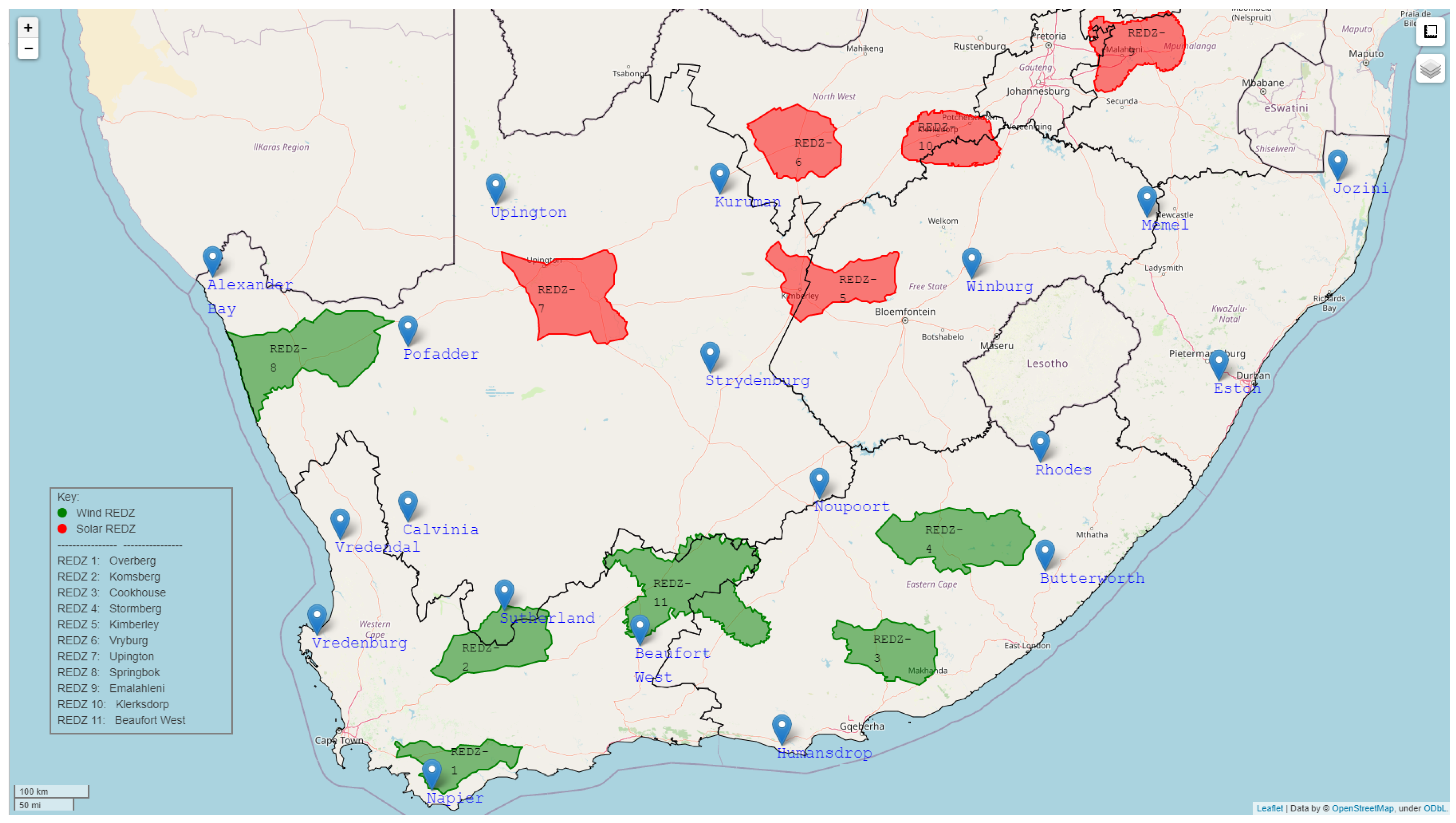
Among the eleven REDZs discussed in Section 2.1.1, six REDZs (presented by green in Figure 2) were chosen for the application and their respective wind data were obtained from WASA wind masts, as shown in

Table 2. Wind REDZs with corresponding wind masts.

Wind REDZs	Overberg	Komsberg	Cookhouse	Stormberg	Springbok	Beaufort West
Wind Masts	Napier	Sutherland	Humansdrop	Butterworth	Pofadder	Beaufort West

.

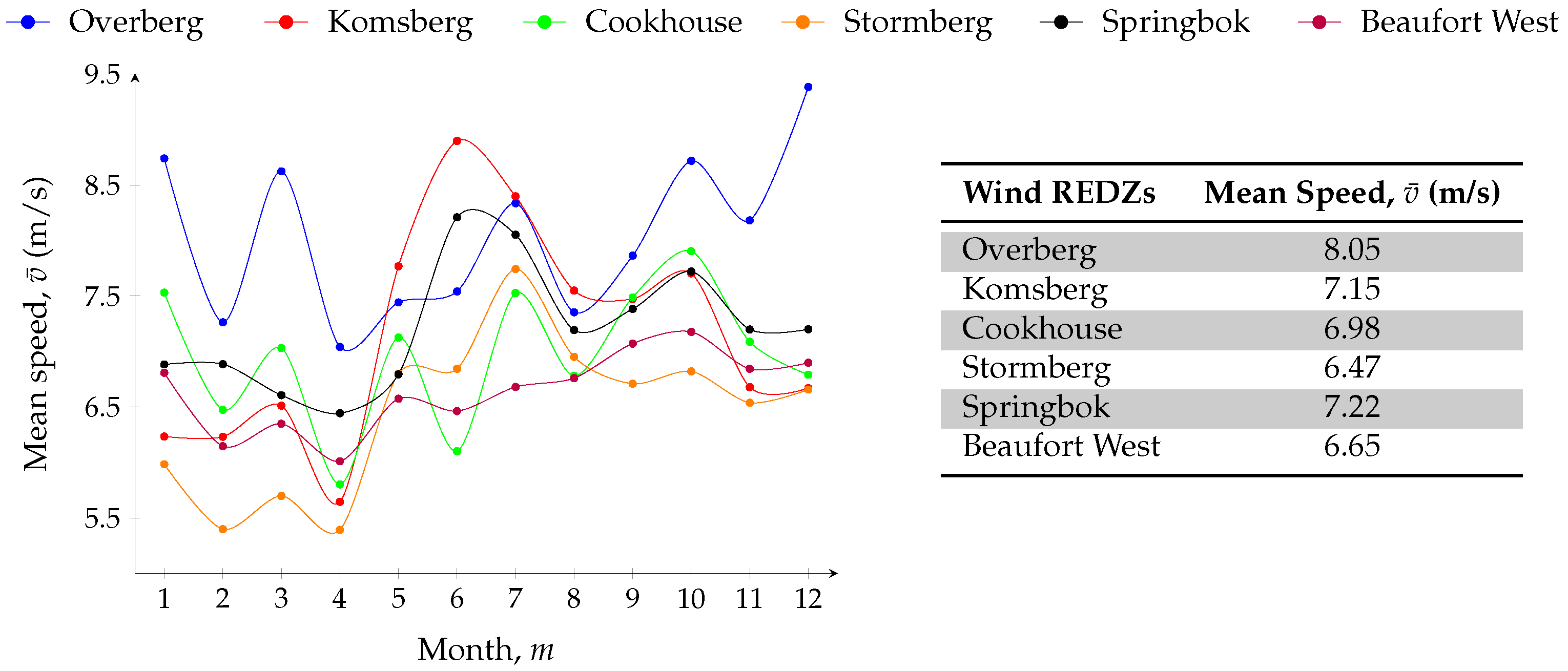
The latest 10 min wind speed data observed at anemometer height of 60 m for 2021 from wind masts are acquired and converted to 1 h average wind speed data by (1) with monthly and annual mean speed in (4) presented by Figure 7.

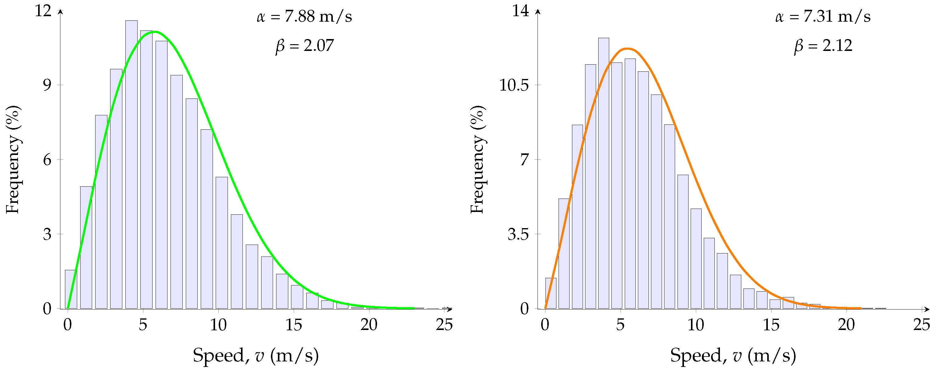
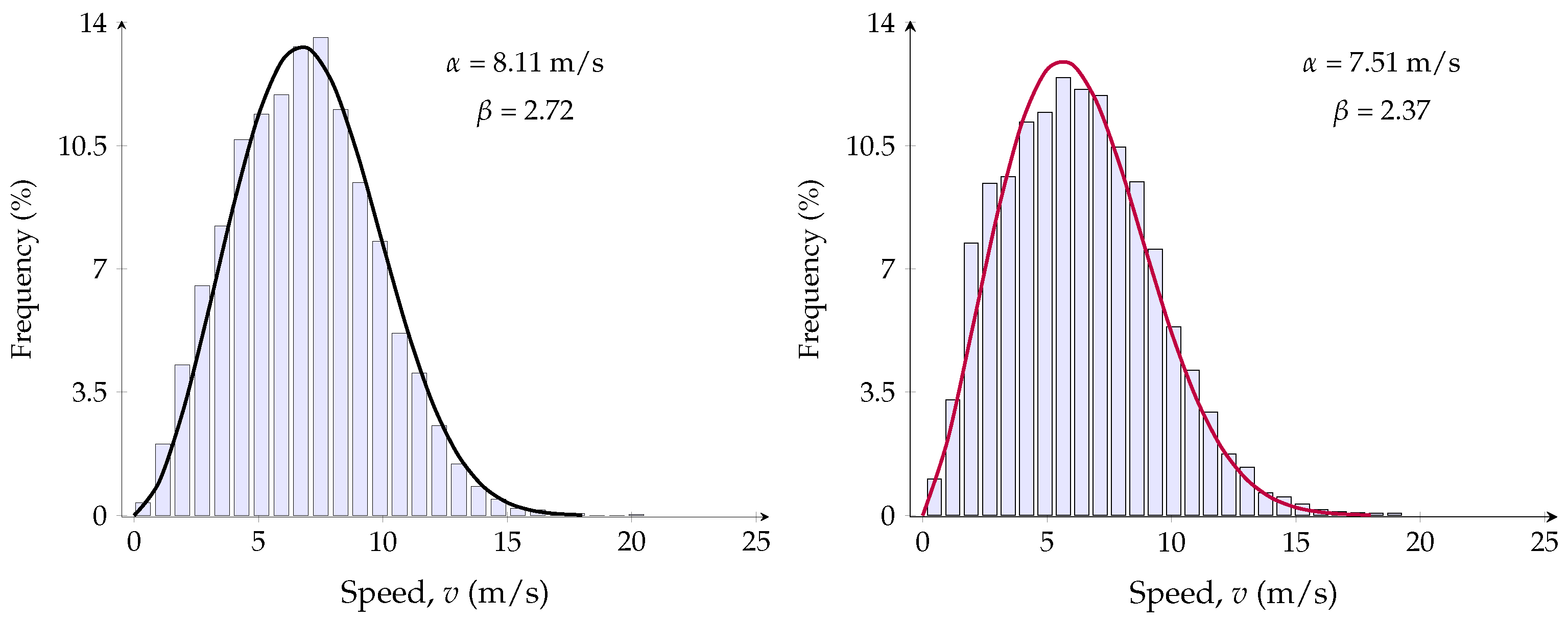
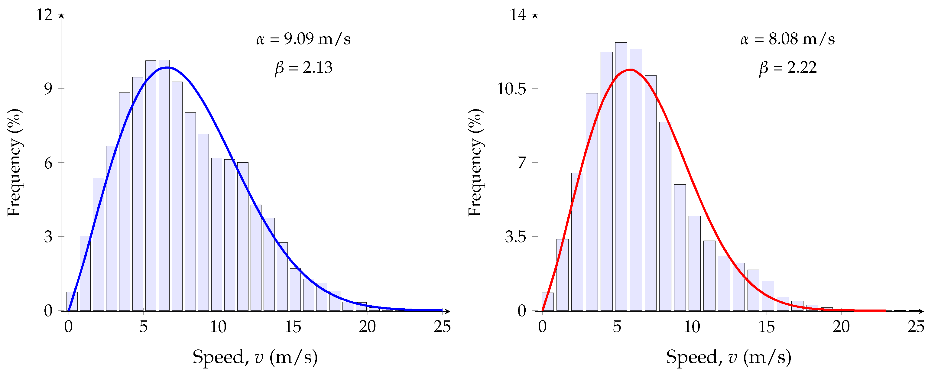
In Figure 7, Overberg has the highest annual mean speed, thus an expected high energy potential. Furthermore, Stormberg has the lowest annual speed, so the least energy production is expected. The wind speed frequency distribution of wind speed data using PDF in (2), with scale and shape parameters in (3) is obtained, as shown in Figure 8, Figure 9 and Figure 10 for all the six REDZs.

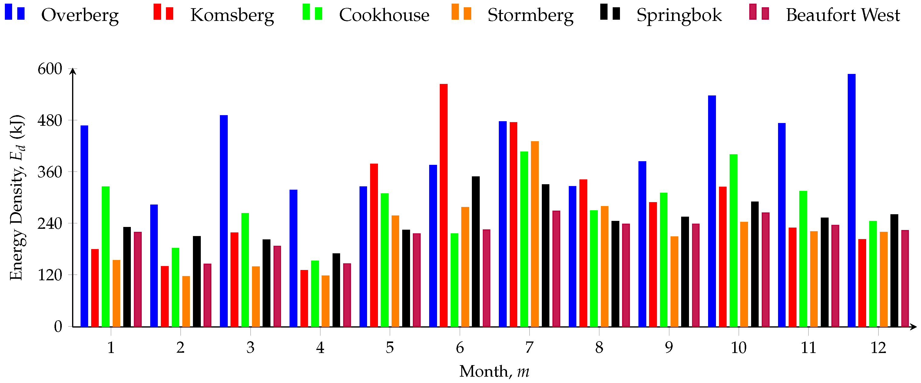
In Figure 8, Figure 9 and Figure 10, the occurrence frequency of different wind speeds for each wind REDZs is presented. Overberg, Komsberg and Springbok show the occurrence of high wind speeds, which is in agreement with the high annual mean speed in Figure 7 compared to Cookhouse, Stormberg and Beaufort West. Using the wind speed characteristics, the monthly energy density in (8) is determined in Figure 11.

In Figure 11, the highest energy density is noticed in Overberg, Komsberg and Springbok, and the lowest energy density in Cookhouse, Stormberg and Beaufort West, which is in accordance with their respective annual mean speeds in Figure 7.

Table 3. Annual energy density for the wind REDZs.

Wind REDZs
	Overberg	Komsberg	Cookhouse	Stormberg	Springbok	Beaufort West
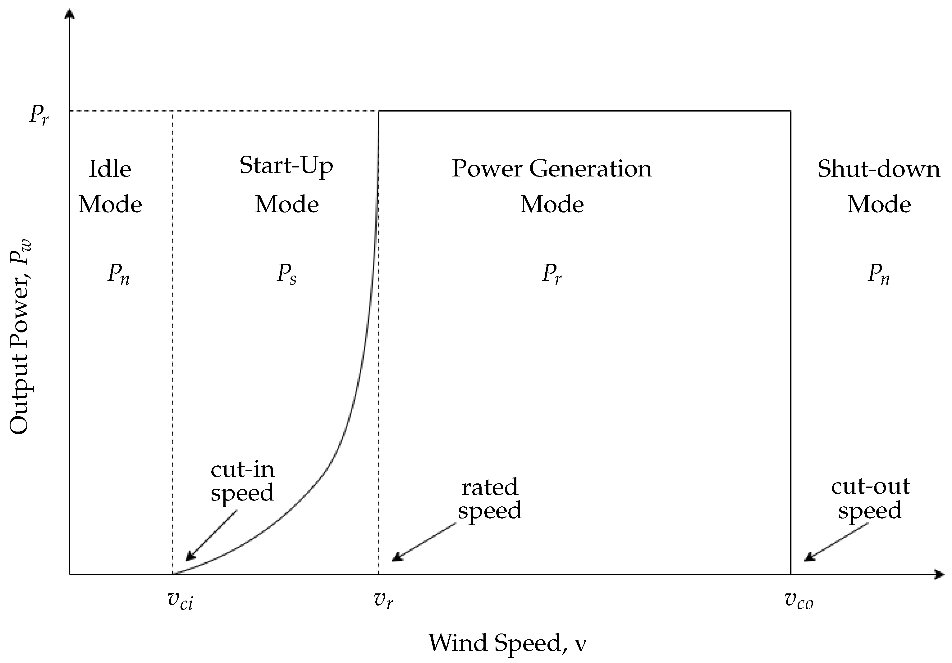
$E_d$ (kJ)	$5028.10$	$3411.02$	$3367.70$	$2623.00$	$3004.42$	$2593.17$

concludes that Overberg has the highest energy potential, and Beaufort West has the lowest energy potential of all wind REDZs as expected from their wind speed characteristics. For accuracy in energy assessment, the annual energy production of the REDZs is obtained using wind speed frequency characteristics in conjunction with an appropriate wind turbine model for the respective wind REDZs. Therefore, the optimal wind turbine variables, cut-in speed, $v_{ci}$, rated speed, $v_r$, cut-out speed, $v_{co}$, rotor diameter, $r_d$, and the hub height, $h_h$, are required.

A scope of wind turbine models from Nordex (N), DeWind (D), Vestas (V) and Gamesa (G) manufactures are shown in

Table 4. Wind turbine models.

Wind Turbine Model	${\mathit{P}}_{\mathit{r}}$ (kW)	${\mathit{v}}_{\mathit{ci}}$ (m/s)	${\mathit{v}}_{\mathit{r}}$ (m/s)	${\mathit{v}}_{\mathit{co}}$ (m/s)	${\mathit{r}}_{\mathit{d}}$ (m)	${\mathit{h}}_{\mathit{h}}$ (m)
N43	600	$2.5$	$15.0$	$25.0$	$43.0$	$60.0,78.0$
D$4/48$	600	$2.5$	$11.5$	$22.0$	$48.0$	$60.0,70.0$
N50	800	$2.5$	$15.0$	$25.0$	$50.0$	$46.0,50.0,60.0,70.0$
G52	800	$4.0$	$13.0$	$25.0$	$52.0$	$44.0,55.0,65.0$
V54	850	$4.0$	$14.0$	$25.0$	$52.0$	$60.0,65.0,70.0,75.0,85.0$
G58	850	$3.0$	$12.5$	$25.0$	$58.0$	$44.0,55.0,65.0$
N54	1000	$3.5$	$14.0$	$25.0$	$54.0$	$60.0,70.0$

to give an idea of the wind turbine variable ranges [21,22,26,39].

In cases where $h_h$ in Table 4 is different from the anemometer height, the wind speed at $h_h$, $v_h$, is calculated using (10) and (11) at anemometer heights of 62 m and 60 m, as discussed in Section 2.1.4. The calculated surface roughness coefficient, s (11) for each wind REDZ, is given in

Table 5. Surface roughness coefficient for the wind REDZs.

Wind REDZs
	Overberg	Komsberg	Cookhouse	Stormberg	Springbok	Beaufort West
s (-)	$0.16$	$0.13$	$0.22$	$0.11$	$0.15$	$0.11$

with expected values as discussed in [12].

The appropriate wind turbine model for each wind REDZ is selected by application of the optimization problem definition and procedure in Section 3 to ensure an optimal H-HES model in the next section.

4.2. Optimization Application and Results

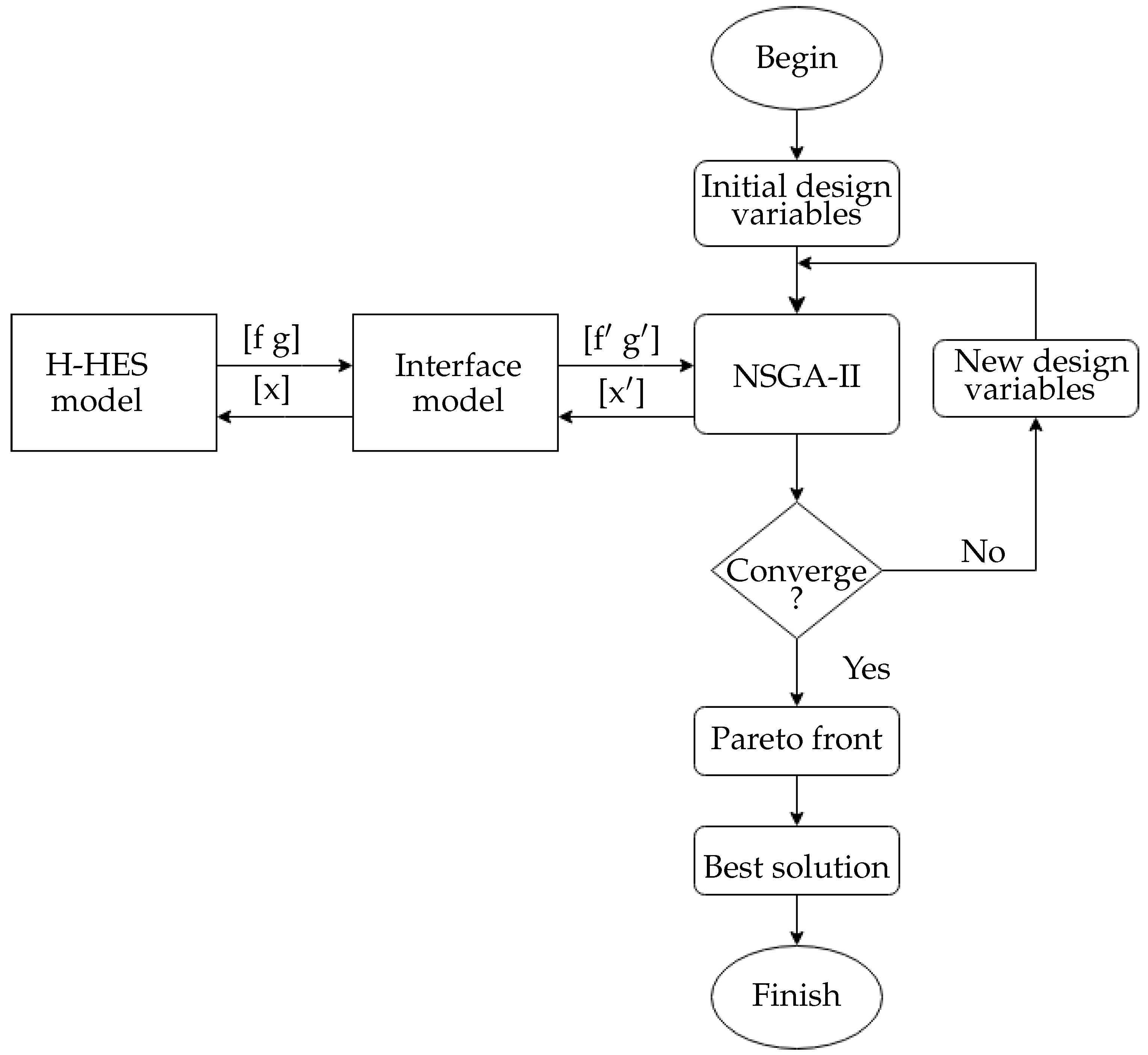
To implement the optimization procedure shown in Figure 6, the Pymoo framework, which offers NSGA-II, is utilized. Pymoo is chosen because it enables visualization of lower and upper-dimensional data, and can implement performance indicators to evaluate the quality of solutions from NSGA-II [33]. In addition, Pymoo provides a variety of multi-criteria decision-making tools that can be implemented after the NSGA-II has converged to a Pareto front to select the best solution in Figure 6.

The Pymoo framework only considers pure minimization of optimization problems. Therefore, objective functions to be maximized are multiplied by $-1$ to be minimized [33]. In addition, all constraint functions should be formulated as less than or equal to (⩽) zero. From (24), the design variables required to solve the objective and constraint functions are the variables on which the H-HES model depends. The chosen design variables include wind turbine variables (listed in Table 4) and H-HES model efficiencies: rotor (${\eta }_r$), gearbox (${\eta }_{gb}$), generator (${\eta }_{ge}$), EMS (${\eta }_{em}$) and rectifier (${\eta }_c$) and electrolyzer (${\eta }_e$) presented as:

$$\left[x\right]={[x_1{x}_2{x}_3{x}_4{x}_5{x}_6{x}_7{x}_8,x_9,x_{10},x_{11}]}^T={\left[r_d{h}_h{v}_{ci}{v}_r{v}_{co}{\eta }_r{\eta }_{gb}{\eta }_{ge}{\eta }_{em}{\eta }_c{\eta }_e\right]}^T$$

(26)

where the lower and upper bounds in (23) of each design variable are listed in

Table 6. Actual design variable boundaries.

Actual Design Variables
$40.0$ ≤ $r_d$ ≤ $60.0$
$60.0$ ≤ $h_h$ ≤ $90.0$
$2.5$ ≤ $v_{ci}$ ≤ $4.0$
12 ≤ $v_r$ ≤ $15.0$
$23.0$ ≤ $v_{co}$ ≤ $25.0$
$0.40$ ≤ ${\eta }_r$ ≤ $0.50$
$0.85$ ≤ ${\eta }_{gb}$ ≤ $0.95$
$0.90$ ≤ ${\eta }_{ge}$ ≤ $0.96$
$0.90$ ≤ ${\eta }_{em}$ ≤ $0.98$
$0.90$ ≤ ${\eta }_c$ ≤ $0.95$
$0.70$ ≤ ${\eta }_e$ ≤ $0.90$

.

In Table 6, the design variable bounds are according to Table 1, Section 2.3 and Section 2.4 and Table 4. Using design variables in (26), the cost of electricity, $C_e$, in (18) and efficiency, $\eta$, in (19) are minimized as:

$$\left[f\right]={\left[f_1{f}_2\right]}^T={\left[C_e\eta \right]}^T=\left[\begin{array}{c}{E}_g\tau \\ \\ -\left(\frac{P_w{\eta }_{em}{\eta }_c{\eta }_e}{P_k}\right)\end{array}\right].$$

(27)

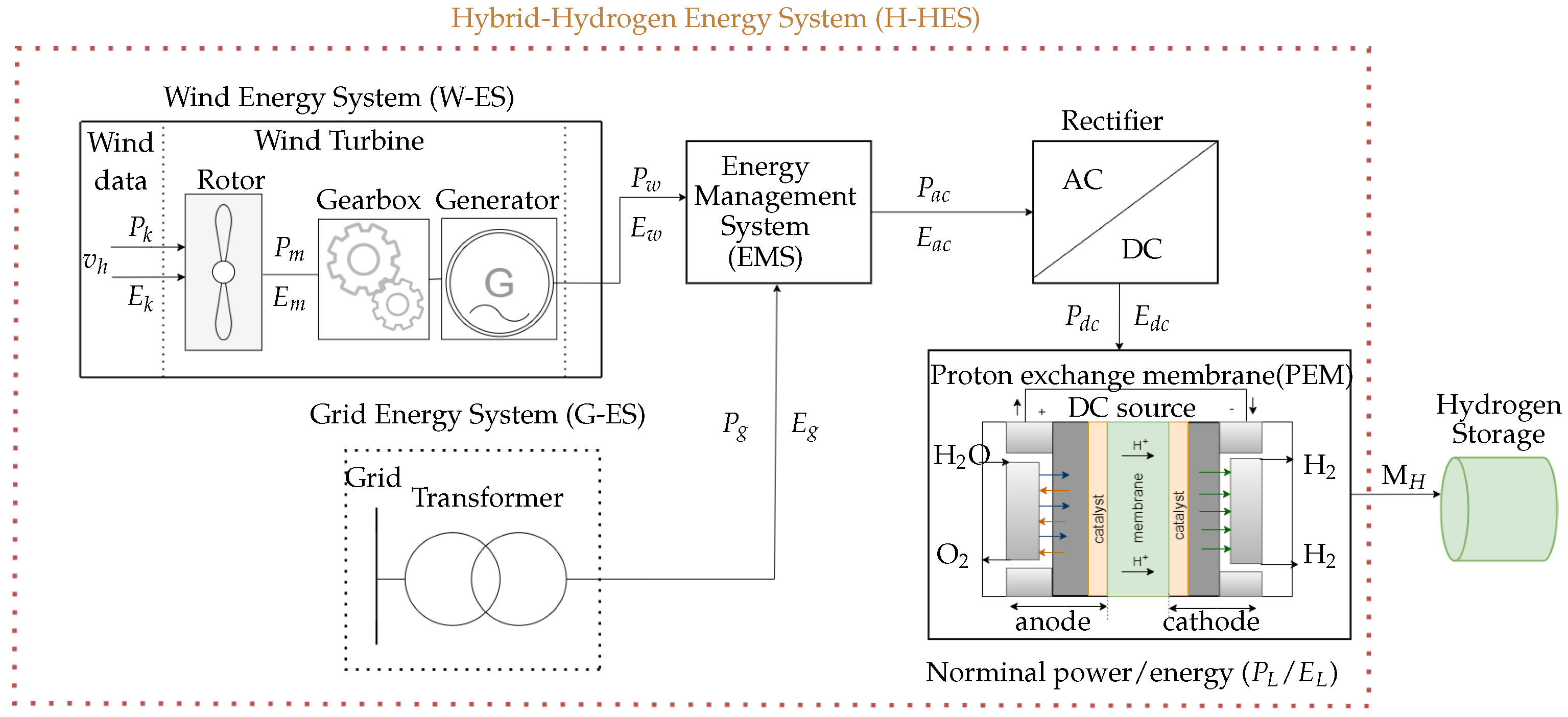
$C_e$ in (27) is calculated by Eskom tariff structure as discussed in Section 2.5. The Eskom tariff structure selected for $2022/2023$ based on Urban, Megaflex and non-local authority tariff charges, because the PEM electrolyzer in Figure 1 is connected directly to the substation, has a notified maximum demand greater than 1 MW and is within the Eskom supply area, respectively [38].

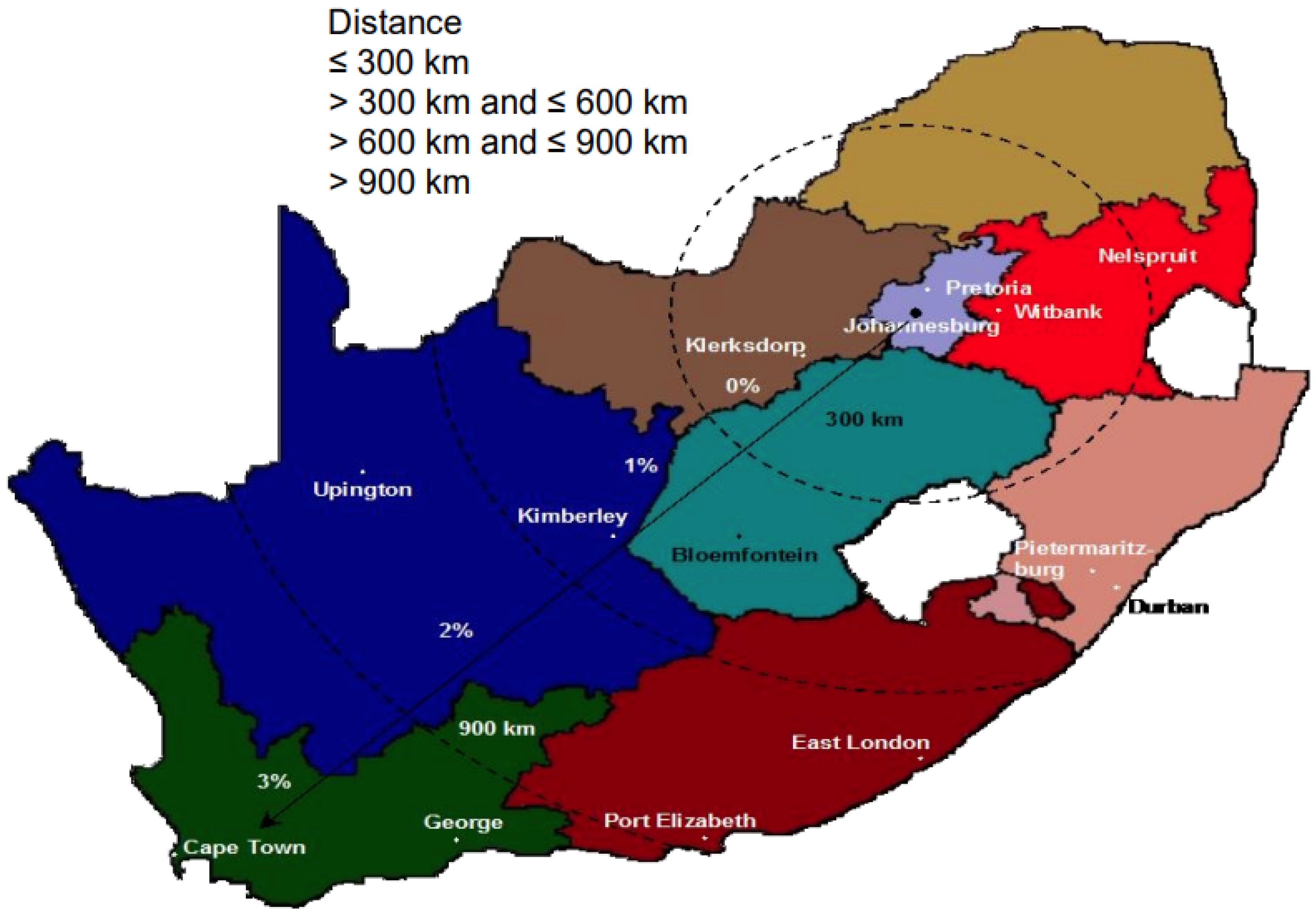
Using Figure 4, the transmission zones of the six wind REDZs in Table 2 and shown Figure 2 (in green) are concluded as >600 km and ≤900 km: Cookhouse, Stormberg and Beaufort West and >900 km: Overberg, Komsberg and Springbok. The transmission zones are listed in

Table 7. Urban Megaflex non-authority tariff charges (excluding VAT) [38].

Active Energy Charges (South African Rand (ZAR)/kWh)
		High Demand Season (Jun–Aug)			Low Demand Season (Sep–May)
Transmission Zone	Voltage	Peak	Standard	Off Peak	Peak	Standard	Off Peak
>600 km and ≤900 km	≥500 V and ≤66 kV	$4.5935$	$1.3917$	$0.7557$	$1.4984$	$1.0314$	$0.6543$
>900 km	≥500 V and ≤66 kV	$4.6392$	$1.4052$	$0.7628$	$1.5131$	$1.0412$	$0.6607$

including the assumed voltage level of the PEM electrolyzer.

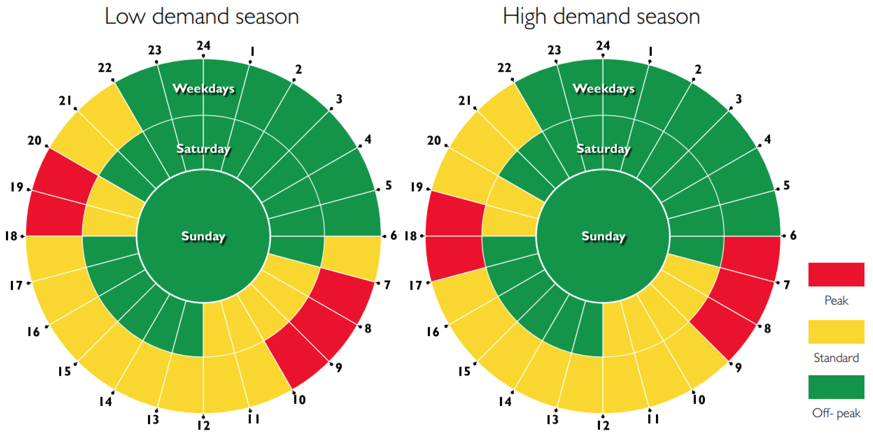
In addition, Table 7 gives active energy costs for TOU periods and demand seasons in Figure 5. The objective functions $C_e$ and $\eta$ in (27) are constrained by the nominal power or energy of the PEM electrolyzer. The PEM electrolyzer chosen for application is the H-TEC SYSTEMS because it offers mobility and reliability and can be scaled up for large-scale plants [40]. In

Table 8. Specifications of a 2 MW H-TEC PEM system [40].

Specification	Value
Electrical nominal power ($P_L$)	2 MW
H${}_2$ production	900 kg/day (420 Nm${}^3$/h)
H${}_2$ purity	$99.9$%
Energy consumption	$4.8$ kWh/Nm${}^3$ H${}_2$
System efficiency	74%

, 2 MW H-TEC PEM electrolyzer specifications are listed. The electrolyzer’s nominal power is the load, $P_L$, on which a load factor of $0.85$ is used. To give flexibility for NSGA-II to obtain the optimal solution, a constraint output range of $2.0$–$2.5$ MW is applied to get the nominal power of the electrolyzer.

Since the energy required by the electrolyzer (i.e., nominal energy, $E_L$) is known. $C_e$ for green H${}_2$ production assuming only the G-ES (shown in Figure 1) used is calculated using (18), with respect to the tariff charges for respective transmission zones in Table 7 of the REDZs, and given in

Table 9. Annual cost of electricity (only G-ES considered).

Wind REDZs	Cost of Electricity (ZAR million)
Overberg, Komsberg and Springbok	$22.8$
Cookhouse, Stormberg and Beaufort West	$22.6$

.

From Table 9, it can be concluded that the tariff charge increases with the transmission zone distance, as discussed in Section 2.5. With the design variables, objective and constraint functions are defined, NSGA-II is initialized with the operating parameters in

Table 10. NSGA-II operating parameters.

Optimization Parameters
Population size: 500
Number of offspring: 1000
Number of generations: 500
Sampling: Random
Mutation: Polynomial (Probability= $0.5$, index = 20)
Crossover: Simulated binary (Probability = $0.9$, index = 15)

to carry out the optimization procedure in Figure 6.

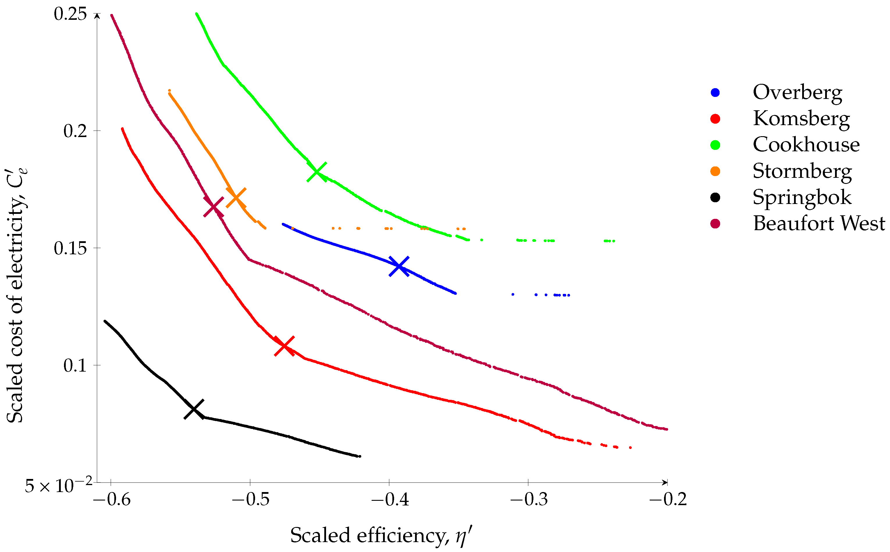
The number of generations in Table 10 is used for the convergence in optimization procedure shown in Figure 6 to obtain the scaled Pareto front solutions of objective functions, $\left[C_e^{\prime }{\eta }^{\prime }\right]$ in Figure 12. The execution time that NSGA-II takes to obtain solutions during the optimization process illustrated in Figure 6 is fast due to simple analytical equations used to model the H-HES in Section 2. Therefore, large population sizes and the number of generations can be adopted for improved accuracy.

The best solution selection is conducted only after the search for solution sets ends, thus NSGA-II has converged to a Pareto front. With the Pareto front (presented in Figure 12) known, the best solution is selected using multi-criteria decision-making techniques. However, before implementing the chosen technique, normalization of the objective functions is necessary due to different scales, as indicated by their different upper and lower bounds. Therefore, normalization ensures both objective functions equally dominate any distance evaluation in the objective space during the decision-making process [33].

After normalization, the compromise programming multi-criteria decision-making technique available in Pymoo is adopted due to its flexibility, as it employs any type of decomposition function. The augmented scalarization decomposition function is applied with an equal weight of both objective functions, resulting in the best solution (presented by X in Figure 12) for each wind REDZ.

The actual best solution of $\left[C_e\eta \right]$ passed to the H-HES model by interface model (as shown in Figure 6) for each REDZ is given in

Table 11. Actual best solutions of cost of electricity and efficiency from NSGA-II for wind REDZ.

	Wind REDZs
	Overberg	Komsberg	Cookhouse	Stormberg	Springbok	Beaufort West
$C_e$ (ZAR million)	$1.423$	$1.081$	$1.824$	$1.714$	$0.813$	$1.675$
$\eta$ (-)	$0.393$	$0.475$	$0.452$	$0.510$	$0.540$	$0.526$

.

It can be concluded that an optimal H-HES ensures cost savings when optimal design variables are utilized, as noted in Table 9 and Table 11. The cost of electricity in Table 9 is reduced by up to $90\%$ with the optimal H-HES model as given in Table 11 at maximum efficiency. Furthermore, from the optimal solutions of $C_e$ and $\eta$ in Table 11, the optimal design variables in (26) for each wind REDZ are given in

Table 12. Actual optimal design variables from NSGA-II.

Design Variables	Wind REDZs
	Overberg	Komsberg	Cookhouse	Stormberg	Springbok	Beaufort West
$r_d$ (m)	$40.0$	$40.8$	$40.0$	$45.0$	$40.6$	$42.0$
$h_h$ (m)	$60.3$	$65.4$	$85.0$	$89.0$	$79.0$	$68.8$
$v_{ci}$ (m/s)	$2.5$	$2.5$	$2.5$	$2.5$	$2.5$	$2.5$
$v_r$ (m/s)	$15.0$	$15.0$	$15.0$	$15.0$	$15.0$	$15.0$
$v_{co}$ (m/s)	$24.0$	$25.0$	$25.0$	$25.0$	$24.0$	$24.0$
${\eta }_r$ (-)	$0.50$	$0.50$	$0.50$	$0.50$	$0.50$	$0.50$
${\eta }_{gb}$ (-)	$0.95$	$0.95$	$0.95$	$0.95$	$0.95$	$0.95$
${\eta }_{ge}$ (-)	$0.92$	$0.96$	$0.96$	$0.96$	$0.95$	$0.96$
${\eta }_{em}$ (-)	$0.93$	$0.98$	$0.97$	$0.98$	$0.98$	$0.98$
${\eta }_c$ (-)	$0.95$	$0.95$	$0.95$	$0.95$	$0.95$	$0.95$
${\eta }_e$ (-)	$0.90$	$0.90$	$0.90$	$0.90$	$0.90$	$0.90$

.

For application purposes, the appropriate wind turbine model selected for all the wind REDZs is Nordex (N43) in Table 4, guided by the optimal variables in Table 12. Furthermore, using the PEM electrolyzer efficiency, ${\eta }_e$, in Table 8 and the optimal ${\eta }_r$, ${\eta }_{ge}$, ${\eta }_{gb}$, ${\eta }_{em}$ and ${\eta }_c$ efficiencies in Table 12, the recalculated $C_e$ and $\eta$ is given in

Table 13. Cost of electricity and efficiency using N43 wind turbine model for wind REDZs.

Wind REDZs
	Overberg	Komsberg	Cookhouse	Stormberg	Springbok	Beaufort West
$C_e$ (ZAR million)	$1.442$	$1.212$	$1.9028$	$1.824$	$0.8211$	$2.088$
$\eta$ (-)	$0.325$	$0.40$	$0.38$	$0.42$	$0.445$	$0.47$

.

In Table 13, the calculated $\left[C_e\eta \right]$ using appropriate wind turbine and optimal efficiencies is in close agreement with the best solutions from NSGA-II in Table 11. The calculated efficiency is slightly lower than the optimal efficiency, which is influenced by the efficiency ($74\%$) of the chosen PEM electrolyzer. It can be concluded that the optimal design variables have a great influence on the choice of wind turbine for each REDZ, hence an optimal H-HES model is successfully developed.

5. Conclusions

In the paper, a multi-objective optimization using a constrained optimization problem is employed to optimize H-HES model variables. The implementation and application of the optimization procedure with the cost of electricity and efficiency as objective functions are successfully demonstrated. The optimal costs of electricity and efficiency are achieved using the proposed optimization procedure, the optimal H-HES variables are derived and the appropriate wind turbine model for the wind REDZs is chosen for optimal H-HES modelling.

The following conclusions can be drawn from the results:

-

The wind REDZs have a high average wind speed (above 6 m/s), therefore, this is an indication of the high potential for green H${}_2$ production.

-

The knowledge of wind speed characteristics in conjunction with the appropriate wind turbine model successfully present the energy production potential of the wind REDZs.

-

The developed H-HES model is successfully demonstrated.

-

The open-source Pymoo module is a powerful tool that can be used in conjunction with NSGA-II to obtain optimal solutions free of charge.

-

The proposed H-HES interface models ensured that NSGA-II successfully converged to a Pareto front of the cost of electricity and efficiency for all the wind REDZs.

-

The optimal cost of electricity and efficiency successfully determine the required optimal variables to model the H-HES.

-

The derived optimal variables found for each wind REDZs greatly influence the choice of an appropriate wind turbine model for the W-ES and efficiencies of the H-HES, resulting in an optimal H-HES model.

-

The proposed optimal H-HES model can be adapted for green hydrogen production to ensure minimum cost (from the G-ES) at maximized efficiency with appropriate wind turbine model selection.