

Liquid Air Energy Storage Model for Scheduling Purposes in Island Power Systems

Abstract
:1. Introduction
2. Methodology
2.1. UC Formulation
2.2. Liquid Air Energy Storage (LAES)
2.2.1. LAES Model
2.2.2. LAES Basic Formulation
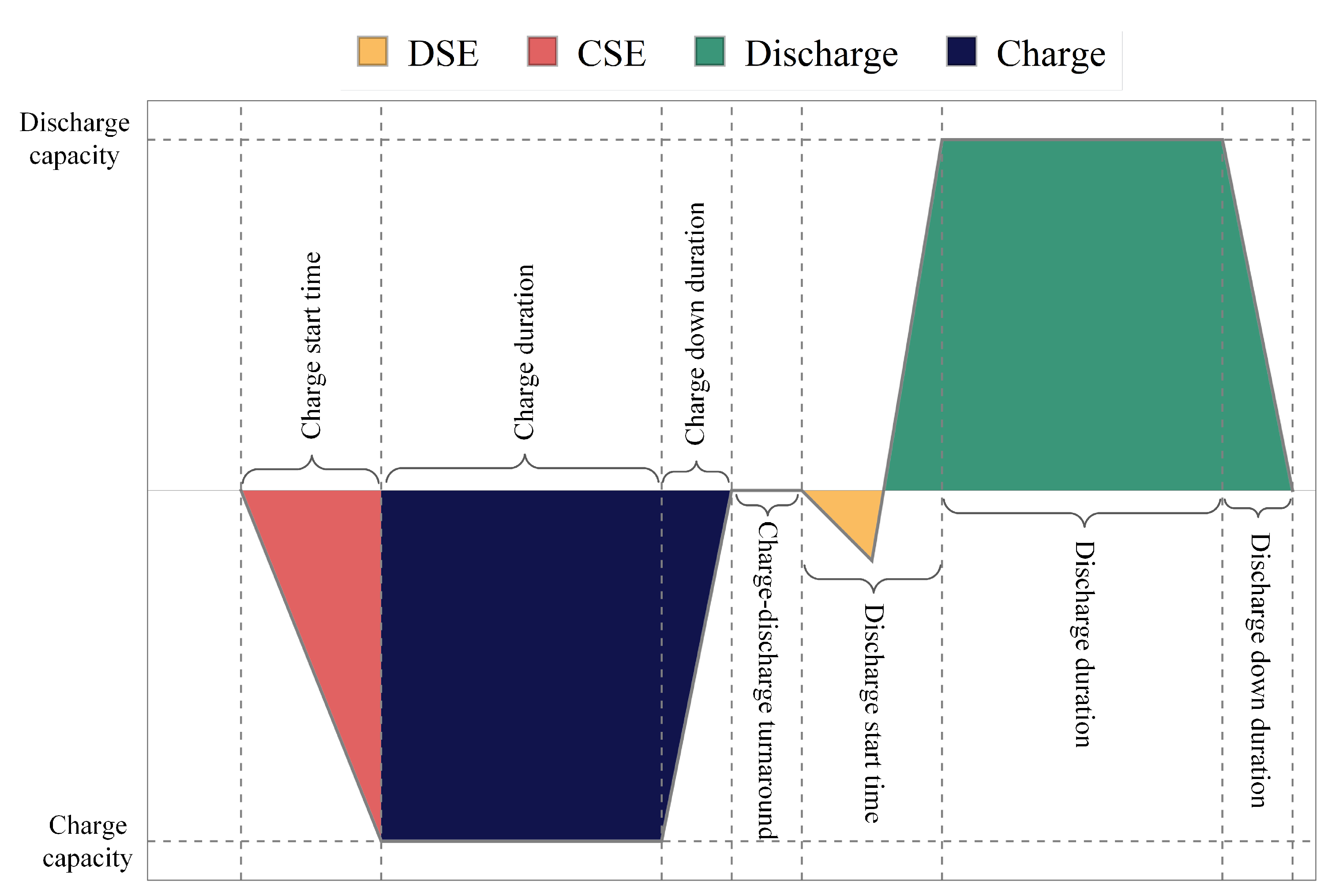
2.2.3. LAES Proposed Formulation
3. Results
- No LAES (base case): There is no LAES and no BESS in this scenario. It serves as the base case.
- A 50 MW LAES, basic model (50 MW BM): In this scenario, LAES with 50 MW/h maximum charging capacity and 300 MWh energy capacity is installed in the system, which is supported by a 50 MWh energy capacity BESS. The BESS only provides reserve. The basic LAES model is used in the formulation.
- A 50 MW LAES, the proposed model (50 MW PM): In this scenario, LAES with 50 MW/h maximum charging capacity and 300 MWh energy capacity is installed in the system, which is supported by a 50MWh energy capacity BESS. The BESS only provides reserve. The proposed LAES model is used in the formulation.
- A 100 MW LAES, basic model (100 MW BM): In this scenario, LAES with 100 MW/h maximum charging capacity and 600 MWh energy capacity is installed in the system, which is supported by a 100 MWh energy capacity BESS. The BESS only provides reserve. The basic LAES model is used in the formulation.
- A 100 MW LAES, the proposed model (100 MW PM): In this scenario, LAES with 100 MW/h maximum charging capacity and 600 MWh energy capacity is installed in the system, which is supported by a 100 MWh energy capacity BESS. The BESS only provides reserve. The proposed LAES model is used in the formulation.
4. Conclusions
Author Contributions
Funding
Informed Consent Statement
Data Availability Statement
Conflicts of Interest
Nomenclature
| Acronyms | |
| BESS | battery energy storage systems |
| CAES | compressed air energy storage |
| CHP | combined heat and power |
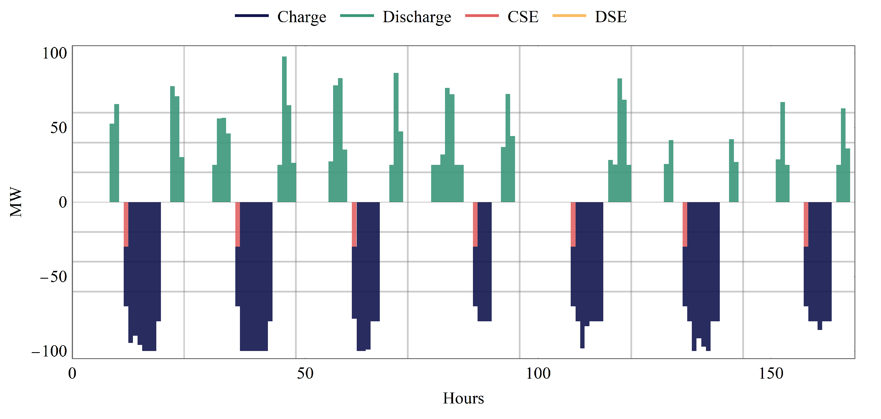
| CSE | charging start energy |
| CSP | charging start power |
| CST | charging start time |
| DSE | discharging start energy |
| DSP | discharging start power |
| DST | discharging start time |
| EES | energy storage system |
| HSS | hydrogen storage system |
| HTES | high-temperature thermal energy storage |
| IUC | interval unit commitment |
| LAES | liquid air energy storage |
| LNG | liquefied natural gas |
| MIL | mixed integer linear |
| PHES | pumped hydroelectric energy storage |
| PRD | primary response duration |
| RES | renewable energy source |
| RRM | renewable reserve multiplier |
| SMES | superconducting magnetic energy storage |
| UC | unit commitment |
| Indices | |
| i | index of generators |
| alias index for generators | |
| t | index of time intervals |
| alias index for time intervals | |
| Parameters | |
| power demand [MW] | |
| number of generators | |
| available solar [MW] | |
| time period | |
| available wind [MW] | |
| maximum power output of generator i [MW] | |
| LAES maximum charging [MW] | |
| LAES maximum discharging [MW] | |
| maximum ramp-up of generator i [MW] | |
| LAES minimum charging [MW] | |
| LAES minimum discharging [MW] | |
| minimum power output of generator i [MW] | |
| maximum ramp-down of generator i [MW] | |
| LAES round-trip efficiency | |
| minimum down-time of generators [hours] | |
| minimum up-time of generators [hours] | |
| Variables | |
| LAES energy state [MW] | |
| generation costs [€] | |
| p | thermal power generation [MW] |
| LAES charge power [MW] | |
| LAES discharge power [MW] | |
| r | online reserve power [MW] |
| BESS power reserve [MW] | |
| LAES power reserve [MW] | |
| thermal power reserve [MW] | |
| solar generation [MW] | |
| start-up costs [€] | |
| wind generation [MW] | |
| x | thermal unit status [∈{0,1}] |
| LAES charging status [∈{0,1}] | |
| LAES discharging status [∈{0,1}] | |
| y | thermal unit start-up [∈{0,1}] |
| LAES charging start-up [∈{0,1}] | |
| LAES discharging start-up [∈{0,1}] | |
| z | thermal unit shut-down [∈{0,1}] |
| LAES charging shut-down [∈{0,1}] | |
| LAES discharging shut-down [∈{0,1}] |
References
- Koohi-Fayegh, S.; Rosen, M.A. A review of energy storage types, applications and recent developments. J. Energy Storage 2020, 27, 101047. [Google Scholar] [CrossRef]
- Olabi, A.; Onumaegbu, C.; Wilberforce, T.; Ramadan, M.; Abdelkareem, M.A.; Al-Alami, A.H. Critical review of energy storage systems. Energy 2021, 214, 118987. [Google Scholar] [CrossRef]
- Wei, J.; Zhang, Y.; Wang, J.; Wu, L.; Zhao, P.; Jiang, Z. Decentralized Demand Management Based on Alternating Direction Method of Multipliers Algorithm for Industrial Park with CHP Units and Thermal Storage. J. Mod. Power Syst. Clean Energy 2022, 10, 120–130. [Google Scholar] [CrossRef]
- Borri, E.; Tafone, A.; Romagnoli, A.; Comodi, G. A review on liquid air energy storage: History, state of the art and recent developments. Renew. Sustain. Energy Rev. 2021, 137, 110572. [Google Scholar] [CrossRef]
- Menezes, M.V.P.; Vilasboas, I.F.; da Silva, J.A.M. Liquid Air Energy Storage System (LAES) Assisted by Cryogenic Air Rankine Cycle (ARC). Energies 2022, 15, 2730. [Google Scholar] [CrossRef]
- Mousavi, S.B.; Nabat, M.H.; Razmi, A.R.; Ahmadi, P. A comprehensive study and multi-criteria optimization of a novel sub-critical liquid air energy storage (SC-LAES). Energy Convers. Manag. 2022, 258, 115549. [Google Scholar] [CrossRef]
- Nabat, M.H.; Zeynalian, M.; Razmi, A.R.; Arabkoohsar, A.; Soltani, M. Energy, exergy, and economic analyses of an innovative energy storage system; liquid air energy storage (LAES) combined with high-temperature thermal energy storage (HTES). Energy Convers. Manag. 2020, 226, 113486. [Google Scholar] [CrossRef]
- Qi, M.; Park, J.; Kim, J.; Lee, I.; Moon, I. Advanced integration of LNG regasification power plant with liquid air energy storage: Enhancements in flexibility, safety, and power generation. Appl. Energy 2020, 269, 115049. [Google Scholar] [CrossRef]
- Park, J.; Cho, S.; Qi, M.; Noh, W.; Lee, I.; Moon, I. Liquid air energy storage coupled with liquefied natural gas cold energy: Focus on efficiency, energy capacity, and flexibility. Energy 2021, 216, 119308. [Google Scholar] [CrossRef]
- Gao, Z.; Ji, W.; Guo, L.; Fan, X.; Wang, J. Thermo-economic analysis of the integrated bidirectional peak shaving system consisted by liquid air energy storage and combined cycle power plant. Energy Convers. Manag. 2021, 234, 113945. [Google Scholar] [CrossRef]
- Hong, Y.Y.; Apolinario, G.F.D.; Lu, T.K.; Chu, C.C. Chance-constrained unit commitment with energy storage systems in electric power systems. Energy Rep. 2022, 8, 1067–1090. [Google Scholar] [CrossRef]
- Sedighizadeh, M.; Esmaili, M.; Mousavi-Taghiabadi, S.M. Optimal joint energy and reserve scheduling considering frequency dynamics, compressed air energy storage, and wind turbines in an electrical power system. J. Energy Storage 2019, 23, 220–233. [Google Scholar] [CrossRef]
- Nojavan, S.; Najafi-Ghalelou, A.; Majidi, M.; Zare, K. Optimal bidding and offering strategies of merchant compressed air energy storage in deregulated electricity market using robust optimization approach. Energy 2018, 142, 250–257. [Google Scholar] [CrossRef]
- Damak, C.; Leducq, D.; Hoang, H.M.; Negro, D.; Delahaye, A. Liquid Air Energy Storage (LAES) as a large-scale storage technology for renewable energy integration–A review of investigation studies and near perspectives of LAES. Int. J. Refrig. 2020, 110, 208–218. [Google Scholar] [CrossRef]
- Vecchi, A.; Li, Y.; Mancarella, P.; Sciacovelli, A. Integrated techno-economic assessment of Liquid Air Energy Storage (LAES) under off-design conditions: Links between provision of market services and thermodynamic performance. Appl. Energy 2020, 262, 114589. [Google Scholar] [CrossRef]
- REE. Estudios de Prospectiva del Sistema y Necesidades Para su Operabilidad; REE: Herzliya, Israel, 2020. [Google Scholar]


| 55% | |
|---|---|
| CST | 30 min |
| DST | min |
| CSE PM | |
| DSE | |
| Charge and discharge rundown time | 0 |
| Operation Cost (k€) | Scheduled RES (GW) | Number of Charging | Number of Discharging | |
|---|---|---|---|---|
| base case | 205,600 | 1877.3 | - | - |
| 50 MW BM | 181,215 | 1898.8 | 912 | 847 |
| 50 MW PM | 188,434 (+3.4%) | 1898.7 (0.0%) | 508 (−44.3%) | 834 (−1.5%) |
| 100 MW BM | 177,514 | 1900.4 | 847 | 769 |
| 100MW PM | 183,413 (+3.3%) | 1900.3 (0.0%) | 365 (−56.9%) | 730 (−5.1%) |
| Operation Cost (k€) | Scheduled RES (GW) | Number of Charging | Number of Discharging | |
|---|---|---|---|---|
| base case | 192,618 | 2127.7 | - | - |
| 50 MW BM | 168,753 | 2175.2 | 939 | 873 |
| 50 MW PM | 169,130 (+0.2%) | 2174.4 (−0.0%) | 560 (−40.4%) | 795 (−15.3%) |
| 100 MW BM | 162,647 | 2191.6 | 847 | 872 |
| 100 MW PM | 165,001 (+1.4%) | 2188.0 (−0.2%) | 469 (−44.6%) | 730 (−16.3%) |
| 50 MW BM (2026) | 100 MW BM (2026) | 50 MW BM (2030) | 100 MW BM (2030) | |
|---|---|---|---|---|
| Yearly CSE | 13,680 MW | 25,410 MW | 14,085 MW | 25,410 MW |
Publisher’s Note: MDPI stays neutral with regard to jurisdictional claims in published maps and institutional affiliations. |
© 2022 by the authors. Licensee MDPI, Basel, Switzerland. This article is an open access article distributed under the terms and conditions of the Creative Commons Attribution (CC BY) license (https://creativecommons.org/licenses/by/4.0/).
Share and Cite
Rajabdorri, M.; Sigrist, L.; Lobato, E. Liquid Air Energy Storage Model for Scheduling Purposes in Island Power Systems. Energies 2022, 15, 6958. https://doi.org/10.3390/en15196958
Rajabdorri M, Sigrist L, Lobato E. Liquid Air Energy Storage Model for Scheduling Purposes in Island Power Systems. Energies. 2022; 15(19):6958. https://doi.org/10.3390/en15196958
Chicago/Turabian StyleRajabdorri, Mohammad, Lukas Sigrist, and Enrique Lobato. 2022. "Liquid Air Energy Storage Model for Scheduling Purposes in Island Power Systems" Energies 15, no. 19: 6958. https://doi.org/10.3390/en15196958
APA StyleRajabdorri, M., Sigrist, L., & Lobato, E. (2022). Liquid Air Energy Storage Model for Scheduling Purposes in Island Power Systems. Energies, 15(19), 6958. https://doi.org/10.3390/en15196958