
Benchmarking Real-Time Control Platforms Using a Matlab/Simulink Coder with Applications in the Control of DC/AC Switched Power Converters

 ,
,  , , and
Abstract
:1. Introduction
2. Real-Time Control Platforms for Rapid Control Prototyping
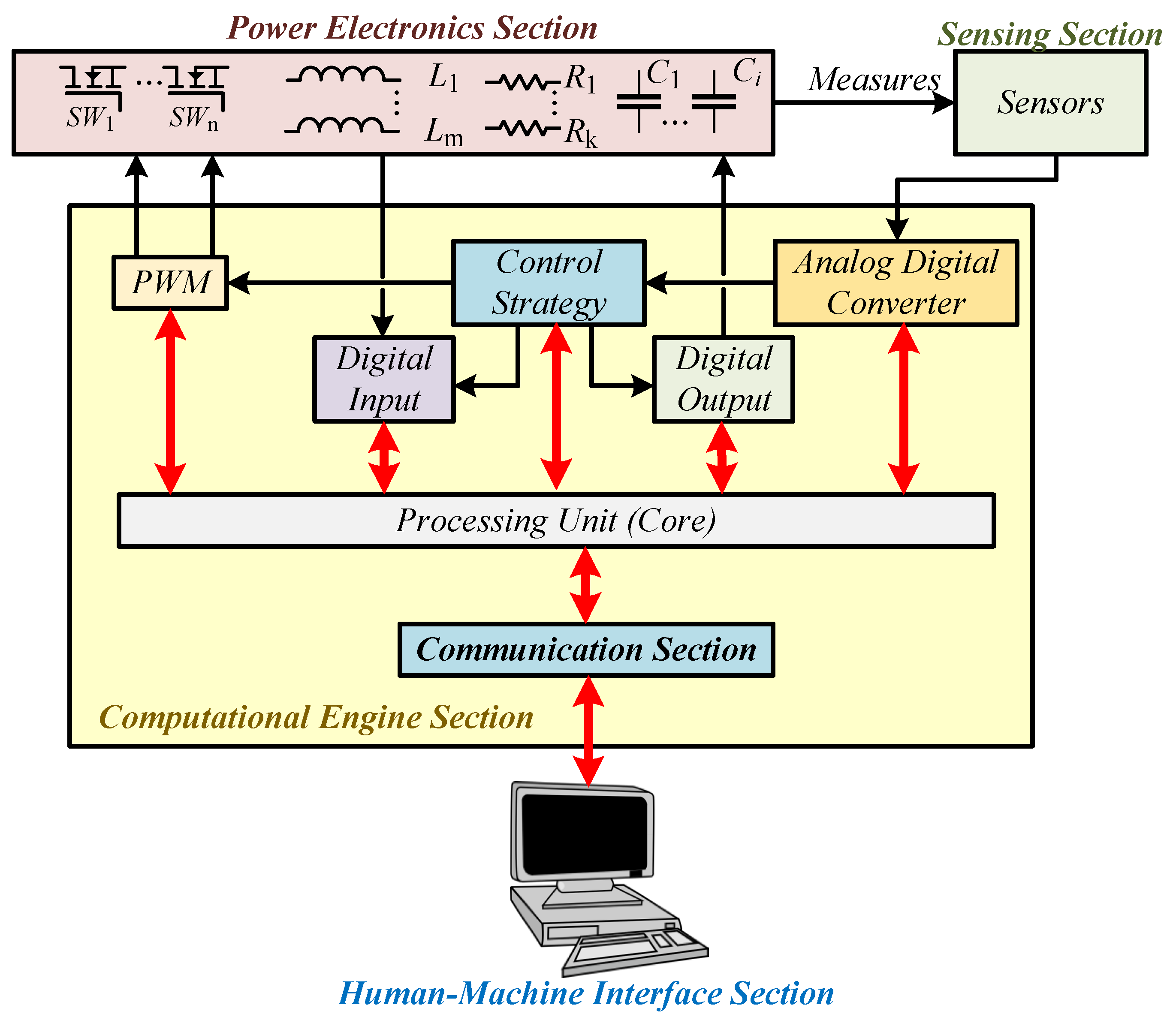
2.1. Technical Description of the RTCP
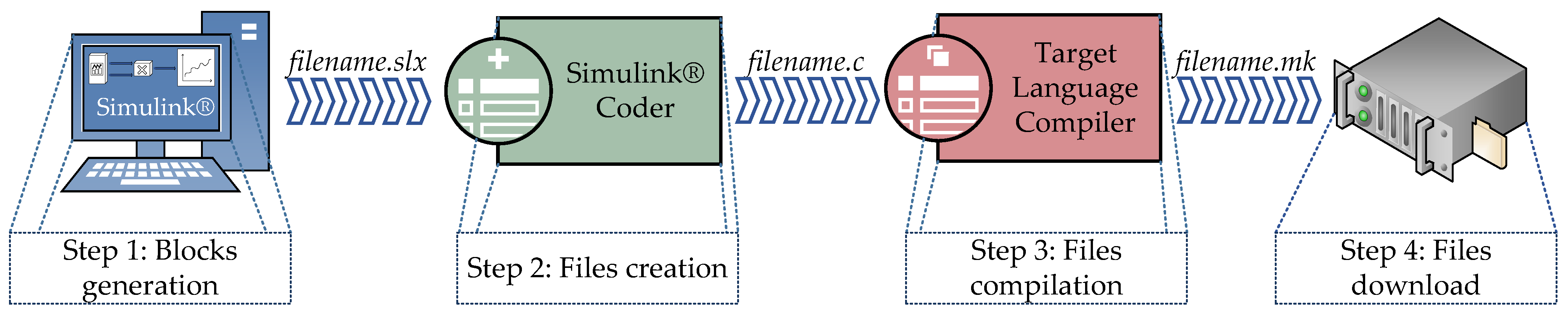
2.2. Code Generation Process
3. Controller Description
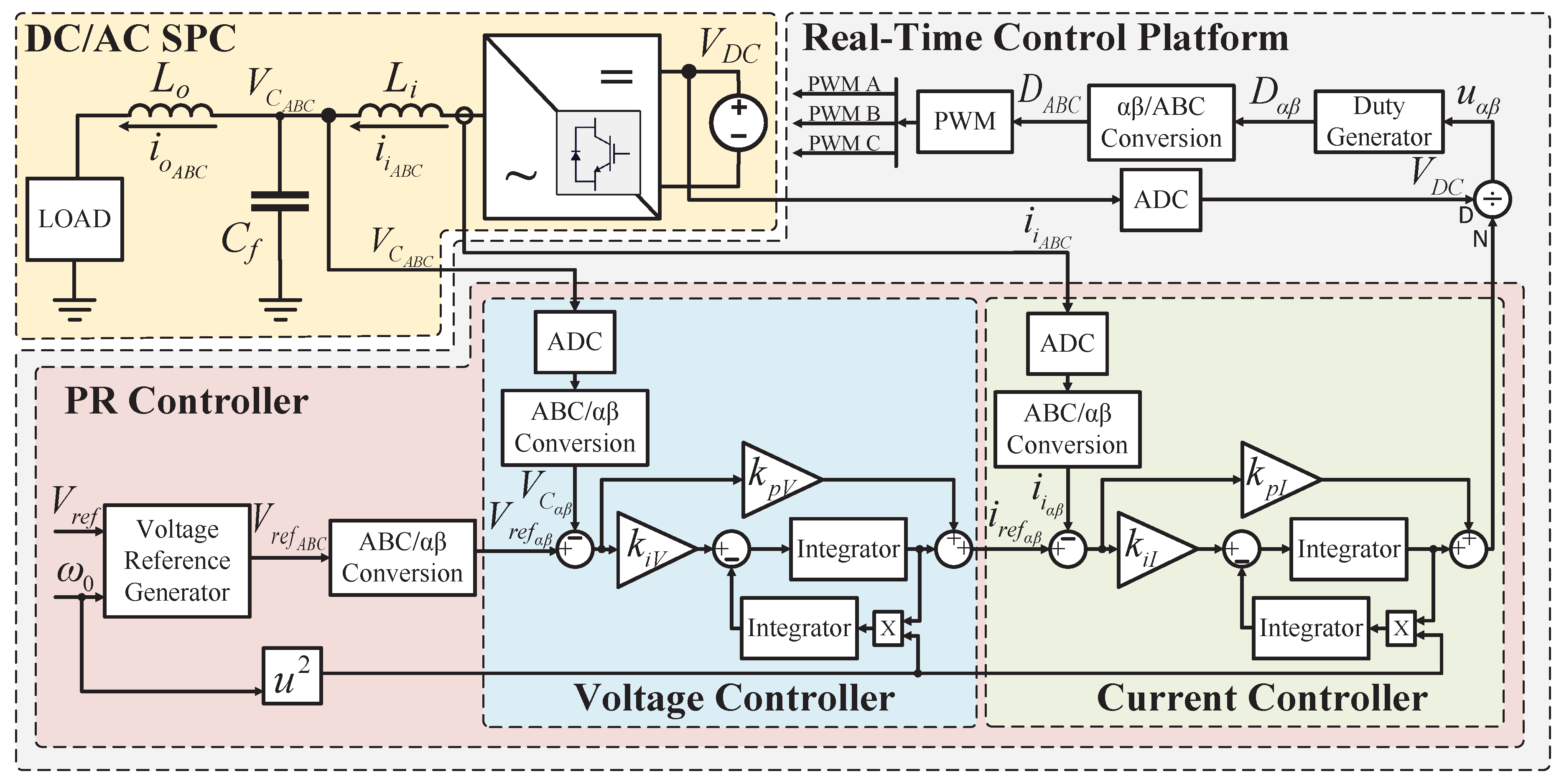
3.1. Proportional-Resonant (PR) Controller
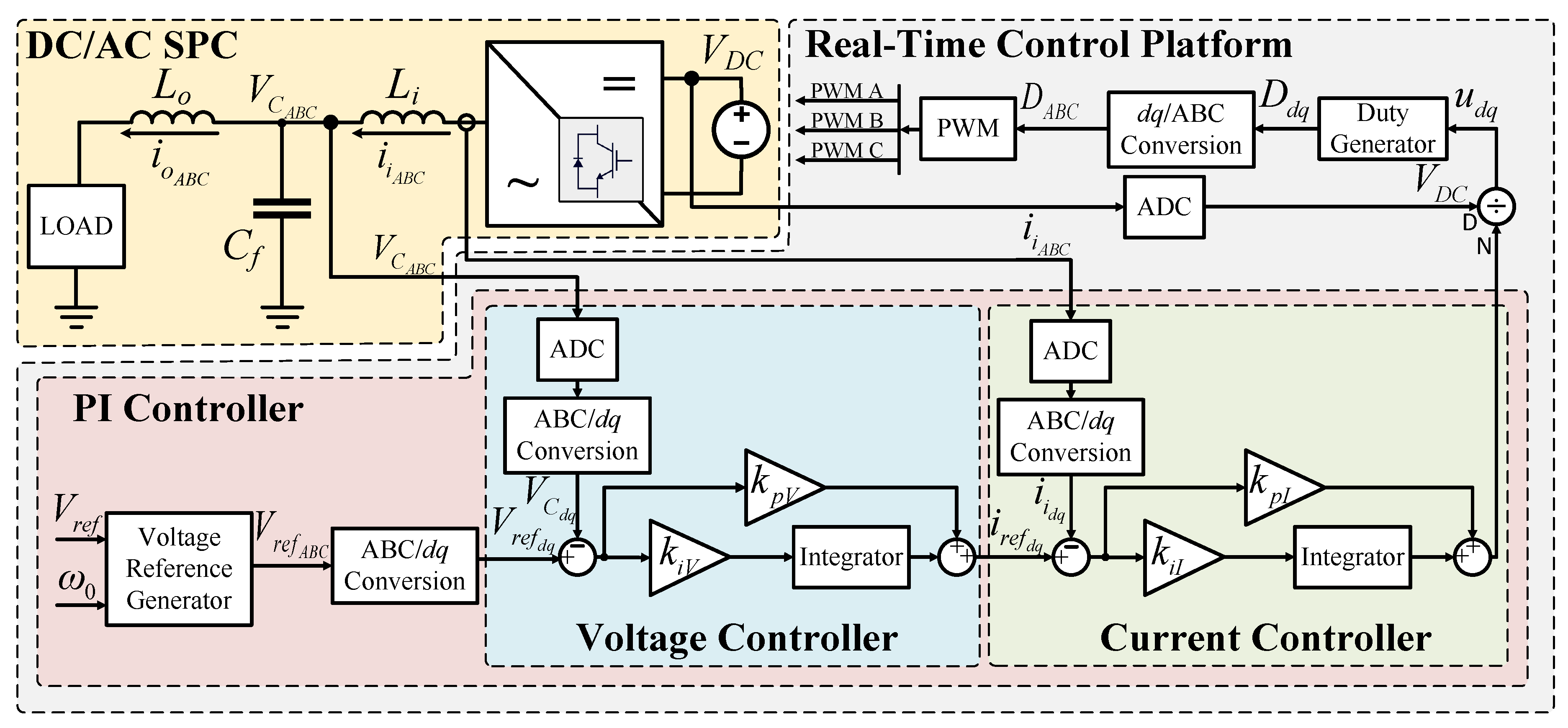
3.2. Proportional-Integral (PI) Controller
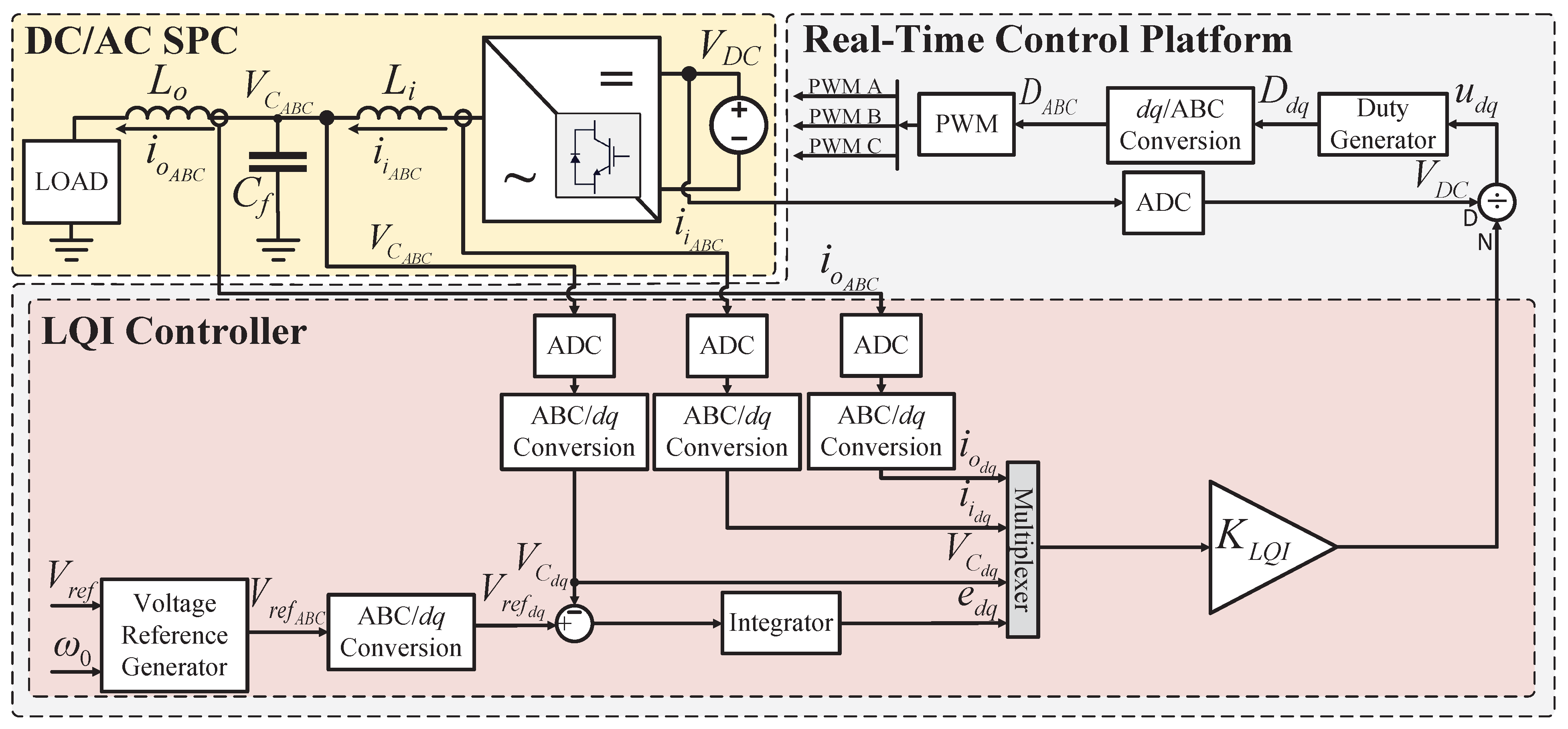
3.3. Linear-Quadratic-Integral (LQI) Controller
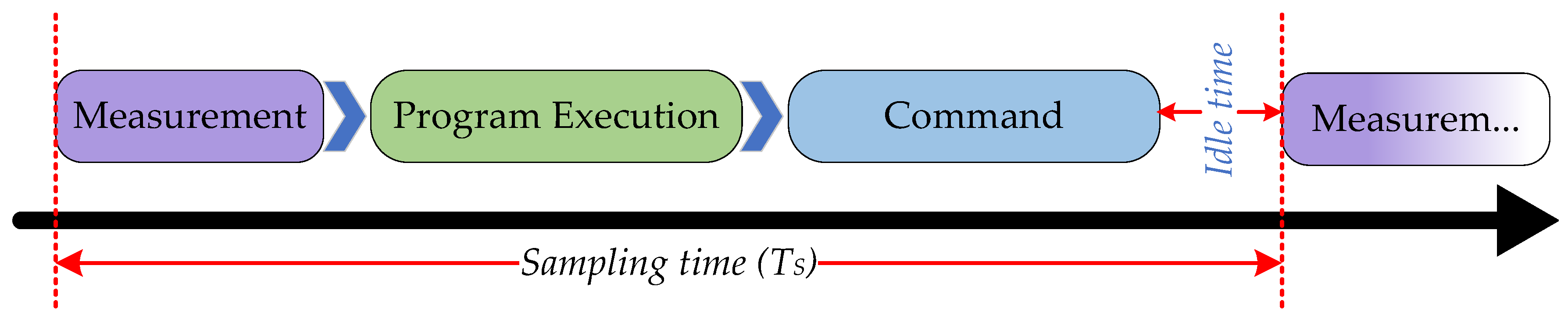
4. Methodology for the Measurement of Computation Time Profiles
- 1.
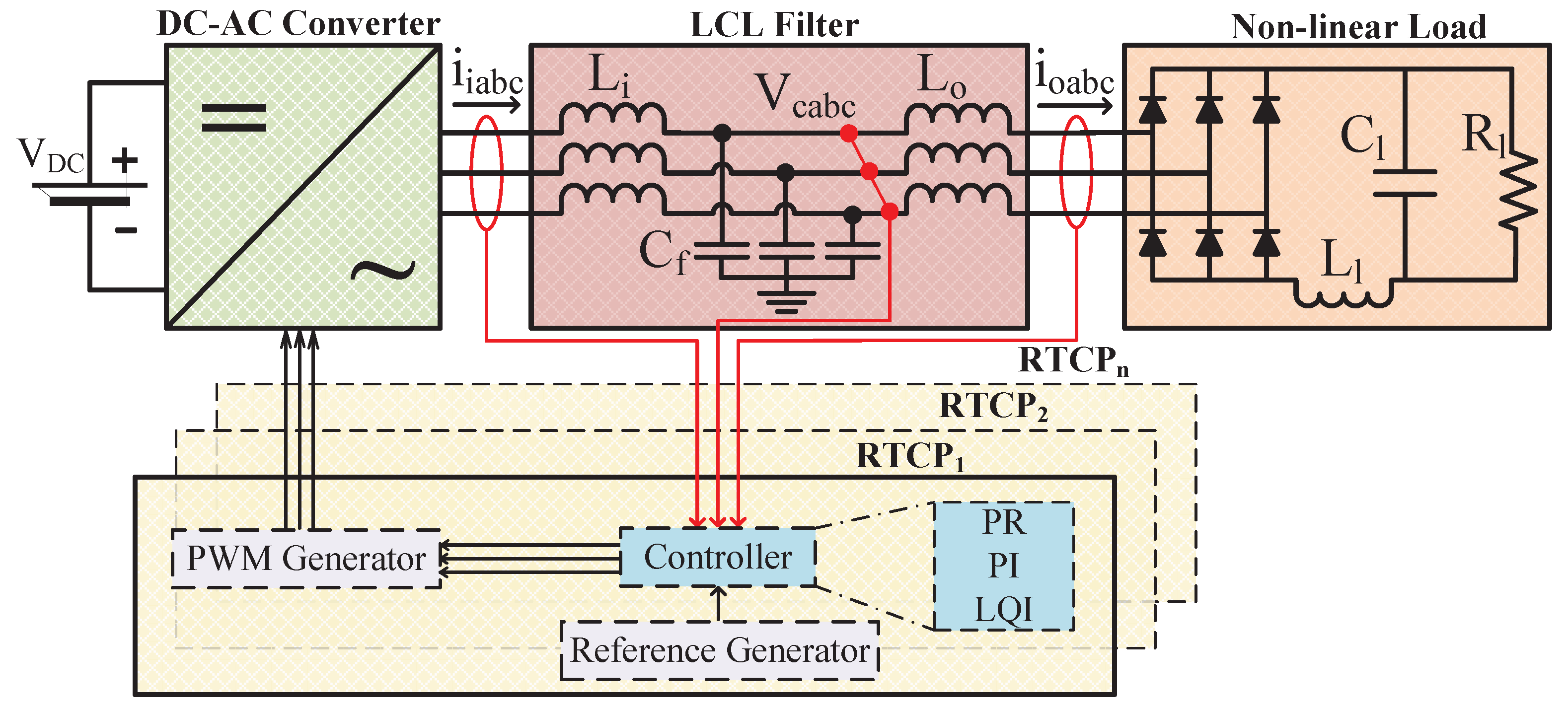
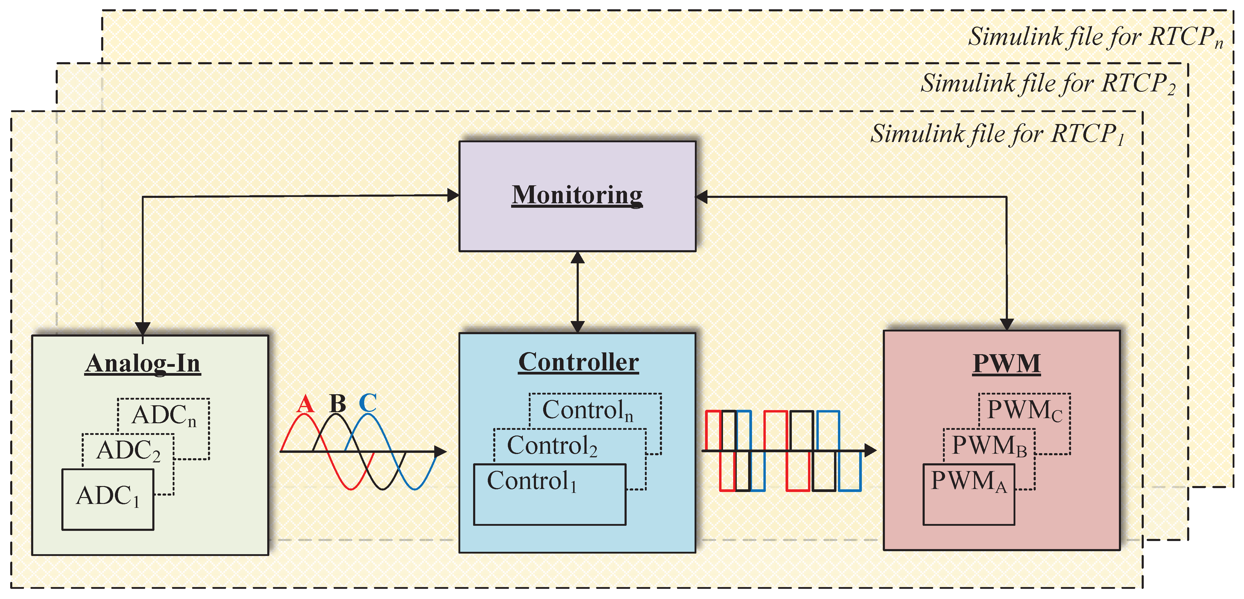
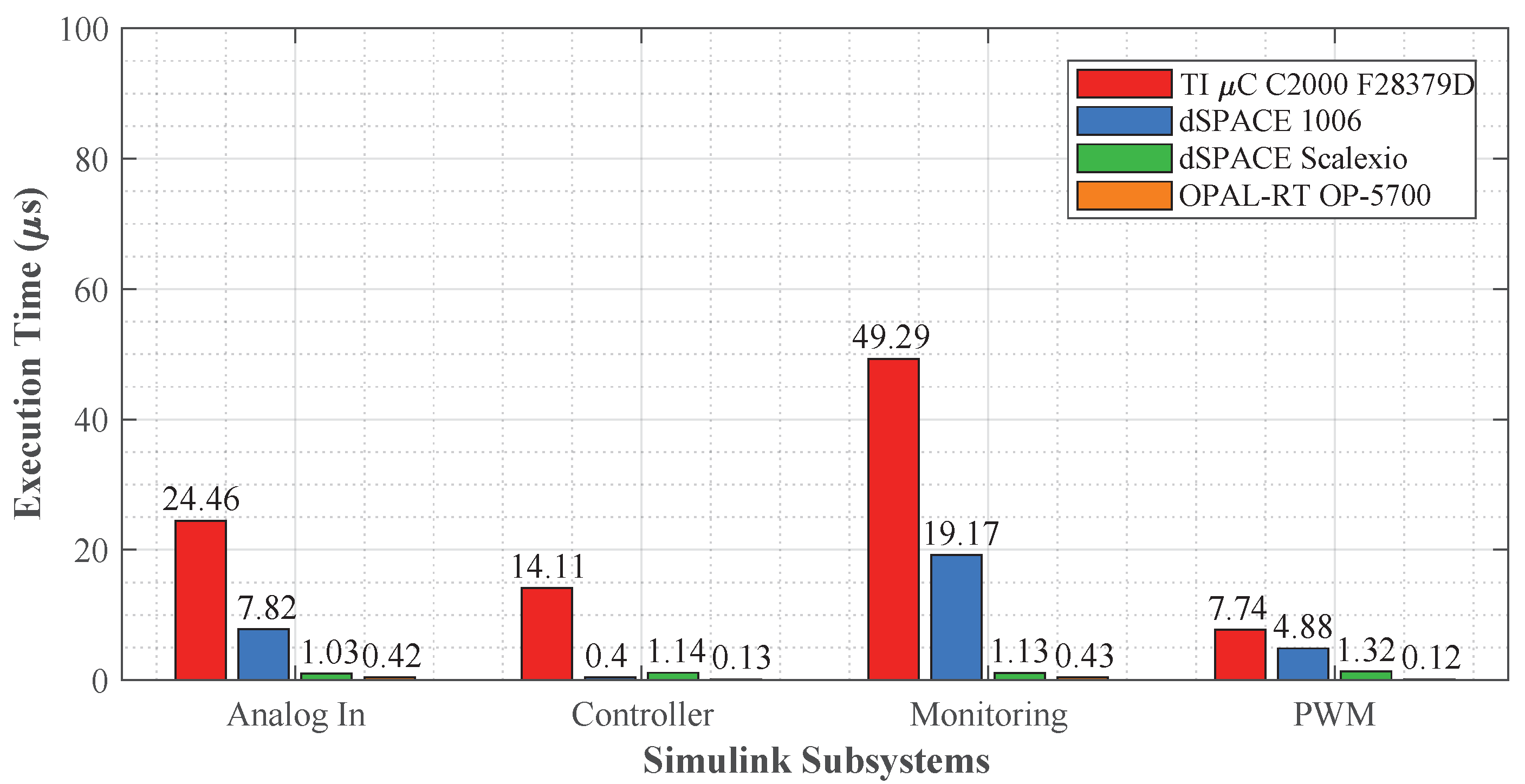
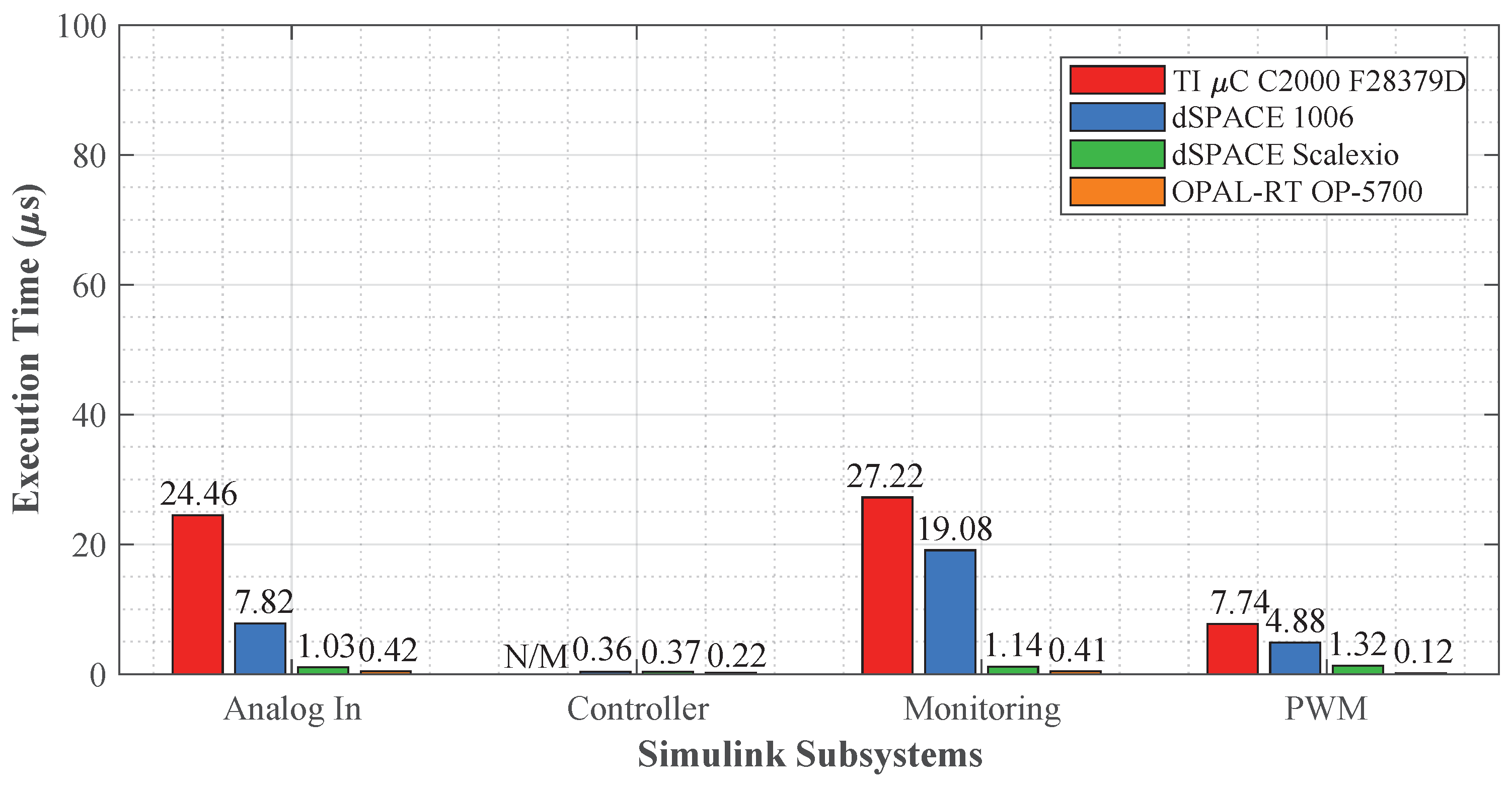
- The Analog-In subsystem contains the ADC reading blocks and the conditioning of the voltage and current signals that will be used by the Controller. These change according to the RTCP under test in terms of quantity, resolution and conversion time.
- 2.
- The Controller subsystem contains the control strategy and generates the control signals that the PWM subsystem will use. The content of this subsystem varies according to the control strategy used and is the same for all RTCPs.
- 3.
- The PWM subsystem holds the PWM blocks that generate the switching signals that go to the power electronics stage (see Figure 1). The amount of blocks in this subsystem varies according to the PWM block configuration of each RTCP.
- 4.
- Finally, the Monitoring subsystem contains the parameters that can be changed in real-time, such as the gains of the controllers, the frequency and the reference voltage for the DC/AC SPC. In addition, it holds the blocks for calculating the active-reactive power, voltage–current RMS and THD values.
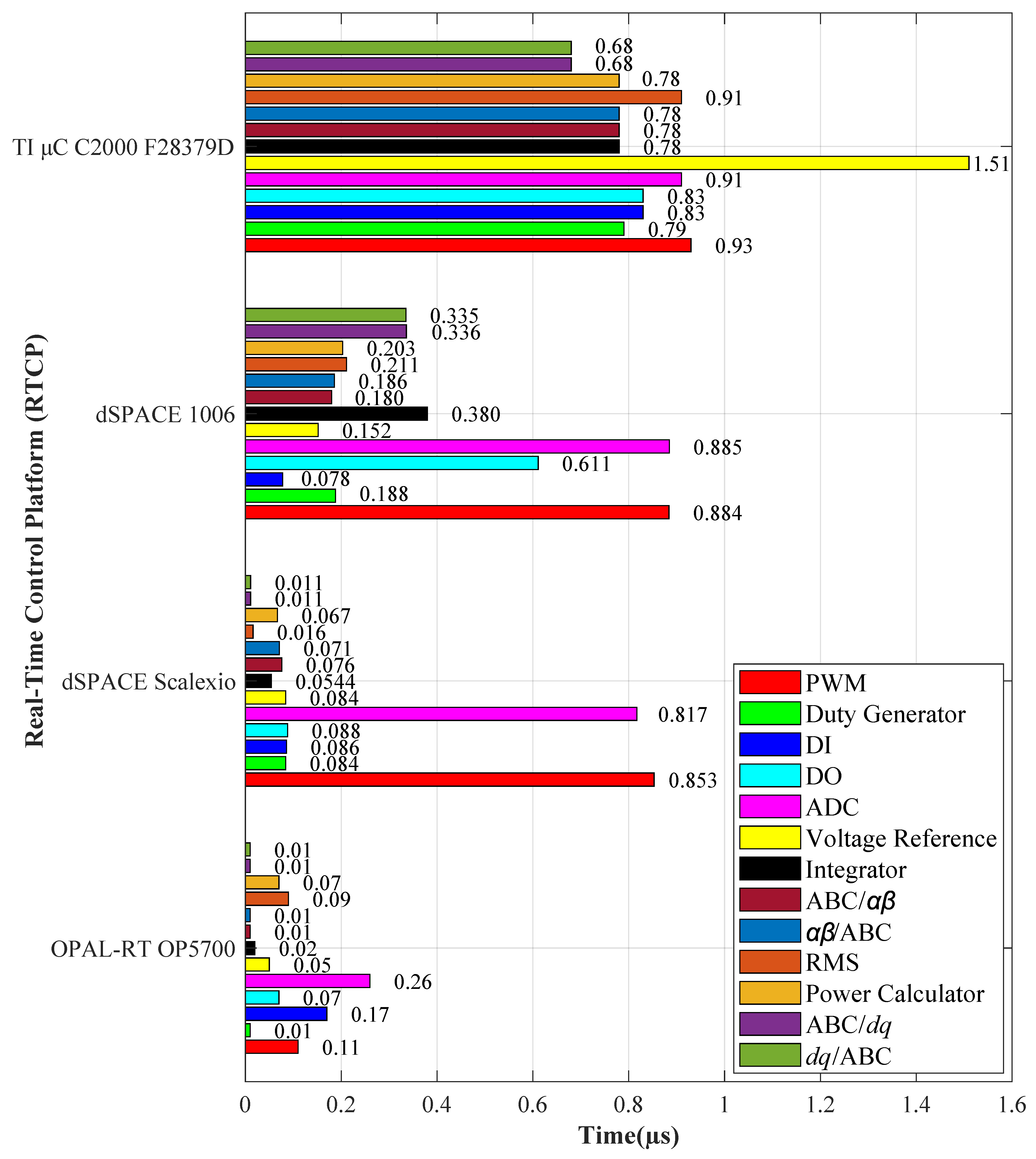
4.1. Matlab/Simulink Common Blocks in Real-Time Control of DC/AC SPC
4.2. Scenarios Designed to Compare RTCPs
4.2.1. Scenario 1: Voltage–Current Controllers
- The full version contained an instantaneous, three-phase active–reactive power calculation block with two first-order low pass filters and the RMS calculation blocks for the currents (, ) and the voltages () of the LCL filter (see Figure 4). In addition, it contained an error calculation block for .
- The debugged version only contained a block for calculating the RMS error of voltage and a block for calculating the RMS values of voltage .
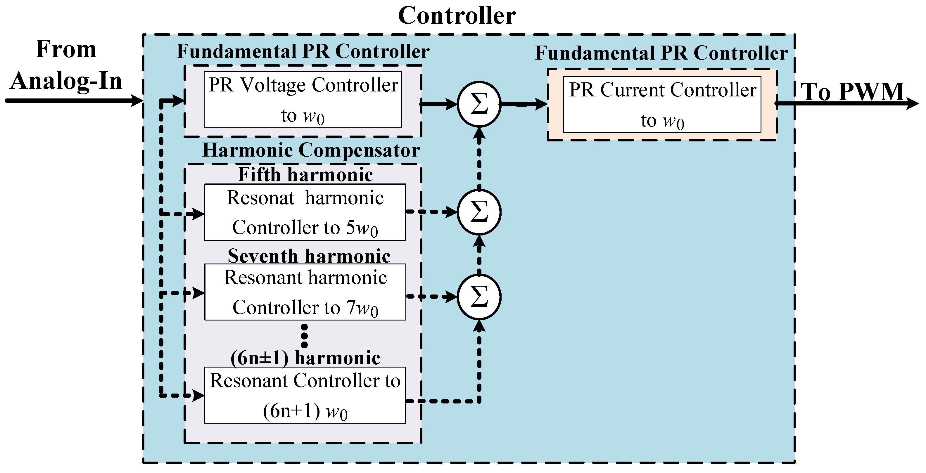
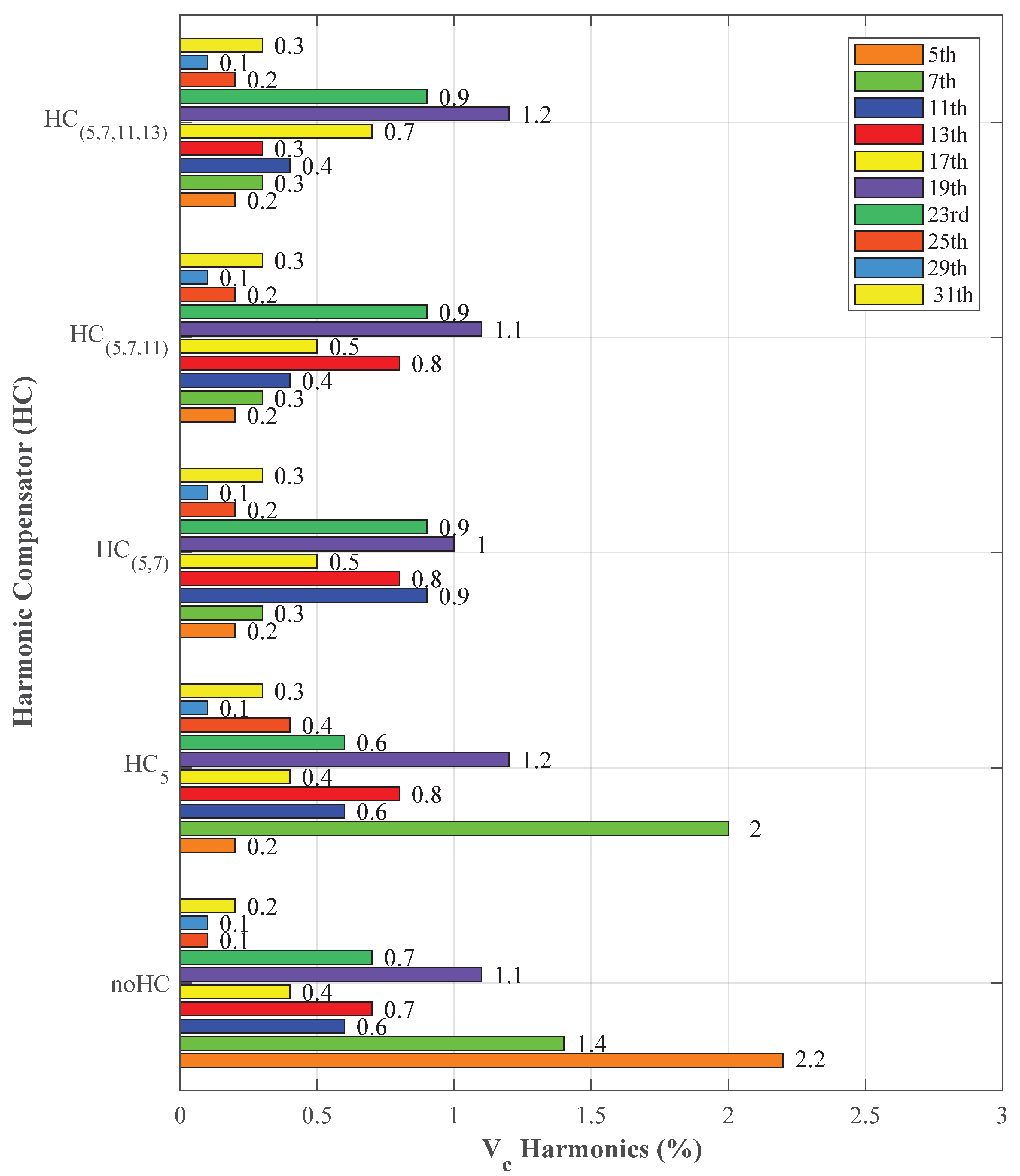
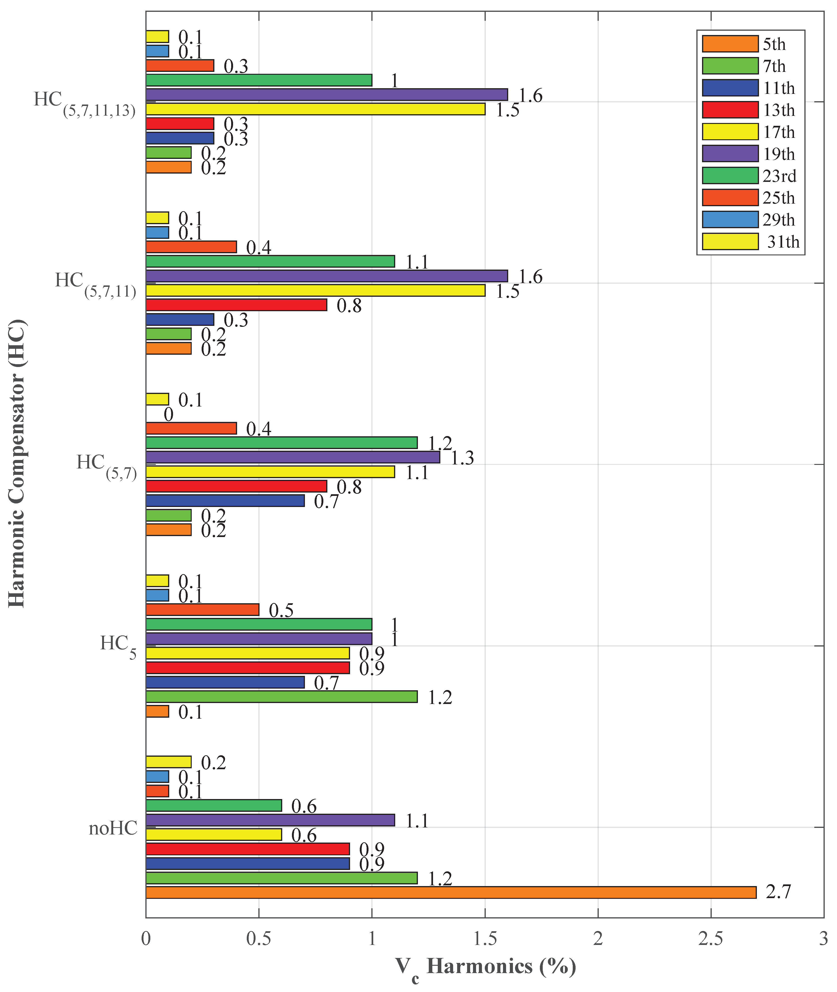
4.2.2. Scenario 2: Voltage Harmonic Controller
5. Computation Time Profile Measurement
5.1. Low-Cost C-Based RTCP
5.2. dSPACE Scalexio RTCP
5.3. dSPACE 1006 RTCP
5.4. OPAL-RT OP5700 RTCP
6. Experimental Results
6.1. Computation Time Profiles per Block
6.2. Scenario I: Computation Time Profiles for Voltage–Current Controllers
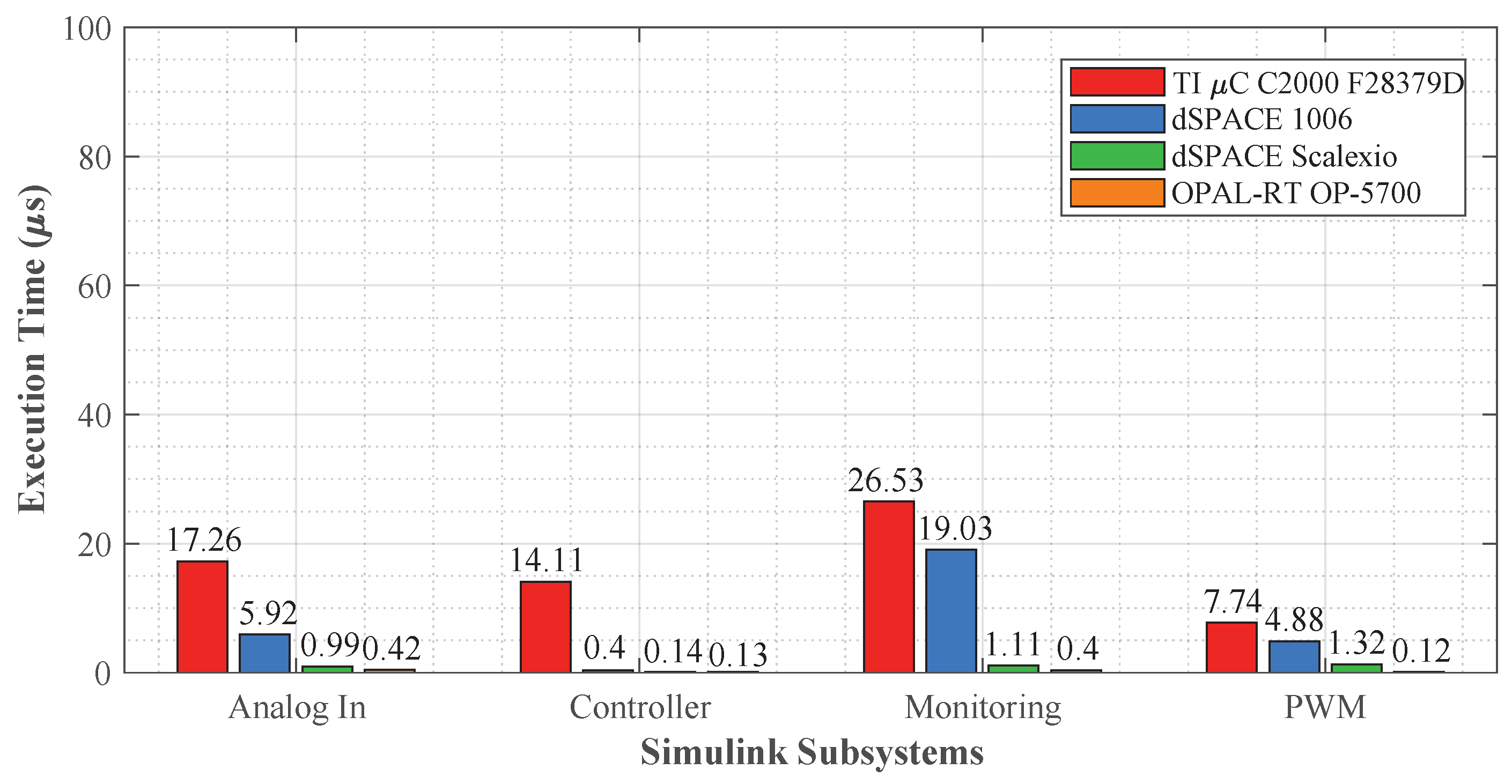
6.2.1. PR () Controller
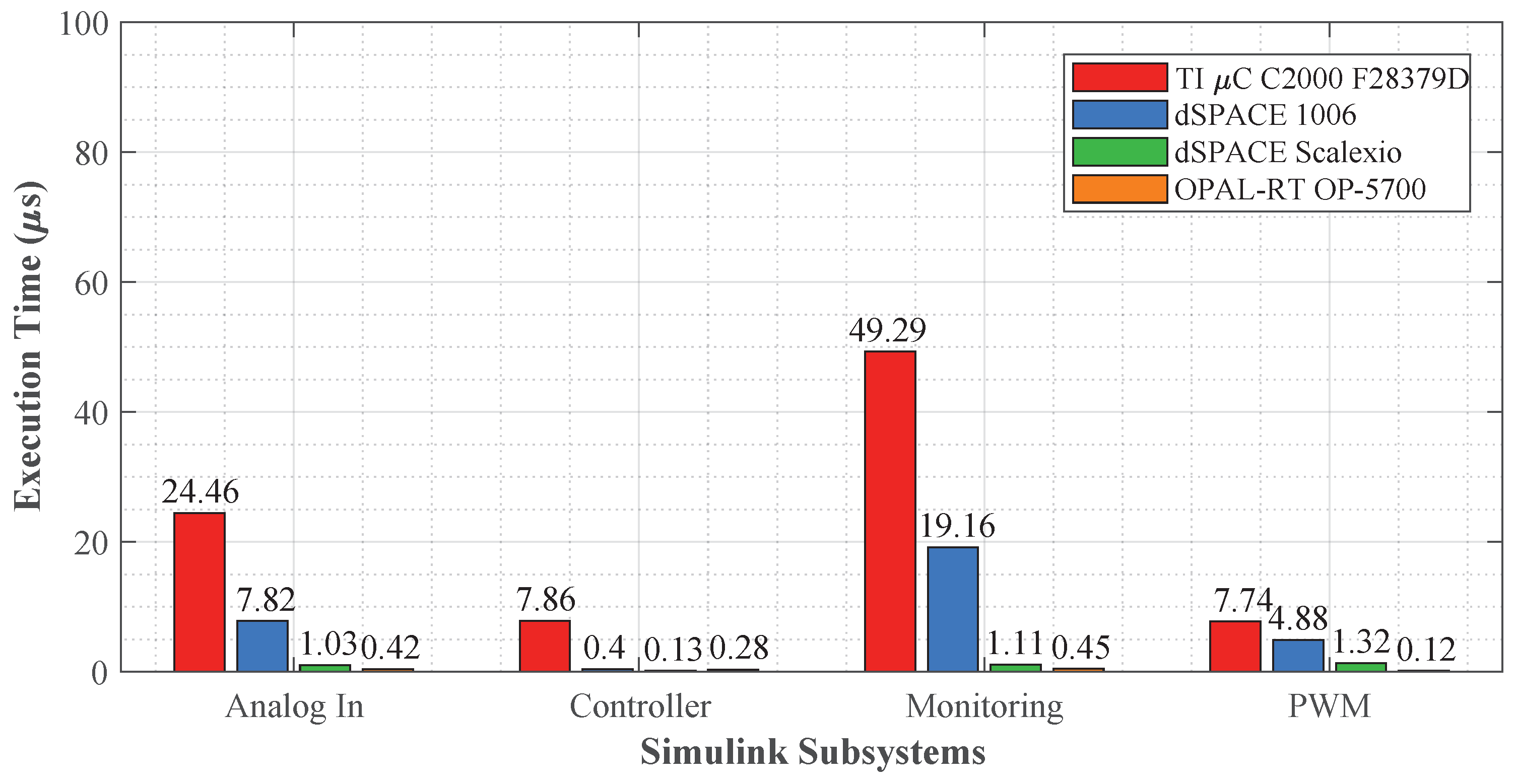
6.2.2. PI () Controller
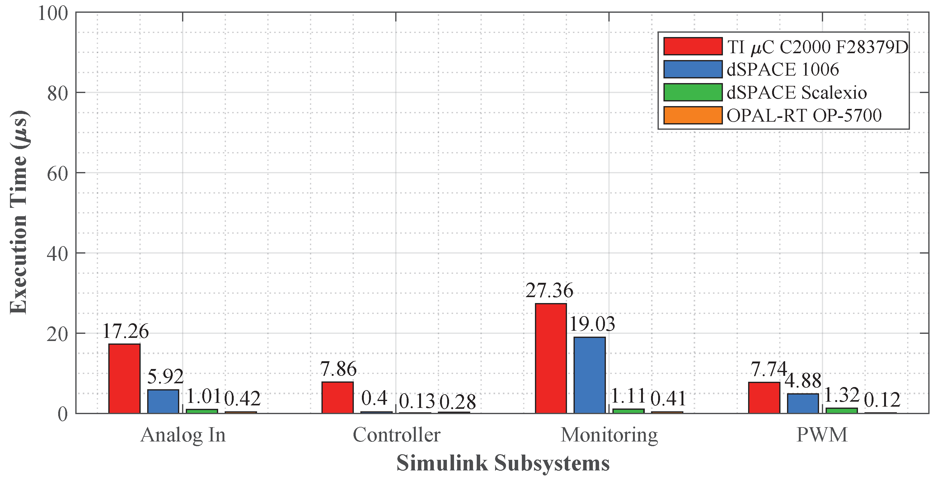
6.2.3. LQI () Controller
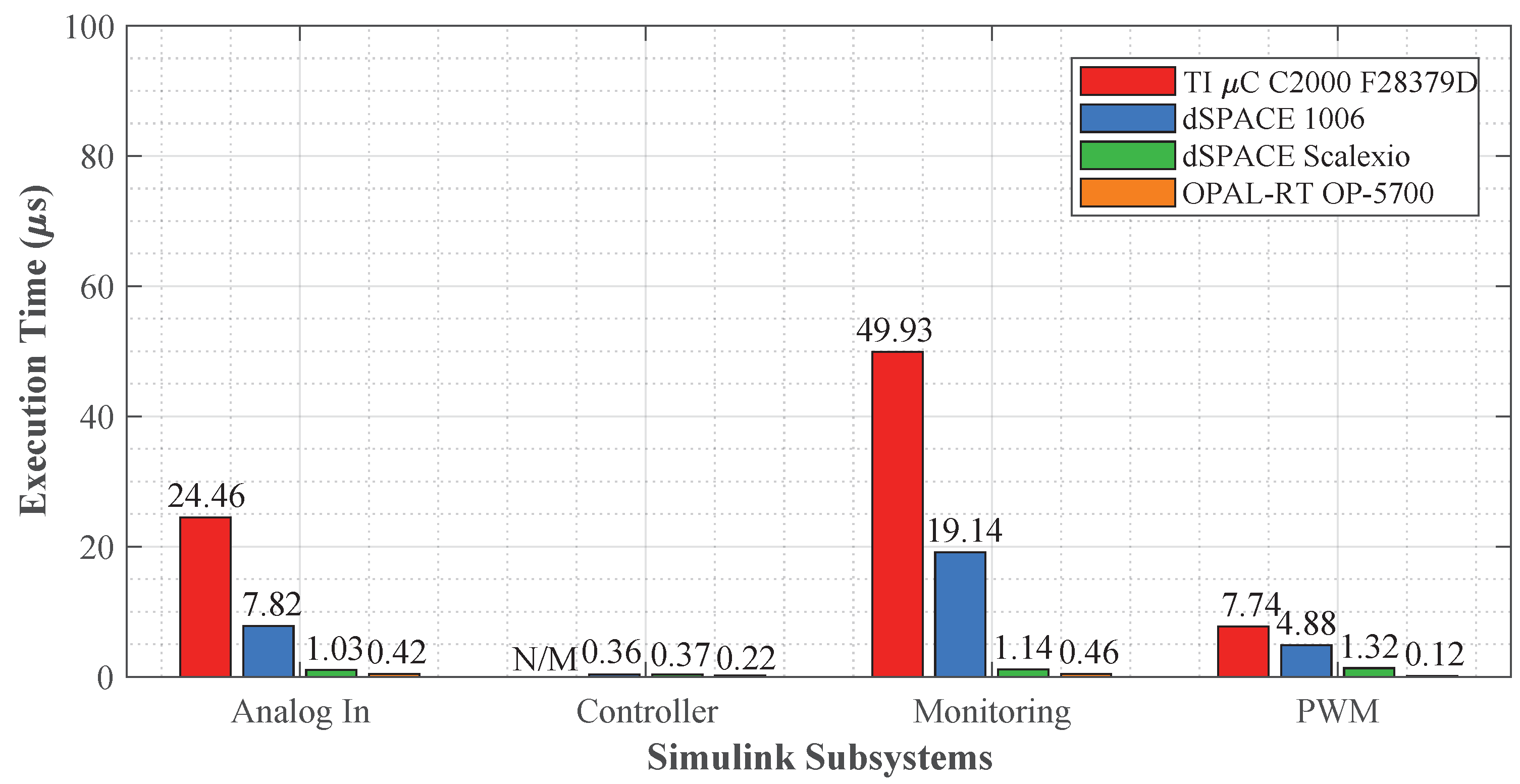
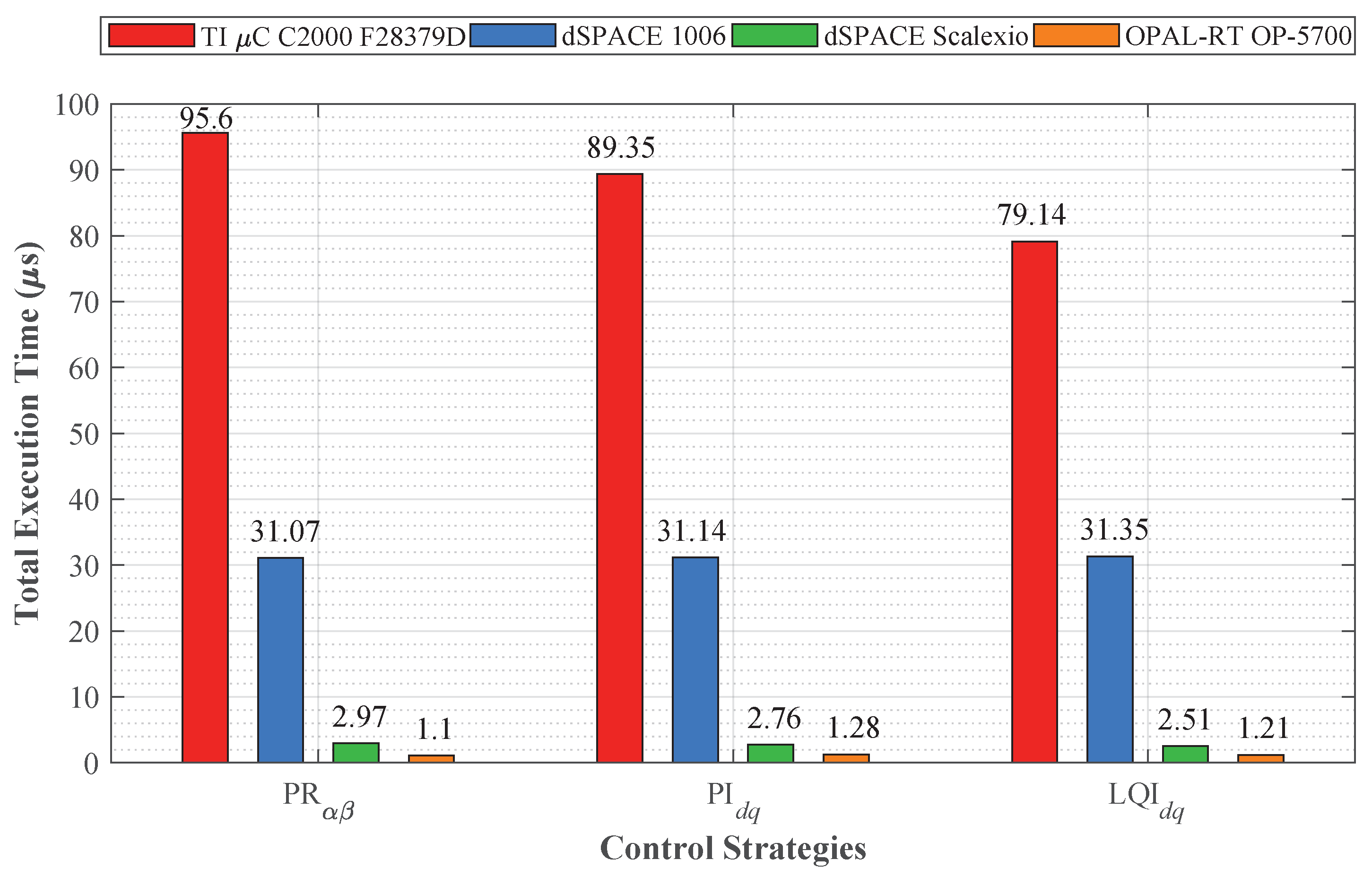
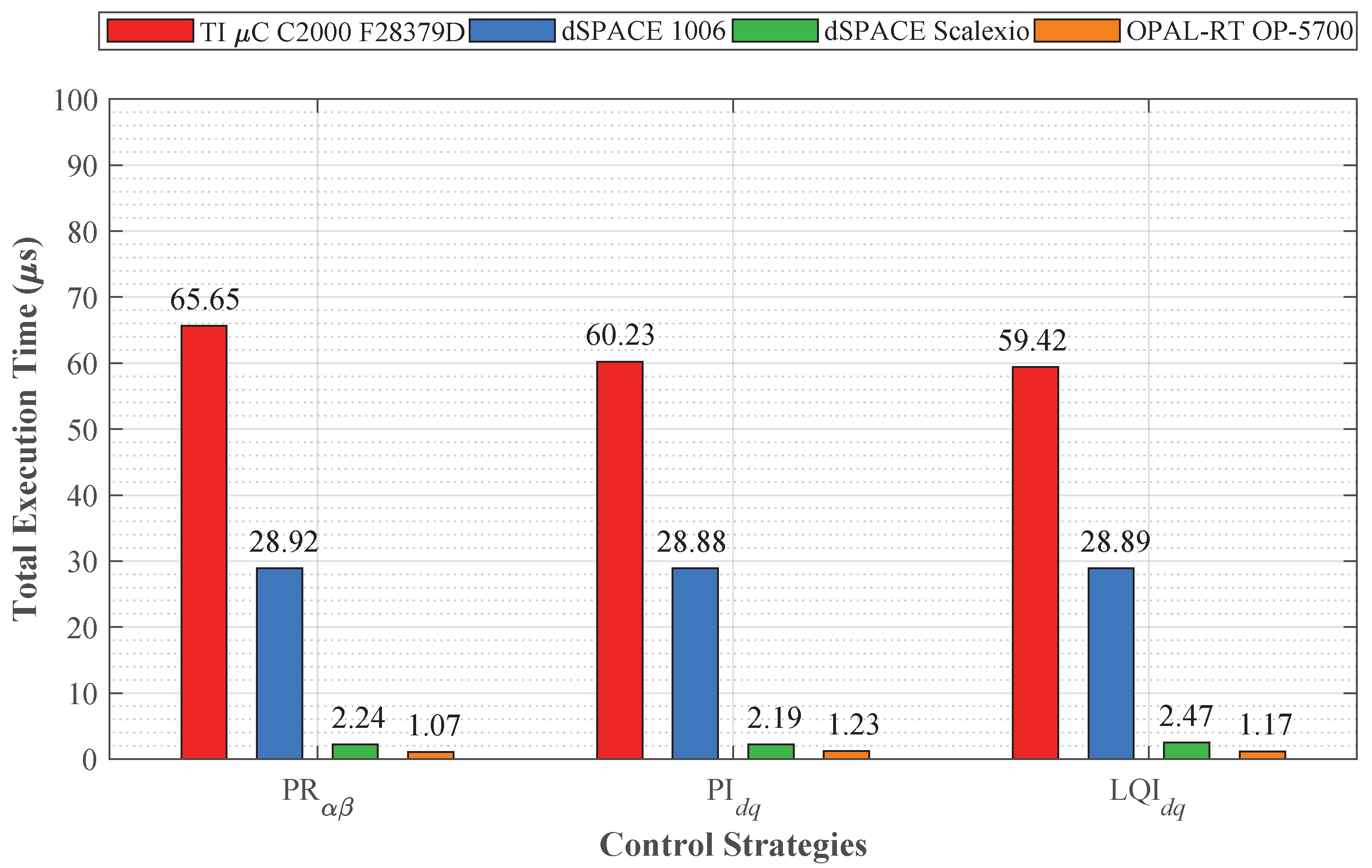
6.2.4. Total Computation Time Profiles
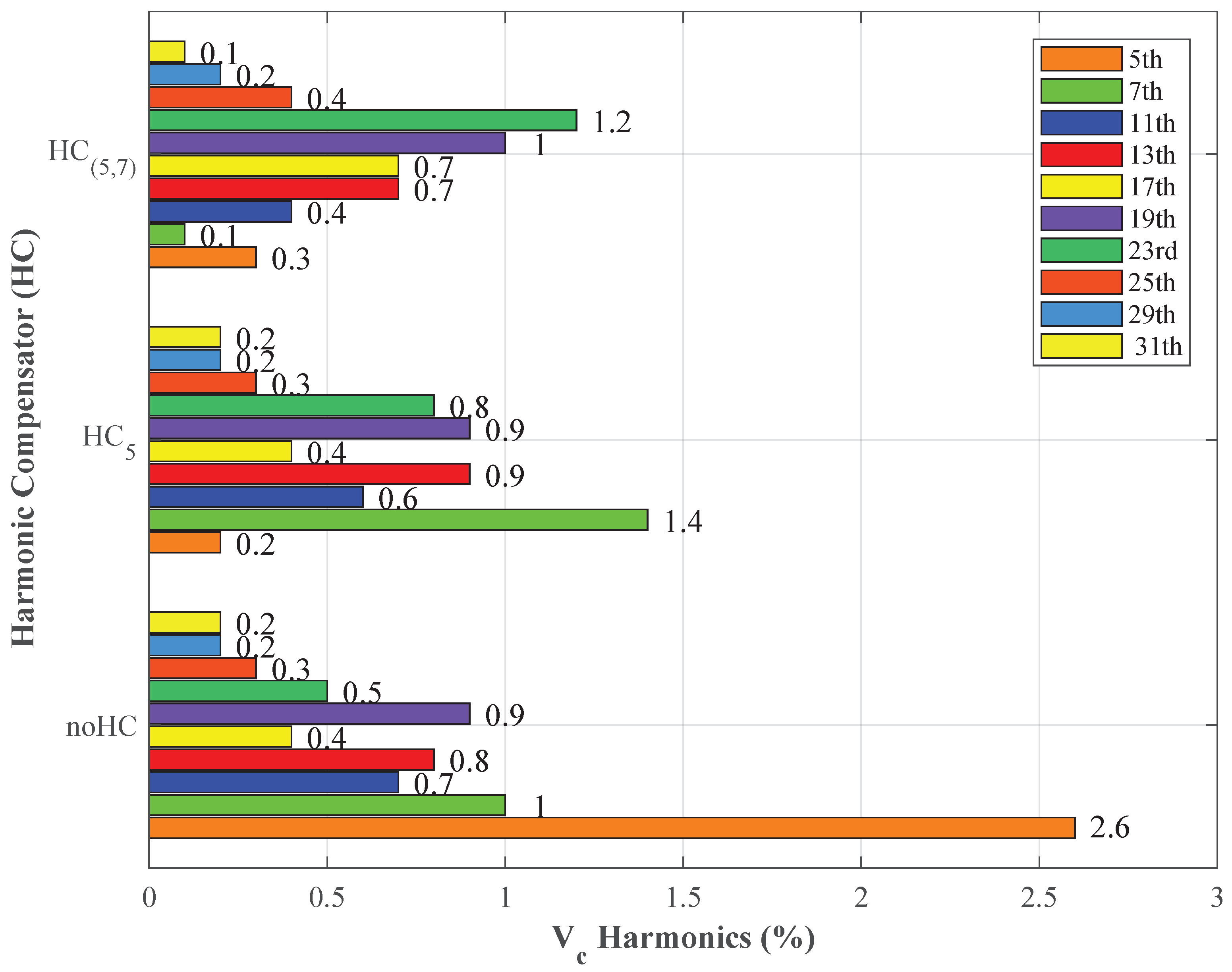
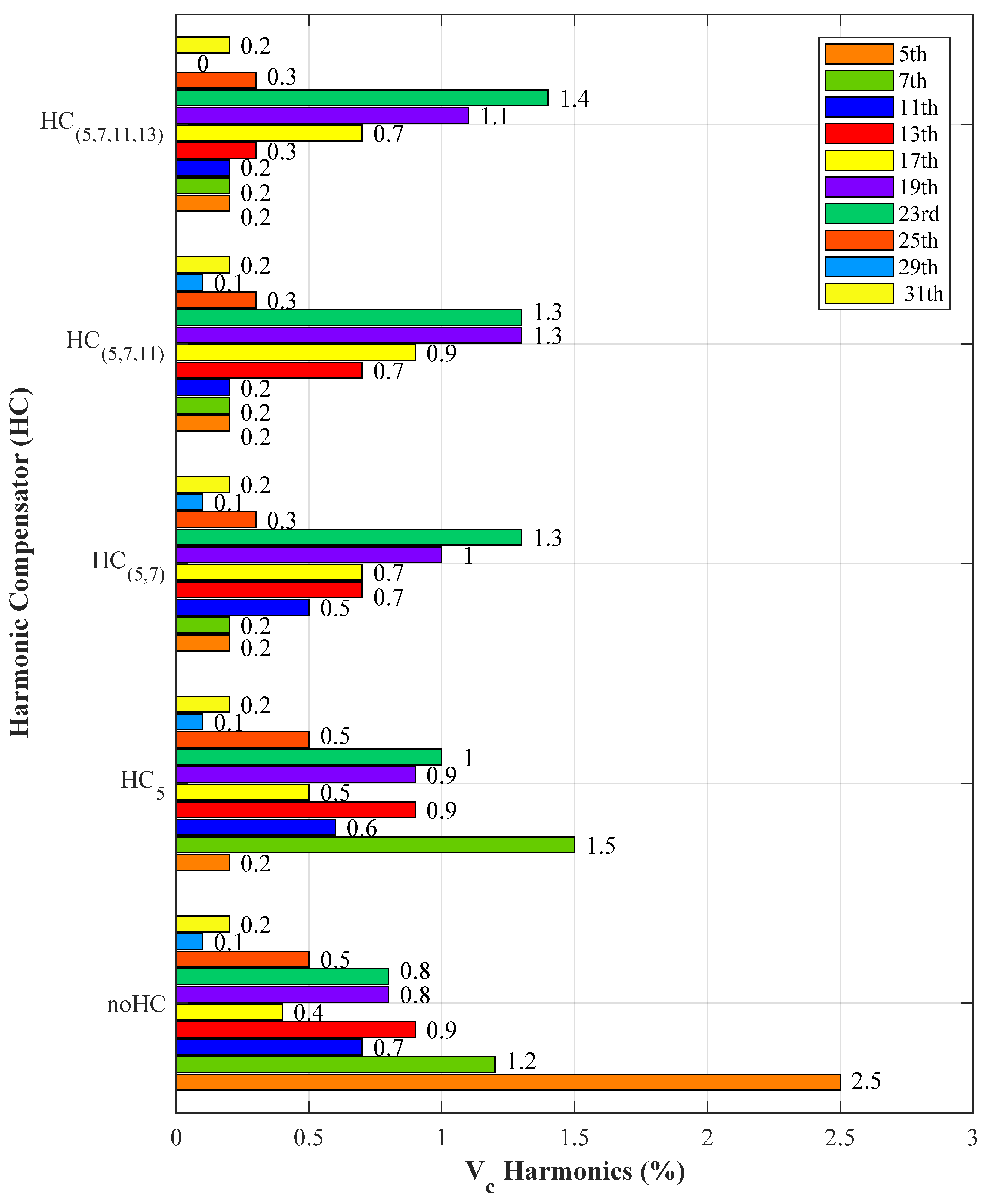
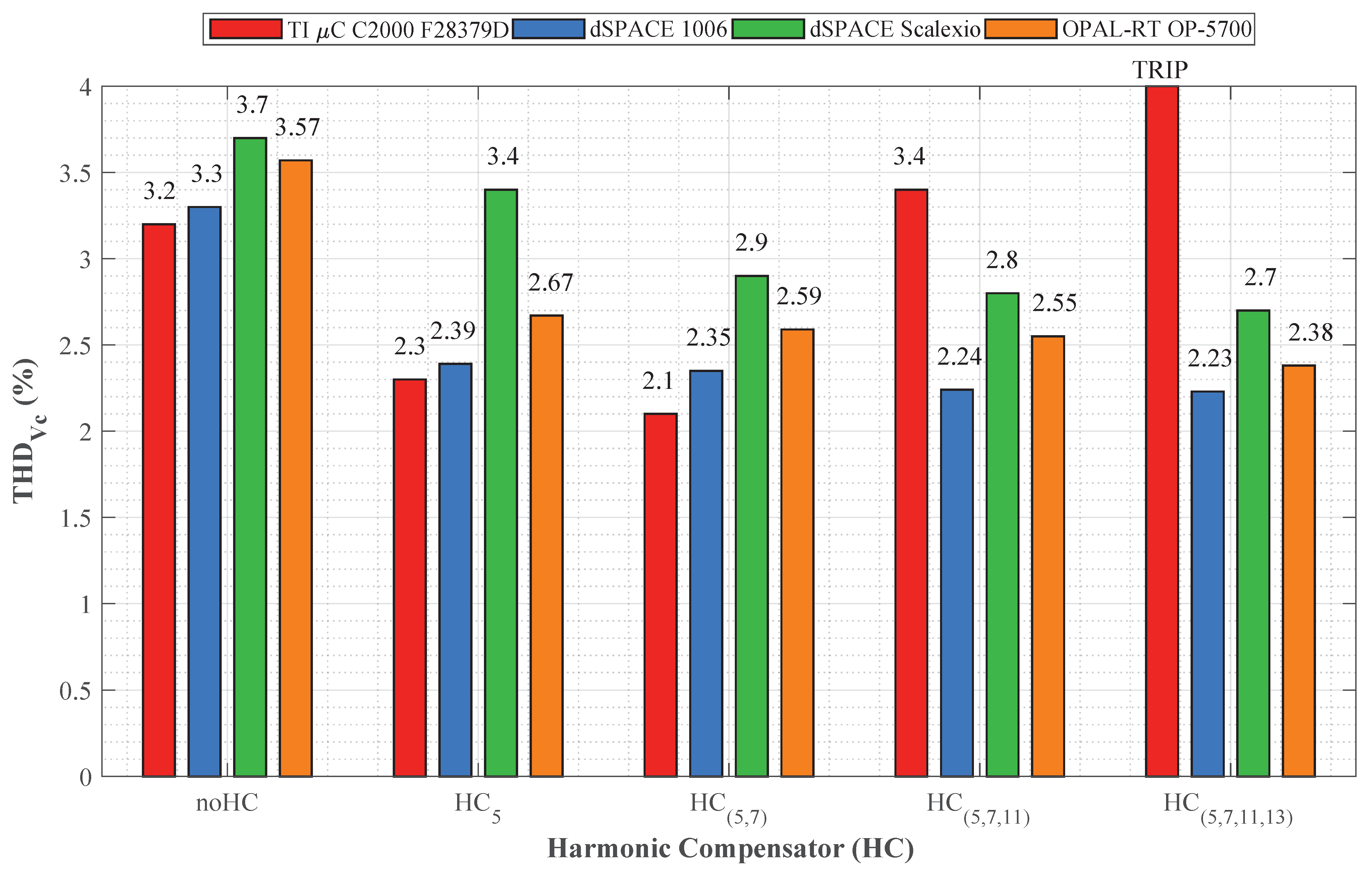
6.3. Scenario II: Harmonics Compensator with Voltage Harmonics Controller
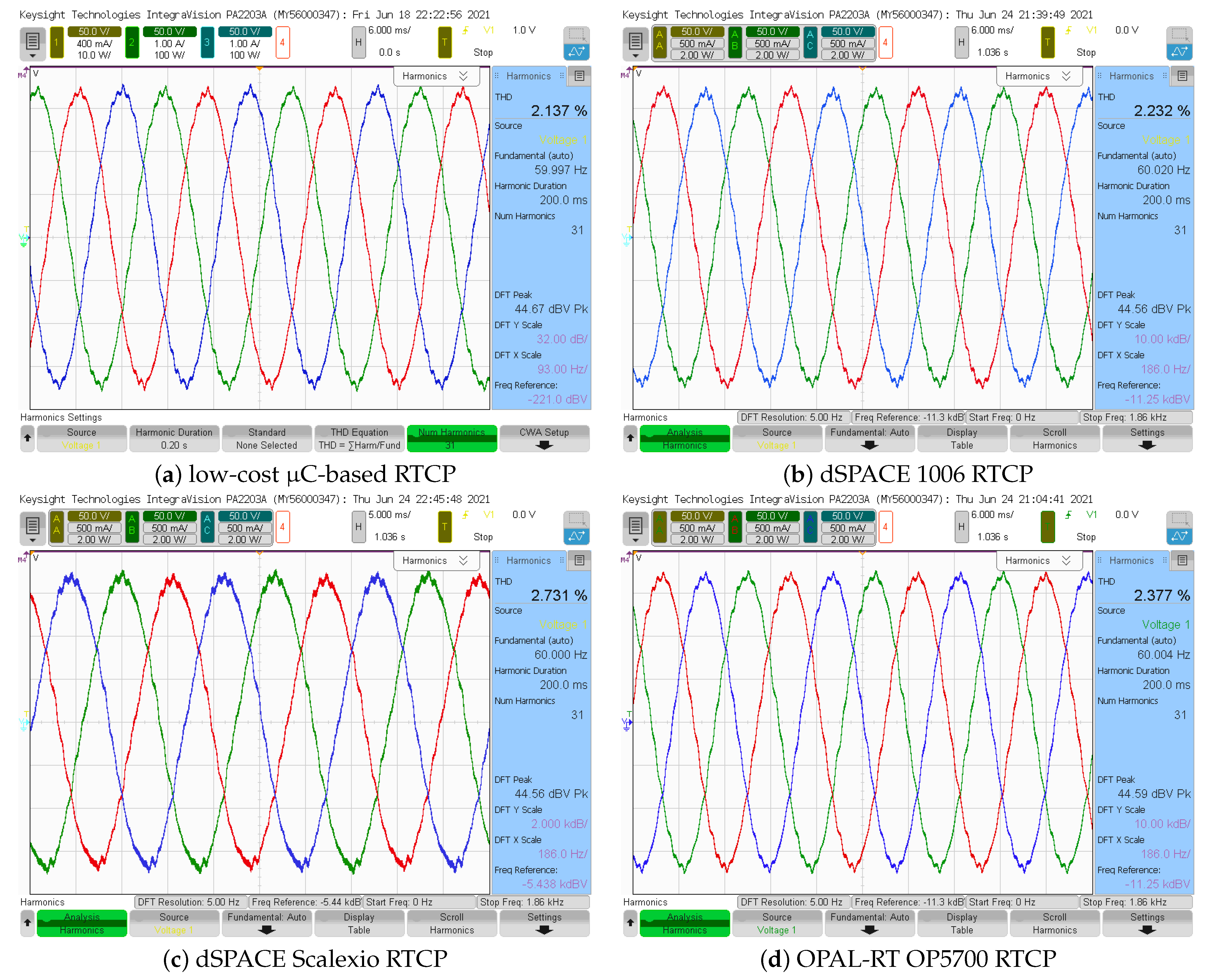
6.3.1. Low-Cost C-Based RTCP
6.3.2. dSPACE 1006 RTCP
6.3.3. dSPACE Scalexio RTCP
6.3.4. OPAL-RT OP5700 RTCP
7. Discussion
Author Contributions
Funding
Data Availability Statement
Conflicts of Interest
References
- Rashid, M.H. Alternative Energy in Power Electronics, 1st ed.; Elsevier Inc.: Amsterdam, The Netherlands, 2014; pp. 1–363. [Google Scholar] [CrossRef]
- Corradini, L.; Maksimovic, D.; Mattavelli, P.; Zane, R. Digital Control of High-Frequency Switched-Mode Power Converters; Wiley-IEEE Press: Piscataway, NJ, USA, 2015; p. 357. [Google Scholar]
- IEEE Std. 1547-2018; Standard for Interconnection and Interoperability of Distributed Energy Resources with Associated Electric Power Systems Interfaces. IEEE Standard Association: Piscataway, NJ, USA, 2018; pp. 1–138. [CrossRef]
- Vasquez-Plaza, J.D.; Patarroyo-Montenegro, J.F.; Campo-Ossa, D.D.; Sanabria-Torres, E.A.; Lopez-Chavarro, A.F.; Andrade, F. Formal Design Methodology for Discrete Proportional-Resonant (PR) Controllers Based on Sisotool/Matlab Tool. In Proceedings of the IECON 2020 The 46th Annual Conference of the IEEE Industrial Electronics Society, Singapore, 8–21 October 2020; Volume 2020, pp. 3679–3684. [Google Scholar] [CrossRef]
- Curi Busarello, T.D.; Zeb, K.; Simões, M.G. Highly Accurate Digital Current Controllers for Single-Phase LCL-Filtered Grid-Connected Inverters. Electricity 2020, 1, 12–36. [Google Scholar] [CrossRef]
- Han, Y.; Shen, P.; Zhao, X.; Guerrero, J.M. Control Strategies for Islanded Microgrid Using Enhanced Hierarchical Control Structure with Multiple Current-Loop Damping Schemes. IEEE Trans. Smart Grid 2017, 8, 1139–1153. [Google Scholar] [CrossRef]
- Patarroyo-montenegro, J.F.; Vasquez-plaza, J.D.; Andrade, F. A State-Space Model of an Inverter-Based Microgrid for Multivariable Feedback Control Analysis and Design. Energies 2020, 13, 3279. [Google Scholar] [CrossRef]
- Lopez-Chavarro, A.F.; Patarroyo-Montenegro, J.F.; Sanabria-Torres, E.A.; Campo-Ossa, D.D.; Vasquez-Plaza, J.D.; Andrade-Rengifo, F. A Design Algorithm for Multivariable Linear Quadratic Integral Controllers in Voltage-Source Converters. In Proceedings of the IECON Proceedings (Industrial Electronics Conference), Singapore, 8–21 October; Volume 2020, pp. 4025–4030. [CrossRef]
- Valencia-Rivera, G.H.; Merchan-Villalba, L.R.; Tapia-Tinoco, G.; Lozano-Garcia, J.M.; Ibarra-Manzano, M.A.; Avina-Cervantes, J.G. Hybrid LQR-PI control for microgrids under unbalanced linear and nonlinear loads. Mathematics 2020, 8, 1096. [Google Scholar] [CrossRef]
- Petkova, M.; Antchev, M.; Gourgoulitsov, V. Investigation of Single-Phase Inverter and Single-Phase Series Active Power Filter with Sliding Mode Control. Sliding Mode Control 2011. [Google Scholar] [CrossRef]
- Viswadev, R.; Mudlapur, A.; Ramana, V.V.; Venkatesaperumal, B.; Mishra, S. A Novel AC Current Sensorless Hysteresis Control for Grid-Tie Inverters. IEEE Trans. Circuits Syst. II Express Briefs 2020, 67, 2577–2581. [Google Scholar] [CrossRef]
- Sahoo, S.K.; Sinha, A.K.; Kishore, N.K. Control Techniques in AC, DC, and Hybrid AC-DC Microgrid: A Review. IEEE J. Emerg. Sel. Top. Power Electron. 2018, 6, 738–759. [Google Scholar] [CrossRef]
- Mehta, S. A comprehensive review on control techniques for stability improvement in microgrids. Int. Trans. Electr. Energy Syst. 2021, 31, e12822. [Google Scholar] [CrossRef]
- Rosso, R.; Member, S.; Wang, X.; Member, S. Grid-Forming Converters: Control Approaches, Grid-Synchronization, and Future Trends—A Review. Ind. Appl. 2021, 2, 93–109. [Google Scholar] [CrossRef]
- Ansari, S.; Chandel, A.; Tariq, M. A Comprehensive Review on Power Converters Control and Control Strategies of AC/DC Microgrid. IEEE Access 2021, 9, 17998–18015. [Google Scholar] [CrossRef]
- Gao, F.; Kang, R.; Cao, J.; Yang, T. Primary and secondary control in DC microgrids: A review. J. Mod. Power Syst. Clean Energy 2019, 7, 227–242. [Google Scholar] [CrossRef]
- Luo, F.L.; Ye, H.; Rashid, M.H.M.H. Digital Power Electronics and Applications; Elsevier Academic: Amsterdam, The Netherlands, 2005; p. 408. [Google Scholar]
- Buccella, C.; Cecati, C.; Latafat, H. Digital control of power converters—A survey. IEEE Trans. Ind. Inform. 2012, 8, 437–447. [Google Scholar] [CrossRef]
- Liu, Y.F.; Sen, P. Digital control of switching power converters. In Proceedings of 2005 IEEE Conference on Control Applications, CCA 2005, Toronto, ON, Canada, 29–31 August 2005; pp. 635–640. [Google Scholar] [CrossRef]
- Maksimovic, D.; Zane, R.; Erickson, R. Impact of digital control in power electronics. In Proceedings of the Intemational Symposium on Power Semiconductor Devices &ICs, Orlando, FL, USA, 18–22 May 2008; pp. 13–22. [Google Scholar] [CrossRef]
- Yousefzadeh, V. Advances in digital power control. In Proceedings of the INTELEC, International Telecommunications Energy Conference, Orlando, FL, USA, 6–10 June 2010. [Google Scholar] [CrossRef]
- dSPACE Systems. Products—dSPACE; dSPACE Systems: Paderborn, Germany, 2021. [Google Scholar]
- OPAL-RT Technologies. HIL Testing |FPGA Technology|RCP Technologies; OPAL-RT Technologies: Montréal, QC, Canada, 2021. [Google Scholar]
- Typhoon HIL. HIL Hardware—Typhoon HIL; Typhoon HIL: Somerville, MA, USA, 2021. [Google Scholar]
- RTDS Technologies. Power Electronics HIL—RTDS Technologies; RTDS Technologies: Winnipeg, MB, Canada, 2021. [Google Scholar]
- Plexim: Electrical Engineering Software; RT Box|Plexim: Zürich, Switzerland, 2021.
- Imperix—Rapid Control Prototyping Solutions for Power Electronics. Power Electronic Controllers—Programmable Digital Controllers. 2021. Available online: https://imperix.com/products/power-electronic-controllers/ (accessed on 8 September 2022).
- PED-Board. PED-Board|Just Add Power. Available online: https://www.ped-board.com/ (accessed on 8 September 2022).
- Bastos, R.F.; Fuzato, G.H.; Aguiar, C.R.; Neves, R.V.; Machado, R.Q. Model, design and implementation of a low-cost HIL for power converter and microgrid emulation using DSP. IET Power Electron. 2019, 12, 3833–3841. [Google Scholar] [CrossRef]
- Vasquez Plaza, J.D.; Patarroyo-Montenegro, J.F.; Andrade, F. Development and Implementation of a Low-Cost Research Platform for Control Applications for Inverter-Based Generators. In Proceedings of the 2020 22nd European Conference on Power Electronics and Applications, EPE 2020 ECCE Europe, Lyon, France, 7–11 September 2020; pp. 1–9. [Google Scholar] [CrossRef]
- Aravena, J.; Carrasco, D.; Diaz, M.; Uriarte, M.; Rojas, F.; Cardenas, R.; Travieso, J.C. Design and implementation of a low-cost real-time control platform for power electronics applications. Energies 2020, 13, 1527. [Google Scholar] [CrossRef]
- Texas Instruments Inc. C2000™ Real-Time Microcontrollers; Texas Instruments Inc.: Dallas, TX, USA, 2021. [Google Scholar]
- Yuan, S.; Shen, Z. The design of Matlab-DSP development environment for control system. In Proceedings of the 2012 3rd International Conference on Digital Manufacturing and Automation, ICDMA 2012, Guilin, China, 31 July–2 August 2012; pp. 903–906. [Google Scholar] [CrossRef]
- Patil, P.H.; Kapse, K. Transition from Simulink to MATLAB in real-time digital signal processing. In Proceedings of the 2015 International Conference on Electrical, Electronics, Signals, Communication and Optimization (EESCO), Visakhapatnam, India, 24–25 January 2015; Volume 21. [Google Scholar] [CrossRef]
- Hýl, R.; Wagnerová, R. Fast development of controllers with Simulink Coder. In Proceedings of the 2017 18th International Carpathian Control Conference, ICCC 2017, Sinaia, Romania, 28–31 May 2017; pp. 406–411. [Google Scholar] [CrossRef]
- Dos Santos, B.; Araujo, R.E.; Varajao, D.; Pinto, C. Rapid Prototyping Framework for real-time control of power electronic converters using simulink. In Proceedings of the IECON Proceedings (Industrial Electronics Conference), Vienna, Austria, 10–13 November 2013; pp. 2303–2308. [Google Scholar] [CrossRef]
- Kyslan, K.; Lacko, M.; Ferková, Ž.; Záskalický, P. V/f control of five phase induction machine implemented on DSP using simulink coder. In Proceedings of the 13th International Conference ELEKTRO 2020, ELEKTRO 2020-Proceedings, Taormina, Italy, 25–28 May 2020; Volume 2020, pp. 1–6. [Google Scholar] [CrossRef]
- Grepl, R. Real-time control prototyping in MATLAB/simulink: Review of tools for research and education in mechatronics. In Proceedings of the 2011 IEEE International Conference on Mechatronics, ICM 2011-Proceedings, Istanbul, Turkey, 3–15 April 2011; pp. 881–886. [Google Scholar] [CrossRef]
- Omar Faruque, M.D.; Strasser, T.; Lauss, G.; Jalili-Marandi, V.; Forsyth, P.; Dufour, C.; Dinavahi, V.; Monti, A.; Kotsampopoulos, P.; Martinez, J.A.; et al. Real-Time Simulation Technologies for Power Systems Design, Testing, and Analysis. IEEE Power Energy Technol. Syst. J. 2015, 2, 63–73. [Google Scholar] [CrossRef]
- Ruiz, G.E.; Munoz, N.; Cano, J.B. Design methodologies and programmable devices used in power electronic converters—A survey. In Proceedings of the 2015 IEEE Workshop on Power Electronics and Power Quality Applications, PEPQA 2015-Proceedings, Bogotá, Colombia, 2–4 June 2015; pp. 4–9. [Google Scholar] [CrossRef]
- Lee, Y.S.; Jo, B.; Han, S. A Light-Weight Rapid Control Prototyping System Based on Open Source Hardware. IEEE Access 2017, 5, 11118–11130. [Google Scholar] [CrossRef]
- Li, F.; Wang, Y.; Wu, F.; Huang, Y.; Liu, Y.; Zhang, X.; Ma, M. Review of Real-time Simulation of Power Electronics. J. Mod. Power Syst. Clean Energy 2020, 8, 796–808. [Google Scholar] [CrossRef]
- Lamberský, V.; Vejlupek, J. Benchmarking the Performance of A DSPIC Controller Programed with Automatically Generated Code. Tech. Comput. Prague 2011, 75. [Google Scholar]
- Březina, T.; Jabłoński, R. Mechatronics 2013: Recent Technological and Scientific Advances; Springer International Publishing: Berlin/Heidelberg, Germany, 2013; pp. 669–675. [Google Scholar]
- Dufour, C.; Ould Bachir, T.; Grégoire, L.A.; Bélanger, J. Real-time simulation of power electronic systems and devices. In Dynamics and Control of Switched Electronic Systems; Springer: London, UK, 2012; pp. 451–487. [Google Scholar] [CrossRef]
- The MathWorks Inc. Simulink Coder; The MathWorks Inc.: Natick, MA, USA, 2021. [Google Scholar]
- MathWorks Inc. What is Simulink Coder?—MATLAB & Simulink; MathWorks Inc.: Natick, MA, USA, 2021. [Google Scholar]
- The MathWorks Inc. Simscape; The MathWorks Inc.: Natick, MA, USA, 2021. [Google Scholar]
- Texas Instruments Inc. C2000-CGT; Texas Instruments Inc.: Dallas, TX, USA, 2021. [Google Scholar]
- Opal-RT Technologies Inc. RT-LAB Installion Guide; Opal-RT Technologies Inc.: Montréal, QC, Canada, 2021. [Google Scholar]
- DSPACE GmbH. Translating C Code into dSPACE Platforms; DSPACE GmbH: Paderborn, Germany, 2016. [Google Scholar]
- Sanabria-Torres, E.A.; Rengifo, F.A.; Patarroyo-Montenegro, J.F.; Vasquez-Plaza, J.D.; Lopez-Chavarro, A.F.; Campo-Ossa, D.D. Design of Proportional-Resonant Controllers for Voltage-Source Converters using State-Space Model. In Proceedings of the IECON 2021—47th Annual Conference of the IEEE Industrial Electronics Society, Toronto, ON, Canada, 13–16 October 2021; pp. 1–6. [Google Scholar] [CrossRef]
- Vasquez, J.C.; Guerrero, J.M.; Savaghebi, M.; Eloy-Garcia, J.; Teodorescu, R. Modeling, Analysis, and Design of Stationary-Reference-Frame Droop-Controlled Parallel Three-Phase Voltage Source Inverters. IEEE Trans. Ind. Electron. 2013, 60, 1271–1280. [Google Scholar] [CrossRef]
- Hao, M.; Zhen, X. A control strategy for voltage source inverter adapted to multi—Mode operation in microgrid. In Proceedings of the 2017 36th Chinese Control Conference, Dalian, China, 26–28 July 2017; pp. 9163–9168. [Google Scholar]
- Pogaku, N.; Prodanovic, M.; Green, T.C. Modeling, analysis and testing of autonomous operation of an inverter-based microgrid. IEEE Trans. Power Electron. 2007, 22, 613–625. [Google Scholar] [CrossRef]
- Patarroyo-Montenegro, J.F.; Andrade, F.; Guerrero, J.M.; Vasquez, J.C. A Linear Quadratic Regulator With Optimal Reference Tracking for Three-Phase Inverter-Based Islanded Microgrids. IEEE Trans. Power Electron. 2021, 36, 7112–7122. [Google Scholar] [CrossRef]
- Patarroyo-Montenegro, J.F.; Vasquez-Plaza, J.D.; Andrade, F.; Fan, L. An Optimal Power Control Strategy for Grid-Following Inverters in a Synchronous Frame. Appl. Sci. 2020, 10, 6730. [Google Scholar] [CrossRef]
- Lewis, F.L.; Vrabie, D.L.; Syrmos, V.L. Optimal Control; John Wiley & Sons, Inc.: Hoboken, NJ, USA, 2012. [Google Scholar] [CrossRef]
- Huerta, F.; Pizarro, D.; Cóbreces, S.; Rodríguez, F.J.; Girón, C.; Rodríguez, A. LQG servo controller for the current control of LCL grid-connected Voltage-Source Converters. IEEE Trans. Ind. Electron. 2012, 59, 4272–4284. [Google Scholar] [CrossRef]
- Mathworks Inc. Real-Time Code Execution Profiling—MATLAB & Simulink Example; Mathworks Inc.: Natick, MA, USA, 2021. [Google Scholar]
- MathWorks Inc. Overview of Creating a Model and Generating Executable for C2000 Processors—MATLAB & Simulink. Available online: https://ww2.mathworks.cn/help/supportpkg/texasinstrumentsc2000/modeling.html (accessed on 8 September 2022).
- dSPACE. dSPACE Profiler; dSPACE: Paderborn, Germany, 2022. [Google Scholar]
- Monitoring View—RT-LAB Documentation—Wiki OPAL-RT. Available online: https://wiki.opal-rt.com/display/RD/RT-LAB+Documentation (accessed on 8 September 2022).
- Patarroyo-Montenegro, J.F.; Salazar-Duque, J.E.; Alzate-Drada, S.I.; Vasquez-Plaza, J.D.; Andrade, F. An AC Microgrid Testbed for Power Electronics Courses in the University of Puerto Rico at Mayagüez. In Proceedings of the 2018 IEEE ANDESCON, ANDESCON 2018-Conference Proceedings, Cali, Colombia, 22–24 August 2018; pp. 1–6. [Google Scholar]
- Teodorescu, R.; Liserre, M.; Pedro, R. Grid Converters for Photovoltaic and Wind Power Systems; John Wiley & Sons: Hoboken, NJ, USA, 2011. [Google Scholar]


| RTCP Brand/Model | Features | Computational Engine | Price | Software | ||||||
|---|---|---|---|---|---|---|---|---|---|---|
| DI | DO | ADC | PWM | |||||||
| No. | No. | No. | Resolution | Conv. Time | No. | Max. Freq. | ||||
| Based in TI C C2000 F28379D | 169 Shared | 169 Shared | 16 | 16/12 bits | 0.91 s | 24 Shared | 100 MHz | Dual Core 32-bit CPUs 200MHz | $ | Free |
| dSPACE 1006 | 96 Shared | 96 Shared | 48 | 16 bits | 0.80 s | 16 | 2 MHz | Quad-core AMD Opteron, 2.8 GHz | $$ | Licensed |
| dSPACE Scalexio | 96 Shared | 96 Shared | 48 | 16 bits | 0.25 s | 96 Shared | 0.5 MHz | Quad-core Intel i7-6820EQ, 2.8 GHz | $$$ | Licensed |
| OPAL-RT OP5700 | 32 | 32 | 16 | 16 bits | 1 s | 32 Shared | 0.5 MHz | Xilinx Virtex-7 FPGA Intel Xeon E5 8 Cores 3.2 GHz | $$$$$ | Licensed |
| Blocks | LQI () | PR () | PI () |
|---|---|---|---|
| PWM | x | x | x |
| Duty Generator | x | x | x |
| DI | x | x | x |
| DO | x | x | x |
| ADC | x | x | x |
| Voltage Reference Generator | x | x | x |
| Integrator | x | x | x |
| ABC/ Conversion | x | x | |
| /ABC Conversion | x | x | |
| ABC/ Conversion | x | ||
| /ABC Conversion | x | ||
| RMS | x | x | x |
| THD | x | x | x |
| Matrix Product | x |
| Parameter | Value | ||
|---|---|---|---|
| DC/AC SPC | Switching frequency, | 10 kHz | |
| Sampling Period, | 100 s | ||
| Nominal frequency, | 60 Hz | ||
| Rated voltage, V | 120 V | ||
| Filter capacitance, | 8.8 F | ||
| Filter internal inductance, | 1.8 mH | ||
| Filter output inductance, | 1.8 mH | ||
| DC link voltage, | 350 V | ||
| Control Strategy | PI () | 1.5, 100, 0.1, 200 | |
| PR () | 1.5, 100, 0.1, 200 | ||
| LQI () | |||
| Non-Linear Load | Capacitance, | 100 F | |
| Inductance, | 2 mH | ||
| Resistance, | 250 | ||
| Harmonics Compensator () | Parameter | Value | |
|---|---|---|---|
| Fundamental () | 1.5, 100, 0.1, 200 | ||
| Fifth Harmonic () | 80 | ||
| Seventh Harmonic () | 95 | ||
| Eleventh Harmonic () | 65 | ||
| Thirteenth Harmonic () | 105 | ||
| Seventeenth Harmonic () | 100 | ||
Publisher’s Note: MDPI stays neutral with regard to jurisdictional claims in published maps and institutional affiliations. |
© 2022 by the authors. Licensee MDPI, Basel, Switzerland. This article is an open access article distributed under the terms and conditions of the Creative Commons Attribution (CC BY) license (https://creativecommons.org/licenses/by/4.0/).
Share and Cite
Vasquez-Plaza, J.D.; Lopez-Chavarro, A.F.; Sanabria-Torres, E.A.; Patarroyo-Montenegro, J.F.; Andrade, F. Benchmarking Real-Time Control Platforms Using a Matlab/Simulink Coder with Applications in the Control of DC/AC Switched Power Converters. Energies 2022, 15, 6940. https://doi.org/10.3390/en15196940
Vasquez-Plaza JD, Lopez-Chavarro AF, Sanabria-Torres EA, Patarroyo-Montenegro JF, Andrade F. Benchmarking Real-Time Control Platforms Using a Matlab/Simulink Coder with Applications in the Control of DC/AC Switched Power Converters. Energies. 2022; 15(19):6940. https://doi.org/10.3390/en15196940
Chicago/Turabian StyleVasquez-Plaza, Jesus D., Andres F. Lopez-Chavarro, Enrique A. Sanabria-Torres, Juan F. Patarroyo-Montenegro, and Fabio Andrade. 2022. "Benchmarking Real-Time Control Platforms Using a Matlab/Simulink Coder with Applications in the Control of DC/AC Switched Power Converters" Energies 15, no. 19: 6940. https://doi.org/10.3390/en15196940
APA StyleVasquez-Plaza, J. D., Lopez-Chavarro, A. F., Sanabria-Torres, E. A., Patarroyo-Montenegro, J. F., & Andrade, F. (2022). Benchmarking Real-Time Control Platforms Using a Matlab/Simulink Coder with Applications in the Control of DC/AC Switched Power Converters. Energies, 15(19), 6940. https://doi.org/10.3390/en15196940