A Novel Hybrid Machine Learning Model for Wind Speed Probabilistic Forecasting

Abstract

Accurately capturing wind speed fluctuations and quantifying the uncertainties has important implications for energy planning and management. This paper proposes a novel hybrid machine learning model to solve the problem of probabilistic prediction of wind speed. The model couples the light gradient boosting machine (LGB) model with the Gaussian process regression (GPR) model, where the LGB model can provide high-precision deterministic wind speed prediction results, and the GPR model can provide reliable probabilistic prediction results. The proposed model was applied to predict wind speeds for a real wind farm in the United States. The eight contrasting models are compared in terms of deterministic prediction and probabilistic prediction, respectively. The experimental results show that the LGB-GPR model improves the point forecast accuracy (RMSE) by up to 20.0% and improves the probabilistic forecast reliability (CRPS) by up to 21.5% compared to a single GPR model. This research is of great significance for improving the reliability of wind speed, probabilistic predictions, and the sustainable development of new energy.

1. Introduction

With the rapid development of science and technology industries, fossil fuel energy has been consumed in large quantities, which has led to a series of problems, such as the greenhouse effect, resource shortage, and environmental pollution [1,2]. To alleviate and improve the existing energy crisis and resource scheduling problems, people focus on the development of renewable and nonpolluting new energies. Wind energy is one of the most common sources of energy in nature and accounts for a large proportion of the development of renewable energy [3,4]. Wind-speed prediction is also important for the wind-resistant design of bridges [5] and railway infrastructure [6]. However, the nonstationary, nonlinearity, and intermittency of wind-energy resources will lead to uneven wind-power output of wind turbines, which hinders grid security maintenance, power quality, and power scheduling and planning [7,8]. For wind-power generation systems, the difficulty and cost of storing electricity is much higher than generating electricity, and most generators are in the form of direct power generation [9,10]. This is very different from traditional regulated energy sources, such as hydroelectricity [11,12]. Another difficulty with wind power generation is the integration of wind power into the grid [13]. A large number of intermittent energy grids will lead to unbalanced and unstable power-frequency regulation ranges and peak values during the peak period of electricity consumption [14]. Therefore, finding an accurate and robust wind-speed prediction method has always been an important research direction for related scholars.

Wind-speed prediction methods can be generally divided into two categories: physical methods and statistical methods [15]. Physical methods build predictive models through complex physical laws and meteorological boundary information [16]. In general, physical methods have a more stable effect on long-term wind-speed predictions. Numerical weather prediction (NWP) [17] is the most common physical method. For example, Yamaguchi et al. [18] proposed a wind-speed forecasting method based on an autoregressive model. The experimental results showed that the use of high-level resolution numerical weather forecasting can effectively improve wind-speed forecasting accuracy. Zhao et al. [19] developed a selective ensemble system based on the NWP. The experimental results showed that the proposed method can obtain accurate wind-speed prediction results by automatically culling underperforming members. Chen et al. [20] employed the Gaussian process and the NWP model to predict next-day wind power. The results showed that the accuracy of the prediction of the proposed model is better than that of the comparison model. However, the use of physical models requires complex physical variables and time-consuming solution times.

Unlike physical methods, statistical methods do not require complex physical variables, and only need historical meteorological data to build predictive models [21,22]. In general, statistical methods have better performance in short-term wind-speed prediction. The widely used traditional statistical methods include stochastic models [23], autoregressive models (AR) [24,25], and Markov chains [26]. Pablo et al. [27] proposed a wind-speed model based on the Ornstein–Uhlenbeck process and applied the model to predict the average wind speed of a wind field in Mexico. Karakus et al. [28] proposed a wind-speed prediction model based on the polynomial AR model for the forecast of the previous day. The experimental results showed that this model outperforms all other models in both speed prediction and power prediction. Tang et al. [29] improved the traditional Markov chain and proposed a new state classification step and wind-speed simulation method. The results showed that this proposed model outperforms traditional modeling methods. However, traditional statistical methods are mostly based on the assumption of stationarity and cannot effectively extract nonstationary features in wind-speed series.

The advent of machine learning models solves this dilemma. Common machine learning models are K-nearest neighbor (KNN) [30], random forest (RF) [31], artificial neural networks (ANN) [32], support vector regression (SVR) [33,34], etc. For example, Zhang et al. [35] developed a short-term wind-speed forecasting model, GA-ANN. The results of the paper showed that the model can significantly improve the accuracy of short-term wind-speed predictions. Ren et al. [36] developed a new wind-speed prediction model by combining SVR and empirical mode decomposition, and the results showed that the proposed model outperforms several contrast methods in terms of accuracy or computational complexity. Wang et al. [37] proposed an RF-based wind-speed forecasting method. The results showed that the proposed method can effectively improve the training efficiency and the accuracy of wind-speed predictions. Owing to the characteristics of the machine learning model, the nonstationary features in the wind-speed sequence were effectively extracted, and the accuracy of wind-speed prediction was improved to a certain extent.

With the deepening of research, relevant scholars have found that the prediction performance of a single model always has certain limitations [38,39]. Combining multiple models can obtain better prediction results. Therefore, there is a growing trend to combine different individual models. For instance, Cadenas et al. [40] developed an ensemble model combining the ANN and the autoregressive integrated moving average (ARIMA) model. The results showed that the generalization ability of the ensemble model is better than that of the ARIMA and ANN models alone. In [41], a hybrid model based on modal decomposition and an extreme learning machine is proposed for short-term wind-speed predictions, and it is found that the proposed prediction model can effectively improve the reliability of multistep wind-speed predictions. Wang et al. [42] proposed a hybrid model combining the AdaBoost with the extreme learning machine (ELM) algorithm and verified that the proposed model is a method with more potential than traditional methods.

However, most of the existing studies focus on improving the accuracy of wind-speed predictions, ignoring the quantification of uncertainty in wind-speed series. Accurately capturing the probability distribution of wind-speed sequences can provide more abundant decision-making information for dispatchers, which is conducive to efficient planning and rational allocation of resources. Therefore, it is necessary to carry out wind-speed probability prediction research. This paper developed a novel hybrid model, LGB-GPR, which combines light gradient boosting machine (LGB) and Gaussian process regression (GPR) for wind-speed forecasting and quantifying forecast uncertainty. Among them, the LGB model can provide accurate wind-speed deterministic prediction results, but cannot quantify the wind-speed uncertainty. In contrast, the GPR model can quantify the uncertainty of wind speed, but its prediction accuracy is poor. The fusion of the above two models can give full play to their advantages. The innovations and main contributions of this paper are summarized as follows:

(1)

A new machine learning method named LGB is used to predict wind-speed sequences, which can provide accurate wind-speed prediction results.

(2)

A novel hybrid model combining LGB and GPR is proposed for wind-speed probability prediction.

(3)

The proposed hybrid model is applied to a real case in the United States and compared with eight contrasting models.

The rest of the paper is organized as follows: In Section 2, a brief description of LGB, GPR, and the model LGB-GPR are introduced. The evaluation metrics are given in Section 3. The data usage and experimental setup are presented in Section 4. Comparative results and discussion are presented in Section 5. At last, conclusions and future research of this study are given in Section 6.

2. Methodology

To solve the wind-speed probability prediction problem, this paper proposes a new hybrid model, LGB-GPR. In this section, we first describe the formulation and principles of the LGB model and the GPR model, respectively. Then, how to couple the LGB model and the GPR model to obtain reliable wind-speed probabilistic prediction results is described in detail.

2.1. Light Gradient Boosting Machine

Light gradient boosting machine (LGB) is an improved gradient boosting decision tree (GBDT) model proposed by Microsoft. It solves the problems of slow training speed and large memory usage of the traditional gradient boosting decision tree model in the face of large data volume and high feature dimension, and at the same time, has higher accuracy. LGB is a lifting tree model with a decision tree as the base function. The final prediction is achieved by linearly adding the prediction results of multiple decision trees.

2.1.1. Model Formulation

Known datasets T = {(x₁, y₁), (x₂, y₂), $\dots$, (x_N, y_N)}, x_i$\in$X, y_i$\in$Y. x_i is the n-dimensional feature vector, X is the input space, y_i is the one-dimensional label, Y is the output space, and N is the number of samples. The model can be expressed as follows:

$$f_M\left(x\right)={\displaystyle \sum _{m=1}^{M}T(x;{\mathrm{\Theta }}_m)}$$

(1)

where, T(x;${\mathrm{\Theta }}_m$) represents a single binary regression tree, ${\mathrm{\Theta }}_m$ is the parameter of the tree, M is the number of trees.

If input space X is divided into J independent regions, R₁, R₂, $\dots$, R_J, there is a certain output value corresponding to each region c_j, and the regression tree can be expressed as:

$$T(x;\mathrm{\Theta })={\displaystyle \sum _{j=1}^J{c}_{j}I(x\in R_j)}$$

(2)

where, $\mathrm{\Theta }$= {(R₁, c₁), (R₂, c₂), $\dots$, (R_J, c_J)} is the divided area of the tree and the output value on the corresponding area, J is the complexity of the tree, that is, the number of leaf nodes of the tree.

2.1.2. Model Optimization Mechanism

Compared with the traditional GBDT model, the optimization of the LGB model mainly includes the following points:

(1)

Gradient-based One-Side Sampling (GOSS): Without changing the distribution of sample data, some samples with small gradients can be eliminated, and only the remaining samples with larger gradients can be retained to estimate information gain, thereby reducing the number of training samples. Since samples with smaller gradients also contribute little to information gain, GOSS technology can make the LGB model faster while ensuring accuracy.

(2)

Exclusive Feature Bundling: In practical applications, high-dimensional data is often sparse. LGB model adopts the histogram (Histogram) algorithm to merge those mutually exclusive features after discretizing continuous features to form new features, reduce feature dimension, reduce memory usage, and speed up model training.

(3)

Leaf-wise Tree Growth with Depth Limit: Change the level-wise tree growth adopted by most decision tree models to a leaf-wise growth strategy. Compared to the original, each leaf node was split, but now only the leaf node with the largest split gain is split, which reduces unnecessary overhead. In the case of the same number of classifications, the latter is more accurate than the former. LGB avoids model overfitting by setting the maximum tree depth parameter. The growth diagram of the decision tree is shown in Figure 1:

2.1.3. Model Implementation Process

The flow of the complete LGB model is as follows:

(1)

Initialize, find the constant value that minimizes the overall loss function.

$$f_0\left(x\right)=\arg \underset{c}{\min }{\displaystyle \sum _{i=1}^{N}L\left(y_i,c\right)}$$

(3)

where L(.) is the loss function. At this point, the model is a tree with only one root node.

(2)

For m = 1, 2, $\dots$, M.

(a)

For i = 1, 2, $\dots$, N, the residual is estimated by the negative gradient of the loss function.

$$r_{mi}=-{\left[\frac{\partial L\left(y_i,f\left(x_i\right)\right)}{\partial f\left(x_i\right)}\right]}_{f\left(x\right)=f_{m-1}\left(x\right)}$$

(4)

(b)

Fit a regression tree to r_m to obtain the leaf node area R_mj of the m-th tree, that is, j = 1, 2, $\dots$, J.

(c)

For j = 1, 2, $\dots$, J, estimate the value of the leaf node region using a linear search fit to minimize the loss function.

$$c_{mj}=\arg \underset{c}{\min }{\displaystyle \sum _{x_i\in R_{mj}}L\left(y_i,f_{m-1}\left(x_i\right)+c\right)}$$

(5)

(d)

Iteratively update with the following formula.

$$f_m\left(x\right)=f_{m-1}\left(x\right)+{\displaystyle \sum _{j=1}^J{c}_{mj}I\left(x\in R_{mj}\right)}$$

(6)

(3)

Get the final model.

$$f_M\left(x\right)={\displaystyle \sum _{m=1}^M{\displaystyle \sum _{j=1}^J{c}_{mj}I\left(x\in R_{mj}\right)}}$$

(7)

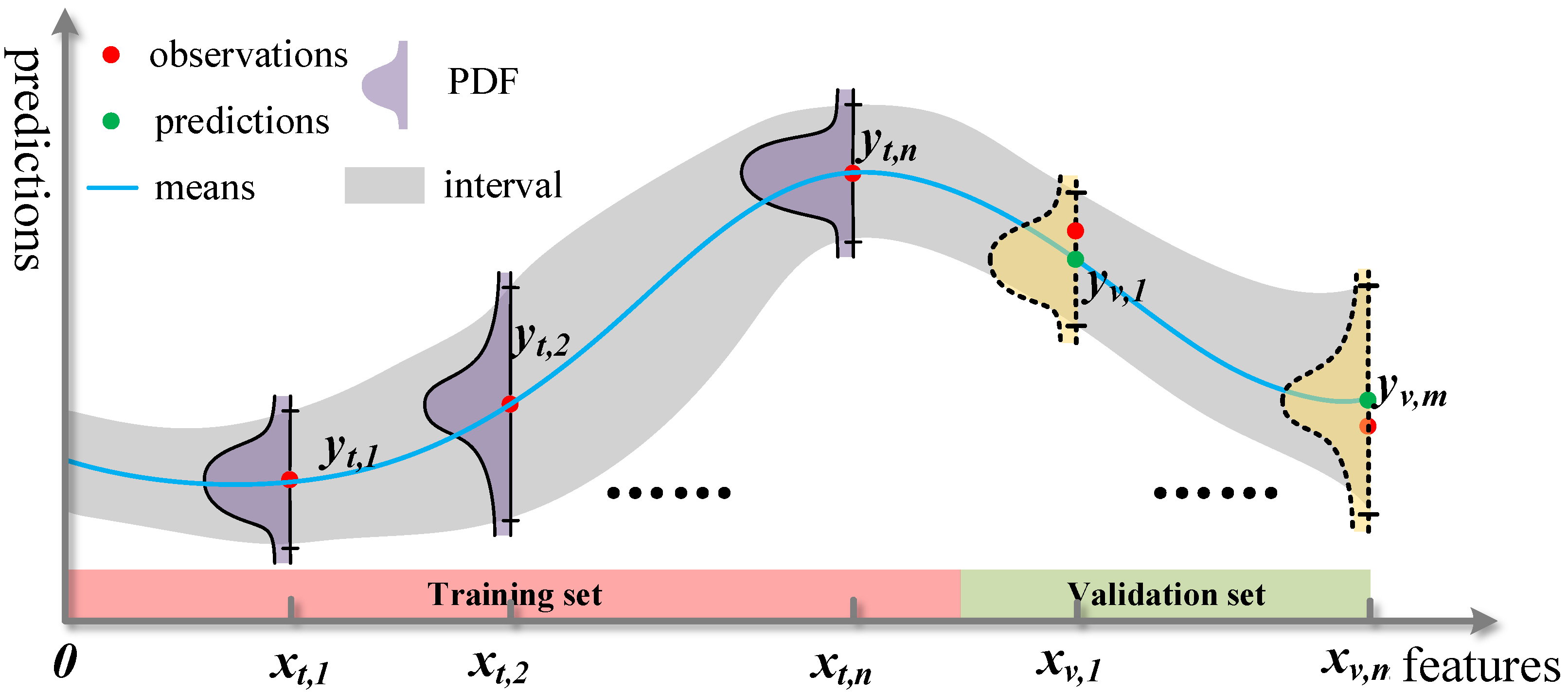
2.2. Gaussian Process Regression

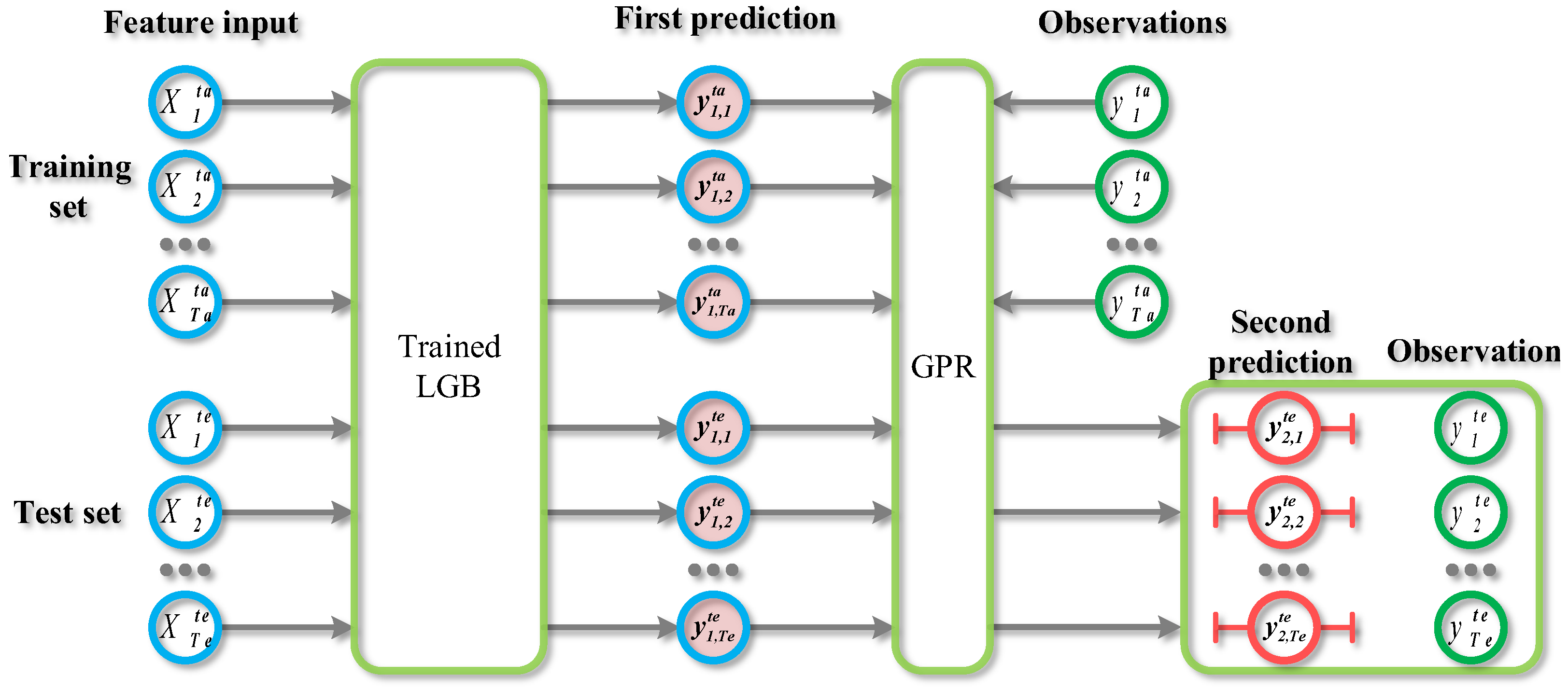
The Gaussian process regression is a nonparametric model that uses a Gaussian process prior to performing regression analysis on data. The basic principles are: assuming that the learning sample obeys the Gaussian distribution, according to the prior probability of the random variable assumed by the Gaussian distribution, estimate the posterior distribution of the random variable based on the Bayesian principle, and use the maximum likelihood method or Monte Carlo sampling to estimate the model parameters. Then, a Gaussian process regression model is constructed to obtain a probability prediction value that obeys a Gaussian distribution. The schematic diagram is shown in Figure 2.

In the figure, X = [x₁, x₂, $\dots$, x_n] represents the n-dimensional input feature vector, and Y = [y₁, y₂, $\dots$, y_n] represents the predictor variable. Suppose x and y form the following regression model:

$$y=f(X)+\epsilon ,\epsilon ~N(0,{\sigma }_n^2)$$

(8)

where $\epsilon$ is the noise and obeys the normal distribution with a mean of 0 and a variance of $\sigma$; n is the input feature dimension. The prior distribution of y^train is:

$$y^{train}~N(0,\sum (X^{train},X^{train})+{\sigma }_n^2{I}_n)$$

(9)

where $\sum$(X^train, X^train) is an n × n symmetric positive definite covariance matrix, I_n is an n-dimensional identity matrix. The detailed expression of $\sum$(X^train, X^train) is as follows:

$$\sum (X^{train},X^{train})=\left(\begin{array}{cccc}{\mathrm{cov}}_{1,1}& {\mathrm{cov}}_{1,2}& \dots & {\mathrm{cov}}_{1,n}\\ {\mathrm{cov}}_{2,1}& {\mathrm{cov}}_{2,2}& \dots & {\mathrm{cov}}_{2,n}\\ ⋮& ⋮& ⋮& ⋮\\ {\mathrm{cov}}_{n,1}& {\mathrm{cov}}_{n,2}& \dots & {\mathrm{cov}}_{n,n}\end{array}\right)$$

(10)

where cov_i,j represents the covariance between feature i and feature j. Gaussian process kernel function $\kappa$ is introduced to simulate the covariance between each feature dimension, $\sum$(X^train, X^train) = ($\kappa$_ij). In the paper, the radial basis kernel function is used, and the formula is as follows:

$${\kappa }_{RBF}(i,j)={\sigma }_f^2\exp \left[-\frac{1}{2}{(X_i-X_j)}^{T}M(X_i-X_j)\right]$$

(11)

where σ is the hyperparameter of the radial basis kernel, and M is the matrix function that characterizes the anisotropy. The joint Gaussian distribution of y^train and y^test is as follows:

$$\left[\begin{array}{l}{Y}^{train}\\ Y^{test}\end{array}\right]~N\left(0,\left[\begin{array}{l}\sum (X^{train},X^{train})+{\sigma }_n^2{I}_n\sum (X^{test},X^{train})\\ \sum (X^{train},X^{test})\sum (X^{test},X^{test})\end{array}\right]\right)$$

(12)

where $\sum (X^{train},X^{test})=\sum {(X^{test},X^{train})}^T$ is the covariance matrix between the training set feature input X^train and the test set feature input X^test, $\sum (X^{test},X^{test})$ is the internal covariance matrix of the test set feature input.

The posterior condition of the predicted value Y^test of the test set can be obtained by Bayesian inference.

$$y^{test}|y^{train}\sim N({\overline{y}}^{test},{\sigma }_{y^{test}}^2)$$

(13)

$${\overline{y}}^{test}=K_{*}{K}^{-1}{y}^{train}$$

(14)

$${\sigma }_{y^{test}}^2=K_{**}-K_{*}{K}^{-1}{K}_{*}^T$$

(15)

where $\overline{y}$^test is the predicted mean of the test set; ${\sigma }_{y^{test}}^2$ is the variance of the Gaussian distribution.

2.3. LGB-GPR

On the basis of the deterministic forecast results obtained by the LGB model, combined with the GPR method, the LGB-GPR model, which can obtain both the interval forecast results and the probabilistic forecast results, is obtained. GPR is implemented using the ‘GPy 1.9.9′ framework in python. LGB is implemented using the ‘lightgbm 3.3.1′ framework in python. All the above models were performed using ‘Intel(R) Core (TM) i7-10750H CPU @ 2.60GHz’. The flowchart of the LGB-GPR prediction is presented in Figure 3.

In Figure 3, $\left[X_1^{ta},X_2^{ta},\dots ,X_{Ta}^{ta}\right]$ represents the original training set feature input, $\left[X_1^{te},X_2^{te},\dots ,X_{Te}^{te}\right]$ represents the original test set feature input, $\left[y_{1,1}^{ta},y_{1,2}^{ta},\dots ,y_{1,Ta}^{ta}\right]$ and $\left[y_{1,1}^{te},y_{1,2}^{te},\dots ,y_{1,Te}^{te}\right]$ represents the training set results and the test set results predicted by the trained LGB model, respectively. $\left[y_1^{ta},y_2^{ta},\dots ,y_{Ta}^{ta}\right]$ represents the training set observations, $\left[y_1^{te},y_2^{te},\dots ,y_{Te}^{te}\right]$ represents the test set observations, $\left[y_{2,1}^{te},y_{2,2}^{te},\dots ,y_{2,Te}^{te}\right]$ represents the test set results predicted by the GPR model.

The prediction steps based on the LGB-GPR model are as follows:

Step1: Train LGB model with $\left[X_1^{ta},X_2^{ta},\dots ,X_{Ta}^{ta}\right]$ and $\left[y_1^{ta},y_2^{ta},\dots ,y_{Ta}^{ta}\right]$ as features and labels, respectively.

Step2: Taking $\left[X_1^{ta},X_2^{ta},\dots ,X_{Ta}^{ta}\right]$ and $\left[X_1^{te},X_2^{te},\dots ,X_{Te}^{te}\right]$ as input, respectively, use the trained LGB model to obtain $\left[y_{1,1}^{ta},y_{1,2}^{ta},\dots ,y_{1,Ta}^{ta}\right]$ and $\left[y_{1,1}^{te},y_{1,2}^{te},\dots ,y_{1,Te}^{te}\right]$.

Step3: Train the GPR model with $\left[y_{1,1}^{ta},y_{1,2}^{ta},\dots ,y_{1,Ta}^{ta}\right]$ and $\left[y_1^{ta},y_2^{ta},\dots ,y_{Ta}^{ta}\right]$.

Step4: Using the trained GPR model to get $\left[y_{2,1}^{te},y_{2,2}^{te},\dots ,y_{2,Te}^{te}\right]$, evaluate model prediction accuracy based on $\left[y_1^{te},y_2^{te},\dots ,y_{Te}^{te}\right]$ and $\left[y_{2,1}^{te},y_{2,2}^{te},\dots ,y_{2,Te}^{te}\right]$.

3. Scoring Metrics

3.1. Deterministic Forecasting Evaluation Metrics

Coefficient of certainty (R²), root mean square error (RMSE), and mean absolute percent error (MAPE) are employed to evaluate the deterministic forecasting results:

$$R^2=1-\frac{{\displaystyle \sum _{i=1}^m{\left(y_i-Y_i\right)}^2}}{{\displaystyle \sum _{i=1}^m{\left(Y_i-{\overline{Y}}_i\right)}^2}}$$

(16)

$$RMSE=\sqrt{\frac{1}{m}{\displaystyle \sum _{i=1}^m{(y_i-Y_i)}^2}}$$

(17)

$$MAPE=\frac{100\%}{m}{\displaystyle \sum _{i=1}^m\frac{\left|Y_i-y_i\right|}{Y_i}}$$

(18)

where $y_i$ and $Y_i$ are the i-th prediction and observation, respectively. $m$ is the number of validations set. The smaller the MAPE or the RMSE, the better the prediction results. The closer R² is to 1, the better the prediction results.

3.2. Probabilistic Forecasting Evaluation Metric

Interval coverage probability coefficient (ICPC) and continuous ranked probability score (CRPS) are employed to evaluate the probabilistic forecasting results:

$$ICPC=1-\frac{{\displaystyle \sum _{\alpha \in [10\%,90\%]}{\left({\displaystyle \sum _{t=1}^{T}I\left(L_t^{\alpha }\le Y_t^o\le U_t^{\alpha }\right)}/T-\alpha \right)}^2}}{{\displaystyle \sum _{\alpha \in [10\%,90\%]}{\left(\alpha -\overline{\alpha }\right)}^2}}$$

(19)

$$CRPS=\frac{1}{T}{\displaystyle \sum _{t=1}^T{\displaystyle {\int }_{-\infty }^{+\infty }{\left[F\left(y_t\right)dx-H\left(y_t-Y_t\right)\right]}^2}}d{y}_t$$

(20)

where $I\left(·\right)$ indicates the 0–1 function, which outputs 1 when the condition is met, and 0 otherwise; $L_t^{\alpha },U_t^{\alpha }$ indicate the lower and upper boundaries of the prediction interval at t period under confidence degree α, respectively; $\overline{\alpha }$ indicates the mean of the confidence degree; $F\left(·\right)$ indicates the cumulative distribution function; $H\left(·\right)$ indicates the Heaviside function. The closer the ICPC is to 1, the better the prediction interval. The smaller the CRPS, the better the uncertainty quantification results.

4. Case Study

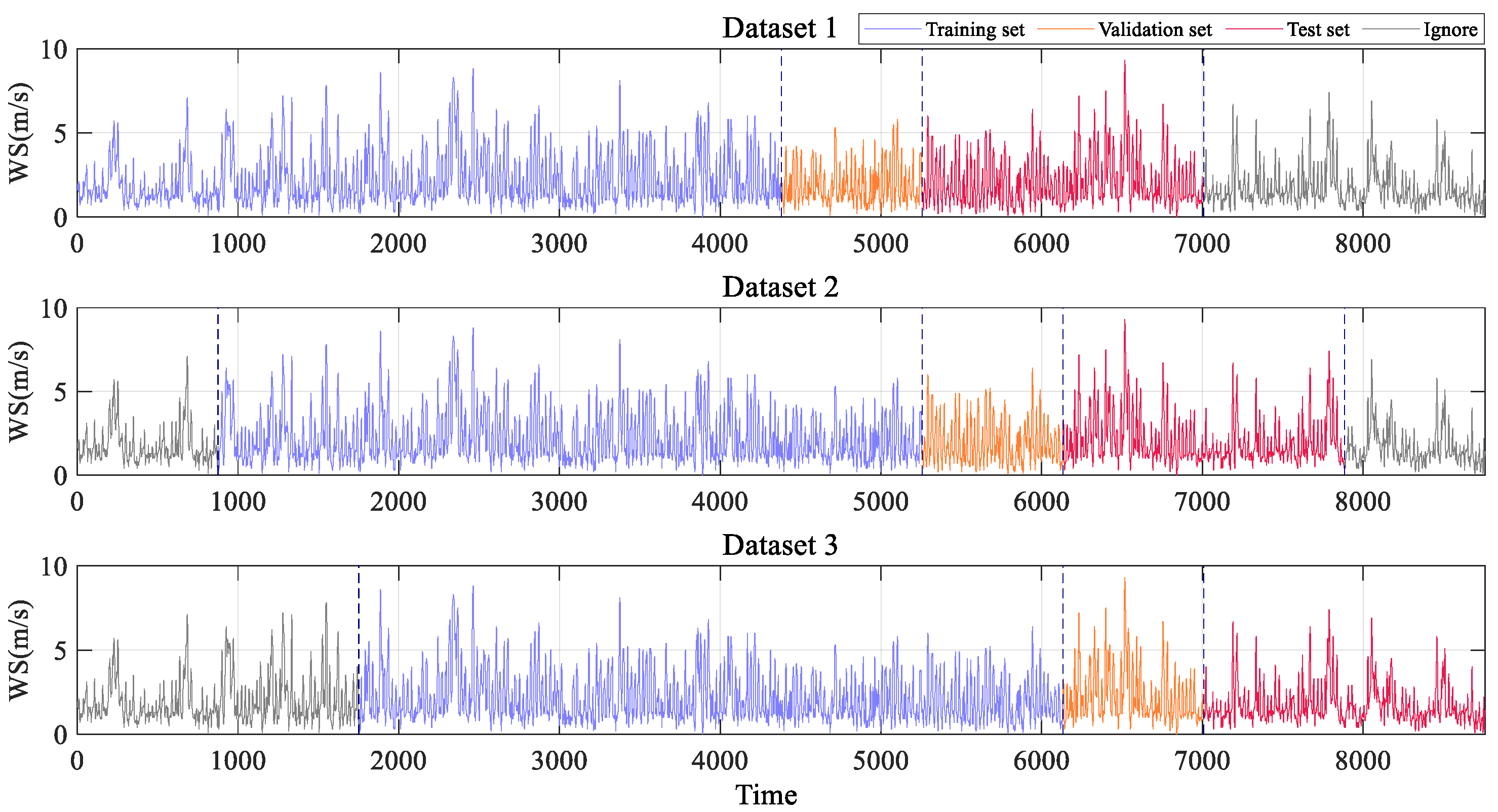
4.1. Case Introduction

To test the proposed model, a real US wind farm located at longitude W103° and latitude N38° was used for the case study. A total of 1 January 2013 to 1 January 2014 meteorological data in hourly steps, including wind speed, wind direction, temperature, dew point, relative humidity, and precipitable amount, were collected as research datasets. In this study, the historical meteorological variables of the previous 3 h were used to predict the wind-speed sequence of the next 1 h. Furthermore, to prevent overfitting, a time series sliding window method was used to partition the dataset. The sliding window size used in this study accounts for 80% of the original data, and the window slides backwards by 10% each time. In a sliding window, the data is split into training and test sets with a ratio of 6:2. A schematic diagram of the partition of the dataset is shown in Figure 4.

4.2. Data Processing

4.2.1. Data Normalized

To eliminate the influence of unit and scale differences between different meteorological datasets, the normalized data was used for calculation in the study. The normalization formula is as follows:

$$x_{norm}=\frac{x_i-x_{\min }}{x_{\max }-x_{\min }}$$

(21)

where $x_{\max }$ and $x_{\min }$ are maximum and minimum feature data, $x_{norm}$ is the normalized dataset, $x_i$ is the i-th observed data. The normalized values are in the range [0, 1].

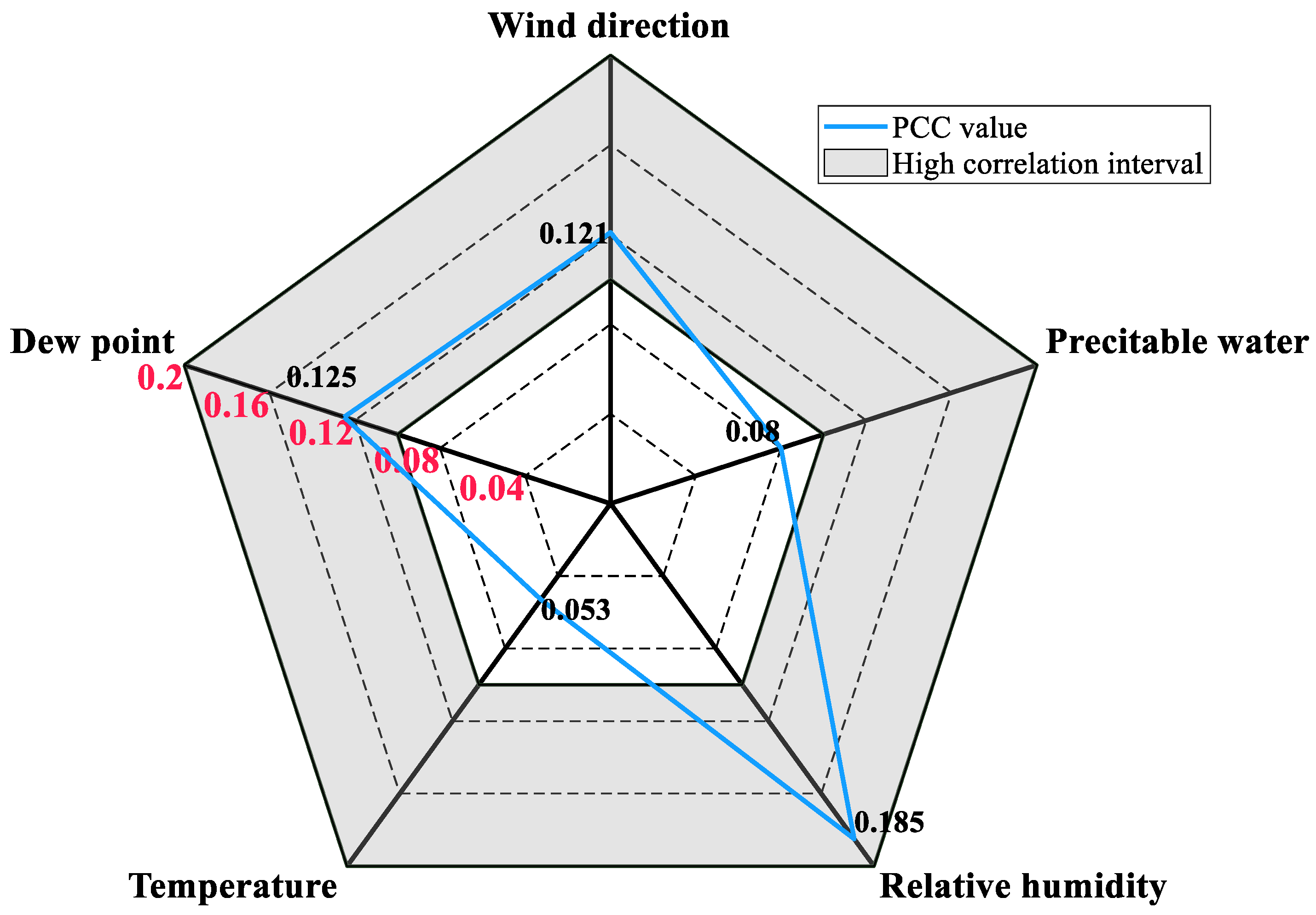
4.2.2. Feature Selection

This study involves a large amount of meteorological feature data. To reduce the computational complexity of the model and the influence of redundant features, this study uses the maximum information coefficient (MIC) to initially screen the feature vectors. The expression of MIC is as follows:

$$MIC(X_i,Y)=\underset{X_{i}Y<B(|D|)}{max}\frac{{\max }_{G}I(D|G)}{{\log }_2\min \{X_i,Y\}}$$

(22)

where $D$ is a set of ordinal pairs, $G$ is the divided grid, $D|G$ represents the probability distribution of data $D$ on grid $G$. $I(D|G)$ is the information coefficient. The range of MIC values is [0, 1], and the closer the value is to 1, the greater the correlation. In this paper, the correlation coefficient thresholds for meteorological features are set to 0.1 and 0.2.

Figure 5 shows a schematic diagram of the feature selection results. In the figure, the gray part in the figure is the high correlation interval, and the eigenvectors located in it are selected. After feature selection, feature sequences, such as dew point, relative humidity, wind direction, and wind speed, are used to train the model.

4.3. Model Selection and Hyperparameter Optimization

To verify the superiority of the proposed model, eight models, including linear regressor (LR), random forest (RF), SVR, GPR, ANN, LSTM, LGB, and LGB-GPR, were used for comparison. Among them, LR, RF, SVR, ANN, LSTM, and LGB were all point prediction models, and only point prediction results could be obtained. While GPR and LGB-GPR were probabilistic prediction models, probabilistic prediction results could be obtained. Furthermore, in order to improve the performance of the models, all the models in this study adopted a Bayesian optimization algorithm to optimize the hyperparameters.

Table 1. Model hyperparameter optimization range.

Model	Hyperparameter	Optimization Range
LGB-GPR	Tree Maximum depth	(3–15)
	Max number of leaves	(10–150)
	Learning rate	(0.005–0.2)
	Minimal number of data	(20–300)
	Kernel	(‘RBF’, ‘W’, ‘RQ’)
LGB	Tree Maximum depth	(3–15)
	Max number of leaves	(10–150)
	Learning rate	(0.005–0.2)
	Minimal number of data	(20–300)
RF	Tree Maximum depth	(3–15)
	Learning rate	(0.005–0.2)
LSTM	Hidden layer nodes	(8–32)
	Dropout	(0.01–0.5)
	Batch-size	(8–32)
	Epochs	100
	Optimizer	Adam
ANN	Hidden layer nodes	(8–32)
	Dropout	(0.01–0.5)
	Batch-size	(8–32)
	Epochs	100
	Optimizer	Adam
SVR	Kernel	(‘rbf’, ‘poly’, ‘sigmoid’)
GPR	Kernel	(‘C’, ‘RBF’, ‘RQ’)

shows the detailed hyperparameters of the eight models. The following will perform a statistical analysis of the performance of each model on multiple datasets.

5. Result and Discussion

5.1. Deterministic Prediction Result Evaluation

In this section, three indicators, R², RMSE, and MAPE, were used to evaluate the accuracy of the model’s deterministic forecast results. The scoring results of the three metrics for different models on different datasets are shown in

Table 2. R² score results statistics table.

Model (R2)	Dataset 1	Dataset 2	Dataset 3	Average
SVR	0.851	0.878	0.818	0.849
LR	0.947	0.956	0.949	0.951
RF	0.932	0.951	0.940	0.941
ANN	0.940	0.956	0.924	0.940
LSTM	0.946	0.960	0.953	0.953
LGB	0.950	0.961	0.952	0.954
GPR	0.917	0.936	0.949	0.934
LGB-GPR	0.954	0.963	0.956	0.958

,

Table 3. RMSE score results statistics table.

Model (RMSE)	Dataset 1	Dataset 2	Dataset 3	Average
SVR	0.539	0.521	0.569	0.543
LR	0.321	0.311	0.301	0.311
RF	0.364	0.331	0.328	0.341
ANN	0.342	0.311	0.368	0.340
LSTM	0.326	0.299	0.290	0.305
LGB	0.305	0.291	0.285	0.294
GPR	0.401	0.377	0.301	0.360
LGB-GPR	0.300	0.286	0.280	0.288

and

Table 4. MAPE score results statistics table.

Model (MAPE)	Dataset 1	Dataset 2	Dataset 3	Average
SVR	0.409	0.350	0.367	0.375
LR	0.156	0.138	0.136	0.143
RF	0.182	0.143	0.142	0.156
ANN	0.170	0.138	0.170	0.159
LSTM	0.167	0.133	0.141	0.147
LGB	0.156	0.130	0.119	0.135
GPR	0.209	0.170	0.130	0.170
LGB-GPR	0.152	0.128	0.118	0.133

. The best scores in the table are highlighted in bold.

It can be seen from Table 2 that the average R² value of LGB reaches 0.958, which is significantly higher than ANN’s 0.94, RF’s 0.941, and LSTM’s 0.953. In the second dataset, LGB achieved the highest R² value of 0.963, higher than SVR’s 0.878, LGB’s 0.961, and GPR’s 0.936. The above results show that the LGB model has higher R² values than the other models on all three datasets. As can be seen from Table 3, compared with the LGB model, LGB-GPR improves the accuracy of the three datasets by 1.6%, 1.7%, and 1.8%, respectively. Compared with the GPR model, LGB-GPR improves the accuracy by 24.9%, 24.1%, and 6.9% on the three datasets, respectively. The above results prove that, after combining the LGB and GPR models, the model prediction accuracy can be effectively improved. In Table 4, the performance of LGB is second only to LGB-GPR, achieving MAPE scores of 0.156, 0.130, and 0.119 on three datasets. This phenomenon shows that the LGB model itself has excellent wind-speed prediction performance, and the combination with the GPR further improves its prediction accuracy.

Figure 6 shows the prediction results of each comparison model in the three datasets for typical time periods. It can be seen from the figure that the LGB-GPR model can effectively fit the fluctuation trend of future wind speed in the three sets of datasets. This once again illustrates the superiority of LGB-GPR. In all models, the predicted results of the SVR model deviate significantly from the actual wind-speed values, which is consistent with the results in Table 2, Table 3 and Table 4.

In conclusion, the deterministic prediction score of the LGB-GPR model surpasses all the comparison models, which indicates that the LGB-GPR model can provide high-accuracy deterministic wind-speed prediction results.

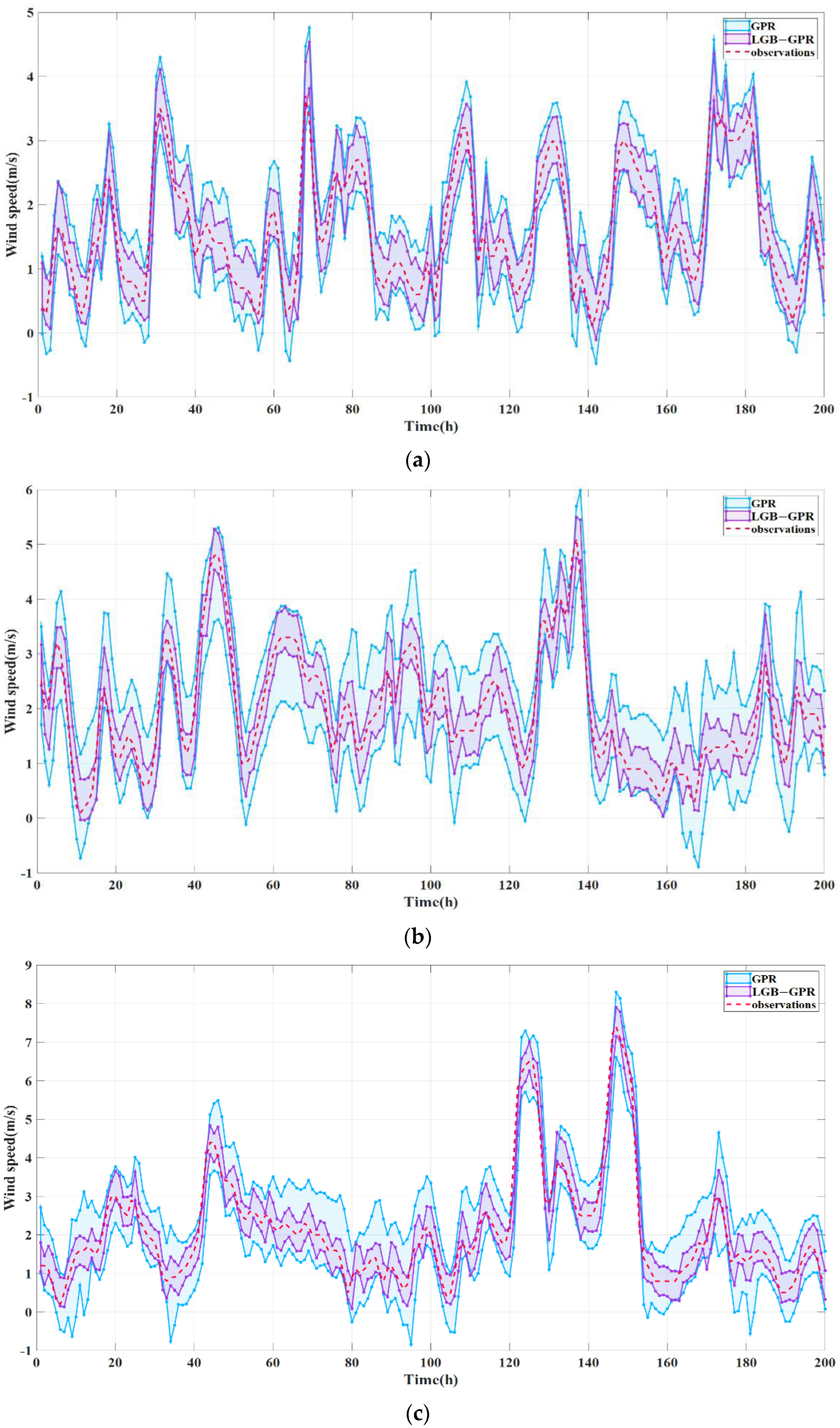
5.2. Probability Prediction Result Evaluation

In this section, two indicators, ICPC and CRPS, were used to evaluate the reliability of the model’s probability forecast results. The scoring results of two metrics for different models on different datasets are shown in

Table 5. ICPC score results statistics table.

Model (ICPC)	Dataset 1	Dataset 2	Dataset 3	Average
GPR	0.868	0.961	0.798	0.876
LGB-GPR	0.945	0.980	0.989	0.971

and

Table 6. CRPS score results statistics table.

Model (CRPS)	Dataset 1	Dataset 2	Dataset 3	Average
GPR	0.225	0.209	0.165	0.200
LGB-GPR	0.165	0.157	0.148	0.157

. The best scores in the table are highlighted in bold.

The ICPC indicator measures the appropriateness of the prediction interval of a probabilistic forecasting model. It can be seen from Table 5 that the ICPC values of the LGB-GPR model on the three datasets are 8.9%, 2.0%, and 23.9% higher than the GPR model, respectively. This shows that the probability prediction interval of the LGB-GPR model is more reasonable than that of the GPR model, and can better describe the uncertainty of the wind-speed prediction within a reasonable range. The CRPS index comprehensively measures the probability prediction and reliability of the probability prediction model. It can be seen from Table 6 that the CRPS values of the LGB-GPR model on the three datasets are lower in the GPR model, with improvements of 26%, 24.9%, and 10.3%, respectively. This result verifies the superiority of the proposed LGB-GPR model in the comprehensive performance of probabilistic forecasting.

Figure 7 shows the probabilistic prediction comparison results of the probabilistic prediction model on the three datasets. It can be seen from the figure that the probability prediction interval of the GPR model is significantly larger than that of the LGB-GPR model, which indicates that the GPR model tends to predict with greater uncertainty. However, the prediction interval of the LGB-GPR model is narrower, which indicates that the LGB-GPR model can more reliably quantify the uncertainty of wind speed.

To sum up, the probabilistic prediction results of LGB-GPR are better than the comparison model, GPR, which indicates that the LGB-GPR model can provide reliable probabilistic prediction results.

6. Conclusions

In this paper, the GPR model is introduced on the basis of the LGB model, and a wind-speed probability prediction model based on LGB-GPR is proposed. The LGB model can provide accurate deterministic wind speed prediction results, and the GPR model can provide reliable probabilistic prediction results. Combining the two can give full play to their respective advantages. This paper verifies the superiority of the LGB-GPR model from the deterministic evaluation index and the probabilistic evaluation index aspects. The results show that the LGB-GPR model outperforms all contrasting models. LGB-GPR model can not only provide high-precision deterministic forecast results, but also effectively quantify the uncertainty in wind speed forecasting, which can provide wind farm dispatchers with rich decision-making information.

References

1. Liu, G.; Qin, H.; Shen, Q.; Lyv, H.; Qu, Y.; Fu, J.; Liu, Y.; Zhou, J. Probabilistic spatiotemporal solar irradiation forecasting using deep ensembles convolutional shared weight long short-term memory network. Appl. Energy 2021, 300, 117379. [Google Scholar] [CrossRef]
2. Zhang, Z.; Ye, L.; Qin, H.; Liu, Y.; Wang, C.; Yu, X.; Yin, X.; Li, J. Wind speed prediction method using Shared Weight Long Short-Term Memory Network and Gaussian Process Regression. Appl. Energy 2019, 247, 270–284. [Google Scholar] [CrossRef]
3. Chen, J.; Zeng, G.; Zhou, W.; Du, W.; Lu, K. Wind speed forecasting using nonlinear-learning ensemble of deep learning time series prediction and extremal optimization. Energy Convers. Manag. 2018, 165, 681–695. [Google Scholar] [CrossRef]
4. Hong, Y.; Rioflorido, C.L.P.P. A hybrid deep learning-based neural network for 24-h ahead wind power forecasting. Appl. Eneryg 2019, 250, 530–539. [Google Scholar] [CrossRef]
5. Yang, Z.; Zhan, X.; Zhou, X.; Xiao, H.; Pei, Y. The Icing Distribution Characteristics Research of Tower Cross Beam of Long-Span Bridge by Numerical Simulation. Energies 2021, 14, 5584. [Google Scholar] [CrossRef]
6. Song, Y.; Zhang, M.; Øiseth, O.; Rønnquist, A. Wind deflection analysis of railway catenary under crosswind based on nonlinear finite element model and wind tunnel test. Mech. Mach. Theory 2022, 168, 104608. [Google Scholar] [CrossRef]
7. Memarzadeh, G.; Keynia, F. A new short-term wind speed forecasting method based on fine-tuned LSTM neural network and optimal input sets. Energy Convers. Manag. 2020, 213, 112824. [Google Scholar] [CrossRef]
8. Peng, Z.; Peng, S.; Fu, L.; Lu, B.; Tang, J.; Wang, K.; Li, W. A novel deep learning ensemble model with data denoising for short-term wind speed forecasting. Energy Convers. Manag. 2020, 207, 112524. [Google Scholar] [CrossRef]
9. Shahid, F.; Zameer, A.; Mehmood, A.; Raja, M.A.Z. A novel wavenets long short term memory paradigm for wind power prediction. Appl. Energy 2020, 269, 115098. [Google Scholar] [CrossRef]
10. Zhang, Z.; Qin, H.; Liu, Y.; Wang, Y.; Yao, L.; Li, Q.; Li, J.; Pei, S. Long Short-Term Memory Network based on Neighborhood Gates for processing complex causality in wind speed prediction. Energy Convers. Manag. 2019, 192, 37–51. [Google Scholar] [CrossRef]
11. Liu, G.; Tang, Z.; Qin, H.; Liu, S.; Shen, Q.; Qu, Y.; Zhou, J. Short-term runoff prediction using deep learning multi-dimensional ensemble method. J. Hydrol. 2022, 609, 127762. [Google Scholar] [CrossRef]
12. Liu, Y.; Hou, G.; Huang, F.; Qin, H.; Wang, B.; Yi, L. Directed graph deep neural network for multi-step daily streamflow forecasting. J. Hydrol. 2022, 607, 127515. [Google Scholar] [CrossRef]
13. Zhao, Y.; Ye, L.; Li, Z.; Song, X.; Lang, Y.; Su, J. A novel bidirectional mechanism based on time series model for wind power forecasting. Appl. Energy 2016, 177, 793–803. [Google Scholar] [CrossRef]
14. Wang, K.; Qi, X.; Liu, H.; Song, J. Deep belief network based k-means cluster approach for short-term wind power forecasting. Energy 2018, 165, 840–852. [Google Scholar] [CrossRef]
15. Zhang, Z.; Qin, H.; Liu, Y.; Yao, L.; Yu, X.; Lu, J.; Jiang, Z.; Feng, Z. Wind speed forecasting based on Quantile Regression Minimal Gated Memory Network and Kernel Density Estimation. Energy Convers. Manag. 2019, 196, 1395–1409. [Google Scholar] [CrossRef]
16. Liu, Y.; Qin, H.; Zhang, Z.; Pei, S.; Jiang, Z.; Feng, Z.; Zhou, J. Probabilistic spatiotemporal wind speed forecasting based on a variational Bayesian deep learning model. Appl. Energy 2020, 260, 114259. [Google Scholar] [CrossRef]
17. Optis, M.; Kumler, A.; Brodie, J.; Miles, T. Quantifying sensitivity in numerical weather prediction-modeled offshore wind speeds through an ensemble modeling approach. Wind Energy 2021, 24, 957–973. [Google Scholar] [CrossRef]
18. Yamaguchi, A.; Ishihara, T. Maximum Instantaneous Wind Speed Forecasting and Performance Evaluation by Using Numerical Weather Prediction and On-Site Measurement. Atmosphere 2021, 12, 316. [Google Scholar] [CrossRef]
19. Zhao, J.; Guo, Z.; Guo, Y.; Lin, W.; Zhu, W. A self-organizing forecast of day-ahead wind speed: Selective ensemble strategy based on numerical weather predictions. Energy 2021, 218, 119509. [Google Scholar] [CrossRef]
20. Chen, N.; Qian, Z.; Nabney, I.T.; Meng, X. Wind Power Forecasts Using Gaussian Processes and Numerical Weather Prediction. IEEE Trans. Power Syst. 2014, 29, 656–665. [Google Scholar] [CrossRef] [Green Version]
21. Niu, Z.; Yu, Z.; Tang, W.; Wu, Q.; Reformat, M. Wind power forecasting using attention-based gated recurrent unit network. Energy 2020, 196, 117081. [Google Scholar] [CrossRef]
22. Wang, J.; Wang, Y.; Li, Y. A Novel Hybrid Strategy Using Three-Phase Feature Extraction and a Weighted Regularized Extreme Learning Machine for Multi-Step Ahead Wind Speed Prediction. Energies 2018, 11, 321. [Google Scholar] [CrossRef]
23. Loukatou, A.; Howell, S.; Johnson, P.; Duck, P. Stochastic wind speed modelling for estimation of expected wind power output. Appl. Energy 2018, 228, 1328–1340. [Google Scholar] [CrossRef]
24. Jiang, W.; Yan, Z.; Feng, D.; Hu, Z. Wind speed forecasting using autoregressive moving average/generalized autoregressive conditional heteroscedasticity model: Wind speed forecasting using arma-garch model. Eur. Trans. Electr. Power 2012, 22, 662–673. [Google Scholar] [CrossRef]
25. Erdem, E.; Shi, J. ARMA based approaches for forecasting the tuple of wind speed and direction. Appl. Energy 2011, 88, 1405–1414. [Google Scholar] [CrossRef]
26. Ailliot, P.; Monbet, V. Markov-switching autoregressive models for wind time series. Environ. Model. Softw. Environ. Data News 2012, 30, 92–101. [Google Scholar] [CrossRef]
27. Arenas-López, J.P.; Badaoui, M. Stochastic modelling of wind speeds based on turbulence intensity. Renew. Energy 2020, 155, 10–22. [Google Scholar] [CrossRef]
28. Karakuş, O.; Kuruoğlu, E.E.; Altınkaya, M.A. One-day ahead wind speed/power prediction based on polynomial autoregressive model. Iet Renew. Power Gen. 2017, 11, 1430–1439. [Google Scholar] [CrossRef]
29. Tang, J.; Brouste, A.; Tsui, K.L. Some improvements of wind speed Markov chain modeling. Renew. Energy 2015, 81, 52–56. [Google Scholar] [CrossRef]
30. Azeem, A.; Fatema, N.; Malik, H.; Srivastava, S.; Malik, H.; Sharma, R. k-NN and ANN based deterministic and probabilistic wind speed forecasting intelligent approach. J. Intell. Fuzzy Syst. 2018, 35, 5021–5031. [Google Scholar] [CrossRef]
31. Vassallo, D.; Krishnamurthy, R.; Sherman, T.; Fernando, H.J.S. Analysis of Random Forest Modeling Strategies for Multi-Step Wind Speed Forecasting. Energies 2020, 13, 5488. [Google Scholar] [CrossRef]
32. Jamil, M.; Zeeshan, M. A comparative analysis of ANN and chaotic approach-based wind speed prediction in India. Neural Comput. Appl. 2018, 31, 6807–6819. [Google Scholar] [CrossRef]
33. Chen, K.; Yu, J. Short-term wind speed prediction using an unscented Kalman filter based state-space support vector regression approach. Appl. Energy 2014, 113, 690–705. [Google Scholar] [CrossRef]
34. Santamaría-Bonfil, G.; Reyes-Ballesteros, A.; Gershenson, C. Wind speed forecasting for wind farms: A method based on support vector regression. Renew. Energy 2016, 85, 790–809. [Google Scholar] [CrossRef]
35. Zhang, Y.; Pan, G.; Chen, B.; Han, J.; Zhao, Y.; Zhang, C. Short-term wind speed prediction model based on GA-ANN improved by VMD. Renew. Energy 2020, 156, 1373–1388. [Google Scholar] [CrossRef]
36. Ren, Y.; Suganthan, P.N.; Srikanth, N. A Novel Empirical Mode Decomposition With Support Vector Regression for Wind Speed Forecasting. IEEE Trans. Neural Netw. Learn. Syst. 2016, 27, 1793–1798. [Google Scholar] [CrossRef]
37. Wang, H.; Sun, J.; Sun, J.; Wang, J. Using Random Forests to Select Optimal Input Variables for Short-Term Wind Speed Forecasting Models. Energies 2017, 10, 1522. [Google Scholar] [CrossRef]
38. Shukur, O.B.; Lee, M.H. Daily wind speed forecasting through hybrid KF-ANN model based on ARIMA. Renew. Energy 2015, 76, 637–647. [Google Scholar] [CrossRef]
39. Liu, H.; Tian, H.; Li, Y. Comparison of two new ARIMA-ANN and ARIMA-Kalman hybrid methods for wind speed prediction. Appl. Energy 2012, 98, 415–424. [Google Scholar] [CrossRef]
40. Cadenas, E.; Rivera, W. Wind speed forecasting in three different regions of Mexico, using a hybrid ARIMA-ANN model. Renew. Energy 2010, 35, 2732–2738. [Google Scholar] [CrossRef]
41. Zhang, D.; Peng, X.; Pan, K.; Liu, Y. A novel wind speed forecasting based on hybrid decomposition and online sequential outlier robust extreme learning machine. Energy Convers. Manag. 2019, 180, 338–357. [Google Scholar] [CrossRef]
42. Wang, L.; Guo, Y.; Fan, M.; Li, X. Wind speed prediction using measurements from neighboring locations and combining the extreme learning machine and the AdaBoost algorithm. Energy Rep. 2022, 8, 1508–1518. [Google Scholar] [CrossRef]
Figure 1. Schematic diagram of decision tree growth strategy.
Energies 15 06942 g001
Figure 2. Schematic diagram of decision tree growth strategy.
Energies 15 06942 g002
Figure 3. LGB-GPR prediction flow chart.
Energies 15 06942 g003
Figure 4. Schematic diagram of data set division.
Energies 15 06942 g004
Figure 5. Schematic diagram of feature selection results.
Energies 15 06942 g005
Figure 6. Comparison of deterministic prediction results in typical time periods: (a) Deterministic prediction results on dataset 1; (b) deterministic prediction results on dataset 2; (c) deterministic prediction results on dataset 3.
Energies 15 06942 g006
Figure 7. Comparison of probabilistic prediction results in typical time periods: (a) Probabilistic prediction results on dataset 1; (b) probabilistic prediction results on dataset 2; (c) probabilistic prediction results on dataset 3.
Energies 15 06942 g007