

Electric Mobility Emission Reduction Policies: A Multi-Objective Optimization Assessment Approach

Abstract
:1. Introduction
- Monetary incentives for Battery electric vehicle (BEV);
- Monetary incentives for plug-in hybrid electric vehicle (PHEV);
- Governmental fleet battery electric vehicle (BEVGOV) replacement;
- Urban transit battery electric bus (BEB) replacement.
- What is the optimal allocation of different GHG reduction policies in the passenger road transportation sub-sector under varying budgets?
- What is the associated cost to achieve the 2030 GHG reduction targets?
2. Background on Optimization Approaches in GHG Reduction Policy Planning
- Firstly, a relatively straight-forward mathematical approach to transportation climate change policy decision-making. It is presented and applied to the province of Ontario, Canada but can be reformulated and applied to different jurisdictions to transparently outline the estimated costs and estimated GHG emissions reduced.
- Secondly, since a MIO approach is selected, a set of optimal solutions are generated. Hence, depending on the budget or depending on the GHG emission reduction target, the most optimal policy package can be selected with a certain range based on TCO and EV sales.
3. Methodology
3.1. Background on Canada and Ontario GHG Reduction Policies
3.2. Model Data Sources

| Parameters | Description | Justification | Value |
|---|---|---|---|
| Cost of BEV incentive ($/unit) | British Columbia EV incentive offering [47]. | $3000 | |
| Cost of PHEV incentive ($/unit) | $1500 | ||
| TCO upon replacing a provincially owned gasoline LDV to BEV ($/unit) | The difference in TCO between conventional G.LDV and BEV [48,49]. | [−$9000, −$3000] | |
| TCO upon replacing a diesel bus to BEB ($/unit) | The difference in TCO between D. Bus and BEB. Range associated with fuel price, maintenance, and market price uncertainty [50,51]. | [$50,000, $100,000] | |
| The forecasted number of LDV sales from 2020 to 2030 (#) | Forecasted value assuming historical growth in new LDV registered vehicles through years 2011–2019 [55]. The final number is reduced by 20% to account for the removal of medium-duty and heavy-light duty vehicles in the resulting value in addition to a decreasing trend in LDV sales. The ARIMA time-series method is used for forecasting [63,64]. | 7,521,535 | |
| The forecasted number of the government owned LDV in 2030 (#) | Extrapolated from the number of municipal light-duty vehicles owned in Toronto (3800) and its proportional population (20%) compared to Ontario’s population. [65] | 19,000 | |
| The forecasted number of the total LDV vehicles (including provincially owned LDV) in 2030 (#) | Forecasted value assuming historical growth in registered LDV vehicles through years 1999–2019 [56]. The final number is reduced by 10% to account for the removal of medium-duty and heavy-light duty vehicles in the resulting value. The ARIMA time-series method is used for forecasting [63,64]. | 8,902,593 | |
| The forecasted number of buses in 2030 (#) | Forecasted from Canada-wide historic urban transit bus stock growth from 2005–2019 assuming number of buses is proportion to the population in Ontario (i.e., 40% of Canada’s population) [57]. The ARIMA time-series method is used for forecasting [63,64]. | 8569 | |
| Maximum proportion of EV from the FNS of LDV (%) under a no additional provincial action scenario | The lower bound corresponds to an assumed linear growth of EV sales proportion beginning at 0.7% of the 2020 sales being EV and 40% of new vehicles being EV in 2030. For the upper bound, 2030 EV sales are assumed to be 60% of new vehicles. The upper bound represents the federal target of annual EV sales proportion [17]. It is assumed that 2 times more BEV are sold than PHEVs from 2020 to 2030. | [25%, 38%] | |
| Maximum proportion of electrified government-owned vehicle (%) | The conversion of the government LDV and bus fleets are assumed not to exceed 70%. | 70% | |
| GHG emissions in 2005 from the passenger road transportation sub-sector (g CO2 eq) | Retrieved from historic reported year 2005 GHG emissions [16,40]. Used as a baseline to compare LC GHG emission reductions in year 2020 and 2030. | 31 MT CO2 eq | |
| Maximum proportion of 2030 GHGs to 2005 GHGs (%) | A hypothetical lower bound of GHG emission reduction. Indicates a 20% reduction in 2005 levels. | 80% | |
| Minimum proportion of 2030 GHG to 2005 GHGs (%) | A hypothetical higher bound of GHG emission reduction. Indicates a 60% reduction in 2005 levels. | 40% | |
| Annual VKT by LDV (km) | Average VKT driven by average LDV and bus [54]. | 14,500 | |
| Annual VKT by bus (km) | 43,647 | ||
| Forecasted LC emission factor of LDV in 2030 per km (g CO2 eq /km) under a no additional provincial action scenario | Assumes 15.4% of fleet is EV in 2030 (i.e., 23.9% of all new LDV sales are EV in 2030). For the EV, 10.2% are BEV (39.4 g/km) and 5.2% are PHEV (78.9 g/km). The remaining proportion is assumed to be 81.5% Gasoline (176.7 g/km) and 3.1% are hybrid electric (117.8 g/km). GHG values are retrieved from GHGenius for Ontario, target year 2030, Gasoline low-sulfur LDV, Battery Electric LDV, PHEV—EV50/Gasoline50 km LDV, and HEV low-sulfur LDV [66]. | 155.83 g CO2 eq/km | |
| Forecasted LC emission factor of bus in 2030 per km (g CO2 eq /km) under a no additional provincial action scenario | Assumes 15% of bus fleet is BEB in 2030. GHG values are retrieved from GHGenius for Ontario, target year 2030, 75% Gasoline Diesel Bus (1766.3 g/km), 15% Battery Electric Bus (149.2 g/km), 7% hybrid diesel bus (1070.0 g/km), and 1% Hydrogen fuel cell (1239.1 g/km), renewable natural gas bus (546.9 g/km), and compressed natural gas bus (1474.0 g/km) [66]. | 1454.6 g CO2 eq / km | |
| Emission factor of gasoline LDV in 2030 per km (g CO2 eq /km) | GHG values are retrieved from GHGenius for Ontario, target year 2030 [66]. | 176.7 g CO2 eq/km | |
| Emission factor of EV in 2030 per km (g CO2 eq /km) | 39.4 g CO2 eq/km | ||
| Emission factor of PHEV in 2030 per km (g CO2 eq /km) | 78.9 g CO2 eq/km | ||
| Emission factor of diesel bus in 2030 per km (g CO2 eq /km) | 1766.3 g CO2 eq/km | ||
| Emission factor of BEB in 2030 per km (g CO2 eq /km) | 149.2 g CO2 eq/km |
3.3. Model Configuration
4. Results

5. Discussion on Policy Implementation
6. Conclusions
Author Contributions
Funding
Data Availability Statement
Conflicts of Interest
Abbreviations
| BEB | Battery electric bus |
| BEV | Battery electric vehicle |
| BEVGOV | Governmental fleet battery electric vehicle |
| EV | Electric vehicle (includes BEV, PHEV) |
| FNS | Forecasted number of vehicle sales |
| FNV | Forecasted number of vehicles |
| GHG | Greenhouse gases |
| LC | Life-cycle |
| LDV | Light-duty vehicles |
| MIO | Multi-objective interval optimization |
| PHEV | Plug-in hybrid electric vehicle |
| TCO | Total cost of ownership |
| VKT | Vehicle kilometers travelled |
Appendix A

References
- IPCC. Climate Change 2021: The Physical Science Basis—Summary for Policymakers; Climate Change 2021: The Physical Science Basis; Contribution of Working Group I to the Sixth Assessment Report of the Intergovernmental Panel on Climate Change; Masson-Delmotte, V., Zhai, P., Pirani, A., Connors, S.L., Péan, C., Berger, S., Caud, N., Chen, Y., Goldfarb, L., Gomis, M.I., et al., Eds.; Cambridge University Press: Cambridge, UK; New York, NY, USA, 2021; pp. 3–32. [Google Scholar] [CrossRef]
- Nasreen, S.; Mbarek, M.B.; Atiq-ur-Rehman, M. Long-Run Causal Relationship between Economic Growth, Transport Energy Consumption and Environmental Quality in Asian Countries: Evidence from Heterogeneous Panel Methods. Energy 2020, 192, 116628. [Google Scholar] [CrossRef]
- Rahman, M.M.; Vu, X.-B. The Nexus between Renewable Energy, Economic Growth, Trade, Urbanisation and Environmental Quality: A Comparative Study for Australia and Canada. Renew. Energy 2020, 155, 617–627. [Google Scholar] [CrossRef]
- Saidi, K.; Omri, A. The Impact of Renewable Energy on Carbon Emissions and Economic Growth in 15 Major Renewable Energy-Consuming Countries. Environ. Res. 2020, 186, 109567. [Google Scholar] [CrossRef]
- Rahman, M.M.; Alam, K.; Velayutham, E. Reduction of CO2 Emissions: The Role of Renewable Energy, Technological Innovation and Export Quality. Energy Rep. 2022, 8, 2793–2805. [Google Scholar] [CrossRef]
- Wang, R.; Assenova, V.A.; Hertwich, E.G. Energy System Decarbonization and Productivity Gains Reduced the Coupling of CO2 Emissions and Economic Growth in 73 Countries between 1970 and 2016. One Earth 2021, 4, 1614–1624. [Google Scholar] [CrossRef]
- Grossman, G.; Krueger, A. Environmental Impacts of a North American Free Trade Agreement; w3914; National Bureau of Economic Research: Cambridge, MA, USA, 1991. [Google Scholar] [CrossRef]
- Yang, S.; Umar, M. How Globalization Is Reshaping the Environmental Quality in G7 Economies in the Presence of Renewable Energy Initiatives? Renew. Energy 2022, 193, 128–135. [Google Scholar] [CrossRef]
- Gota, S.; Huizenga, C.; Peet, K.; Medimorec, N.; Bakker, S. Decarbonising Transport to Achieve Paris Agreement Targets. Energy Effic. 2019, 12, 363–386. [Google Scholar] [CrossRef]
- Hasan, M.A.; Frame, D.J.; Chapman, R.; Archie, K.M. Emissions from the Road Transport Sector of New Zealand: Key Drivers and Challenges. Environ. Sci. Pollut. Res. 2019, 26, 23937–23957. [Google Scholar] [CrossRef]
- IEA. Tracking Transport 2020—Analysis. IEA. Available online: https://www.iea.org/reports/tracking-transport-2020 (accessed on 27 June 2022).
- IPCC; Jaramillo, P.; Kahn Ribeiro, S.; Newman, P.; Dhar, S.; Diemuodeke, O.E.; Kajino, T.; Lee, D.S.; Nugroho, S.B.; Ou, X.; et al. Transport. In IPCC, 2022: Climate Change 2022: Mitigation of Climate Change. Contribution of Working Group III to the Sixth Assessment Report of the Intergovernmental Panel on Climate Change; Shukla, P.R., Skea, J., Slade, R., al Khourdajie, A., van Diemen, R., McCollum, D., Pathak, M., Some, S., Vyas, P., Fradera, R., et al., Eds.; Cambridge University Press: Cambridge, UK; New York, NY, USA, 2022. [Google Scholar]
- IEA. Total Final Consumption (TFC) by Sector, World (1990–2019); Data and Statistics: Explore Energy Data by Category, Indicator, Country or Region; IEA. 2020. Available online: https://www.iea.org/data-and-statistics/data-browser/?country=WORLD&fuel=Energy%20consumption&indicator=TFCShareBySector (accessed on 19 September 2022).
- Wright, D.V. Canada’s 2030 Federal Emissions Reduction Plan: A Smorgasbord of Ambition, Action, Shortcomings, and Plans to Plan. Energy Regul. Q. 2022, 10, 1–13. [Google Scholar] [CrossRef]
- Sokołowski, J.; Bouzarovski, S. Decarbonisation of the Polish Residential Sector between the 1990s and 2021: A Case Study of Policy Failures. Energy Policy 2022, 163, 112848. [Google Scholar] [CrossRef]
- Ontario. Preserving and Protecting Our Environment for Future Generations: A Made-in-Ontario Environment Plan; Ministry of the Environment, Conservation and Parks: Toronto, ON, Canada, 2018; p. 54.
- ECCC. 2030 Emissions Reduction Plan: Canada’s Next Steps to Clean Air and a Strong Economy; Environment and Climate Change Canada: Gatineau, QC, Canada, 2022; ISBN 978-0-660-42686-0.
- Crawley, M. Ford Government Quietly Releases New Plan for Hitting Climate Change Targets in Ontario|CBC News; CBC: Toronto, ON, Canada. Available online: https://www.cbc.ca/news/canada/toronto/ontario-climate-change-carbon-emissions-2030-targets-1.6419671 (accessed on 29 June 2022).
- Ontario. Ontario Emissions Scenario as of March 25, 2022; Government of Ontario: Toronto, ON, Canada, 2022; p. 3. Available online: https://prod-environmental-registry.s3.amazonaws.com/2022-04/Ontario%20Emissions%20Scenario%20as%20of%20March%2025_1.pdf (accessed on 19 September 2022).
- Plazas-Niño, F.A.; Ortiz-Pimiento, N.R.; Montes-Páez, E.G. National Energy System Optimization Modelling for Decarbonization Pathways Analysis: A Systematic Literature Review. Renew. Sustain. Energy Rev. 2022, 162, 112406. [Google Scholar] [CrossRef]
- Kang, J.; Ng, T.S.; Su, B.; Milovanoff, A. Electrifying Light-Duty Passenger Transport for CO2 Emissions Reduction: A Stochastic-Robust Input–Output Linear Programming Model. Energy Econ. 2021, 104, 105623. [Google Scholar] [CrossRef]
- Shafique, M.; Azam, A.; Rafiq, M.; Luo, X. Life Cycle Assessment of Electric Vehicles and Internal Combustion Engine Vehicles: A Case Study of Hong Kong. Res. Transp. Econ. 2022, 91, 101112. [Google Scholar] [CrossRef]
- Milovanoff, A.; Posen, I.D.; MacLean, H.L. Electrification of Light-Duty Vehicle Fleet Alone Will Not Meet Mitigation Targets. Nat. Clim. Chang. 2020, 10, 1102–1107. [Google Scholar] [CrossRef]
- Soukhov, A.; Mohamed, M. Occupancy and GHG Emissions: Thresholds for Disruptive Transportation Modes and Emerging Technologies. Transp. Res. Part Transp. Environ. 2022, 102, 103127. [Google Scholar] [CrossRef]
- Mustapa, S.I.; Bekhet, H.A. Analysis of CO2 Emissions Reduction in the Malaysian Transportation Sector: An Optimisation Approach. Energy Policy 2016, 89, 171–183. [Google Scholar] [CrossRef]
- Sen, B.; Ercan, T.; Tatari, O.; Zheng, Q.P. Robust Pareto Optimal Approach to Sustainable Heavy-Duty Truck Fleet Composition. Resour. Conserv. Recycl. 2019, 146, 502–513. [Google Scholar] [CrossRef]
- Karan, E.; Asadi, S.; Ntaimo, L. A Stochastic Optimization Approach to Reduce Greenhouse Gas Emissions from Buildings and Transportation. Energy 2016, 106, 367–377. [Google Scholar] [CrossRef]
- Cristóbal, J.; Guillén-Gosálbez, G.; Kraslawski, A.; Irabien, A. Stochastic MILP Model for Optimal Timing of Investments in CO2 Capture Technologies under Uncertainty in Prices. Energy 2013, 54, 343–351. [Google Scholar] [CrossRef]
- Zeng, Y.; Cai, Y.; Huang, G.; Dai, J. A Review on Optimization Modeling of Energy Systems Planning and GHG Emission Mitigation under Uncertainty. Energies 2011, 4, 1624–1656. [Google Scholar] [CrossRef]
- Chen, J.P.; Huang, G.; Baetz, B.W.; Lin, Q.G.; Dong, C.; Cai, Y.P. Integrated Inexact Energy Systems Planning under Climate Change: A Case Study of Yukon Territory, Canada. Appl. Energy 2018, 229, 493–504. [Google Scholar] [CrossRef]
- Li, Y.P.; Huang, G.H.; Chen, X. An Interval-Valued Minimax-Regret Analysis Approach for the Identification of Optimal Greenhouse-Gas Abatement Strategies under Uncertainty. Energy Policy 2011, 39, 4313–4324. [Google Scholar] [CrossRef]
- Rommelfanger, H. Fuzzy Linear Programming and Applications. Eur. J. Oper. Res. 1996, 92, 512–527. [Google Scholar] [CrossRef]
- Tan, R.R.; Culaba, A.B.; Aviso, K.B. A Fuzzy Linear Programming Extension of the General Matrix-Based Life Cycle Model. J. Clean. Prod. 2008, 16, 1358–1367. [Google Scholar] [CrossRef]
- Tan, R.R.; Ballacillo, J.A.B.; Aviso, K.B.; Culaba, A.B. A Fuzzy Multiple-Objective Approach to the Optimization of Bioenergy System Footprints. Chem. Eng. Res. Des. 2009, 87, 1162–1170. [Google Scholar] [CrossRef]
- Martinsen, D.; Krey, V. Compromises in Energy Policy-Using Fuzzy Optimization in an Energy Systems Model. Energy Policy 2008, 36, 2983–2994. [Google Scholar] [CrossRef]
- Davis, M.; Ahiduzzaman, M.; Kumar, A. How to Model a Complex National Energy System? Developing an Integrated Energy Systems Framework for Long-Term Energy and Emissions Analysis. Int. J. Glob. Warm. 2019, 17, 23. [Google Scholar] [CrossRef]
- Vaillancourt, K.; Alcocer, Y.; Bahn, O.; Fertel, C.; Frenette, E.; Garbouj, H.; Kanudia, A.; Labriet, M.; Loulou, R.; Marcy, M.; et al. A Canadian 2050 Energy Outlook: Analysis with the Multi-Regional Model TIMES-Canada. Appl. Energy 2014, 132, 56–65. [Google Scholar] [CrossRef]
- Jaccard, M.; Loulou, R.; Kanudia, A.; Nyboer, J.; Bailie, A.; Labriet, M. Methodological Contrasts in Costing Greenhouse Gas Abatement Policies: Optimization and Simulation Modeling of Micro-Economic Effects in Canada. Eur. J. Oper. Res. 2003, 145, 148–164. [Google Scholar] [CrossRef]
- ECCC. Canada’s Fourth Biennial Report to the United Nations Framework Convention on Climate Change (UNFCCC); Environment and Climate Change Canada: Gatineau, QC, Canada, 2019. Available online: https://unfccc.int/sites/default/files/resource/br4_final_en.pdf (accessed on 19 September 2022).
- ECCC. National Inventory Report 1990–2019: Greenhouse Gas Sources and Sinks in Canada; Environment and Climate Change Canada: Gatineau, QC, Canada, 2021.
- Ontario. Ontario Paves the Way for Electric Vehicles. Newsroom. 2020. Available online: https://news.ontario.ca/en/release/12732/ontario-paves-the-way-for-electric-vehicles (accessed on 19 December 2020).
- Ontario. Eligible Electric Vehicle Charging Stations. 2020. Available online: http://www.mto.gov.on.ca/english/vehicles/electric/electric-vehicle-charging-stations.shtml (accessed on 20 December 2020).
- City of Toronto. City of Toronto Electric Vehicle Strategy: Supporting the City in Achieving Its TransformTO Transportation Goals; City of Toronto, Canada. 2019. Available online: https://www.toronto.ca/wp-content/uploads/2020/02/8c46-City-of-Toronto-Electric-Vehicle-Strategy.pdf (accessed on 19 September 2022).
- City of Ottawa. Climate Change Master Plan; City of Ottawa, Canada. 2020. Available online: https://documents.ottawa.ca/sites/documents/files/climate_change_mplan_en.pdf (accessed on 19 September 2022).
- City of Kingston. Electrify City’s Fleet; City of Kingston, Canada. 2020. Available online: https://www.cityofkingston.ca/apps/councilpriorities/climate_electrifyfleet.html (accessed on 20 December 2020).
- Greater Sudbury. Greater Sudbury Community Energy and Emissions Plan; Greater Sudbury, Canada. 2019; Available online: https://www.greatersudbury.ca/sites/sudburyen/assets/File/Comms/FINAL%20Greater%20Sudbury%20CEEP.pdf (accessed on 19 September 2022).
- British Columbia. Go Electric Program. Available online: https://www2.gov.bc.ca/gov/content/industry/electricity-alternative-energy/transportation-energies/clean-transportation-policies-programs/clean-energy-vehicle-program (accessed on 20 December 2020).
- Plug’n Drive. Electric Vehicle FAQ—Plug’n Drive. Plug ‘n Drive, Canada. Available online: https://www.plugndrive.ca/electric-vehicle-faq/ (accessed on 20 December 2020).
- Lutsey, N.; Nicholas, M. Update on Electric Vehicle Costs in the United States through 2030; ICCT: Binangonan, Philippines, 2019; Available online: https://theicct.org/wp-content/uploads/2021/06/EV_cost_2020_2030_20190401.pdf (accessed on 19 September 2022).
- Mohamed, M.; Ferguson, M.; Kanaroglou, P. What Hinders Adoption of the Electric Bus in Canadian Transit? Perspectives of Transit Providers. Transp. Res. Part Transp. Environ. 2018, 64, 134–149. [Google Scholar] [CrossRef]
- Quarles, N.; Kockelman, K.M.; Mohamed, M. Costs and Benefits of Electrifying and Automating Bus Transit Fleets. Sustainability 2020, 12, 3977. [Google Scholar] [CrossRef]
- S&T Squared Consultants Inc. GHGenius; S&T Squared Consultants Inc.: San Jose, CA, USA, 2022. [Google Scholar]
- ECCC. Canadian Environmental Sustainability Indicators: Greenhouse Gas Emissions. Environment and Climate Change Canada. Environment and Climate Change Canada. Available online: https://www.canada.ca/en/environment-climate-change/services/environmental-indicators/greenhouse-gas-emissions.html (accessed on 1 December 2020).
- USDOE. Average Annual Vehicle Miles Traveled by Major Vehicle Category; US Department of Energy: Energy Efficiency and Renewable Energy; United States Department of Energy. 2020. Available online: https://afdc.energy.gov/data/ (accessed on 10 January 2021).
- Statistics Canada. Table 20-10-0021-01 New Motor Vehicle Registrations; Statistics Canada: Ottawa, ON, Canada, 2022. [CrossRef]
- Statistics Canada. Table 23-10-0067-01 Vehicle Registrations, by Type of Vehicle. Statistics Canada: Ottawa, ON, Canada, 2020. [Google Scholar] [CrossRef]
- Statistics Canada. Table 23-10-0086-01 Canadian Passenger Bus and Urban Transit Industries, Equipment Operated, by Industry and Type of Vehicle. Statistics Canada: Ottawa, ON, Canada, 2022. [Google Scholar] [CrossRef]
- TTC—Service Planning and Scheduling Department. TTC Service Summary—June 21, 2020 to September 5, 2020; Service Summary Report; Toronto Transit Commission, Canada: Toronto, ON, Canada, 2020. [Google Scholar]
- City of Mississauga. MiWay Furthers the City’s Commitment to Climate Change with First-Ever 60 Foot Hybrid-Electric Buses in Ontario; City of Mississauga, Canada. 2020. Available online: https://www.mississauga.ca/city-of-mississauga-news/news/miway-furthers-the-citys-commitment-to-climate-change-with-first-ever-60-foot-hybrid-electric-buses-in-ontario/ (accessed on 2 August 2022).
- Hamilton, H.; Chard, R.; Lee, B.; Silver, F.; Slosky, J. The Advanced Technology Transit Bus Index: A North American Zeb Inventory Report; Calstart: Padadena, CA, USA, 2021. [Google Scholar]
- Kouniakis, A. New Garbage-Fuelled HSR Bus Hits Hamilton’s Streets. 2020. Available online: https://www.insauga.com/new-garbage-fuelled-hsr-bus-hits-hamiltons-streets/ (accessed on 2 August 2022).
- CALSTART Inc. Canada Doubles Zero-Emission Bus Fleet, Adding 307 New Full-Size Buses Since 2020. Newswire. Available online: https://www.newswire.ca/news-releases/canada-doubles-zero-emission-bus-fleet-adding-307-new-full-size-buses-since-2020-857327438.html (accessed on 2 August 2022).
- Hyndman, R.; Athanasopoulos, G.; Bergmeir, C.; Caceres, G.; Chhay, L.; O’Hara-Wild, M.; Petropoulos, F.; Razbash, S.; Wang, E.; Yasmeen, F. Forecast: Forecasting Functions for Time Series and Linear Models; CRAN: Windhoek, Namibia, 2022. [Google Scholar]
- Hyndman, R.J.; Khandakar, Y. Automatic Time Series Forecasting: The Forecast Package for R. J. Stat. Softw. 2008, 27, 1–22. [Google Scholar] [CrossRef]
- City of Toronto. The Pathway to Sustainable City of Toronto Fleets; City of Toronto, Canada. 2020. Available online: https://www.toronto.ca/city-government/accountability-operations-customer-service/long-term-vision-plans-and-strategies/green-fleet-plan/ (accessed on 20 May 2022).
- S&T Squared Consultants Inc. GHGenius 5.0a. Available online: https://ghgenius.ca/ (accessed on 20 May 2022).
- Alves, M.J.; Clímaco, J. A Review of Interactive Methods for Multiobjective Integer and Mixed-Integer Programming. Eur. J. Oper. Res. 2007, 180, 99–115. [Google Scholar] [CrossRef]
- El-sobky, B.; Abo-elnaga, Y.; Elsaid, A.; Foda, A. Relaxed I-SHOT Trust-Region Algorithm for Solving Multi-Objective Economic Emission Load Dispatch Problem. J. Taibah Univ. Sci. 2018, 12, 573–583. [Google Scholar] [CrossRef]
- Ontario. Ontario’s Plan to Build. news.ontario.ca. Available online: https://news.ontario.ca/en/release/1002123/ontarios-plan-to-build (accessed on 4 July 2022).
- The Canadian Press. Ontario Liberals Pledge to Build, Repair Schools with $10 Billion from Scrapping Highway 413; CBC, Toronto, Canada. Available online: https://www.cbc.ca/news/canada/toronto/ontario-liberals-schools-repairs-highway-413-1.6440928 (accessed on 4 July 2022).
- Vice, M.; Mikolášik, M. Technological Advancements Within the Canadian Electric Vehicle Industry. Dev. Inf. Knowl. Manag. Bus. Appl. 2022, 377, 569–600. [Google Scholar] [CrossRef]
- Ebie, E.; Ewumi, O. Electric Vehicle Viability: Evaluated for a Canadian Subarctic Region Company. Int. J. Environ. Sci. Technol. 2022, 19, 2573–2582. [Google Scholar] [CrossRef]
- Bittencourt, T.A.; Giannotti, M. The Unequal Impacts of Time, Cost and Transfer Accessibility on Cities, Classes and Races. Cities 2021, 116, 103257. [Google Scholar] [CrossRef]
- Ashik, F.R.; Rahman, M.H.; Kamruzzaman, M. Investigating the Impacts of Transit-Oriented Development on Transport-Related CO2 Emissions. Transp. Res. Part Transp. Environ. 2022, 105, 103227. [Google Scholar] [CrossRef]
- Cheng, H.; Mao, C.; Madanat, S.; Horvath, A. Minimizing the Total Costs of Urban Transit Systems Can Reduce Greenhouse Gas Emissions: The Case of San Francisco. Transp. Policy 2018, 66, 40–48. [Google Scholar] [CrossRef]
- Dulal, H.B.; Brodnig, G.; Onoriose, C.G. Climate Change Mitigation in the Transport Sector through Urban Planning: A Review. Habitat Int. 2011, 35, 494–500. [Google Scholar] [CrossRef]
- Pan, H.; Page, J.; Zhang, L.; Cong, C.; Ferreira, C.; Jonsson, E.; Näsström, H.; Destouni, G.; Deal, B.; Kalantari, Z. Understanding Interactions between Urban Development Policies and GHG Emissions: A Case Study in Stockholm Region. Ambio 2020, 49, 1313–1327. [Google Scholar] [CrossRef]
- Turoń, K.; Czech, P. The Concept of Rules and Recommendations for Riding Shared and Private E-Scooters in the Road Network in the Light of Global Problems. In Modern Traffic Engineering in the System Approach to the Development of Traffic Networks; Advances in Intelligent Systems and Computing; Macioszek, E., Sierpiński, G., Eds.; Springer International Publishing: Cham, Germany, 2020; Volume 1083, pp. 275–284. [Google Scholar] [CrossRef]
- Faherty, T.; Morrissey, J. Challenges to Active Transport in a Car-Dependent Urban Environment: A Case Study of Auckland, New Zealand. Int. J. Environ. Sci. Technol. 2014, 11, 2369–2386. [Google Scholar] [CrossRef]
- Turoń, K. Social Barriers and Transportation Social Exclusion Issues in Creating Sustainable Car-Sharing Systems. Entrep. Sustain. Issues 2021, 9, 10–22. [Google Scholar] [CrossRef]
- Liu, X.; Xu, W. Adoption of Ride-Sharing Apps by Chinese Taxi Drivers and Its Implication for the Equality and Wellbeing in the Sharing Economy. Chin. J. Commun. 2019, 12, 7–24. [Google Scholar] [CrossRef]
- Cole, R.; Burke, M.; Leslie, E.; Donald, M.; Owen, N. Perceptions of Representatives of Public, Private, and Community Sector Institutions of the Barriers and Enablers for Physically Active Transport. Transp. Policy 2010, 17, 496–504. [Google Scholar] [CrossRef]
- Chowdhury, S.; Zhai, K.; Khan, A. The Effects of Access and Accessibility on Public Transport Users’ Attitudes. J. Public Transp. 2016, 19, 97–113. [Google Scholar] [CrossRef]
- Zhu, Q.; Leibowicz, B.D.; Busby, J.W.; Shidore, S.; Adelman, D.E.; Olmstead, S.M. Enhancing Policy Realism in Energy System Optimization Models: Politically Feasible Decarbonization Pathways for the United States. Energy Policy 2022, 161, 112754. [Google Scholar] [CrossRef]
| Provincial Policies (Ontario) | Federal Policies (Canada) | |||||
|---|---|---|---|---|---|---|
| Policy | Cost * | Outcome | Source | Policy | Outcome | Source |
| BEV incentive | $3000 point-of-purchase incentive per BEV. | An increase in one BEV and a reduction in one conventional gasoline LDV. | [47] | Carbon price | An increase in the proportion of EV sold and reduction in conventional vehicles use due to increased fossil fuel price. | [39] |
| PHEV incentive | $1500 point-of-purchase incentive per PHEV. | An increase in one PHEV and a reduction in one conventional gasoline LDV. | [47] | iZEV Program | Additional point-of-purchase incentives will further increase the proportion of EV sold and reduction in gasoline LDV ($5000 BEV, $2500 PHEV). | [39] |
| BEVGov Replacement | Between $9000 to $3000 saved per BEV (compared to conventional gasoline LDV) depending on TCO A. | Retire conventional gasoline LDV and replace with BEV. | [48,49] | Passenger Automobile and Light Truck Greenhouse Gas Emission Regulations | Incremental reduction in operational emission intensity of gasoline LDV (Model year 2011 to 2025). | [39] |
| BEB Replacement | Between $50,000 to $100,000 per BEB (compared to conventional diesel bus) depending on TCO B. | Retire conventional bus and replace with BEB. | [50,51] | Clean Fuel Standard | Incremental reduction in emission intensity of fossil fuel combustion. | [39] |
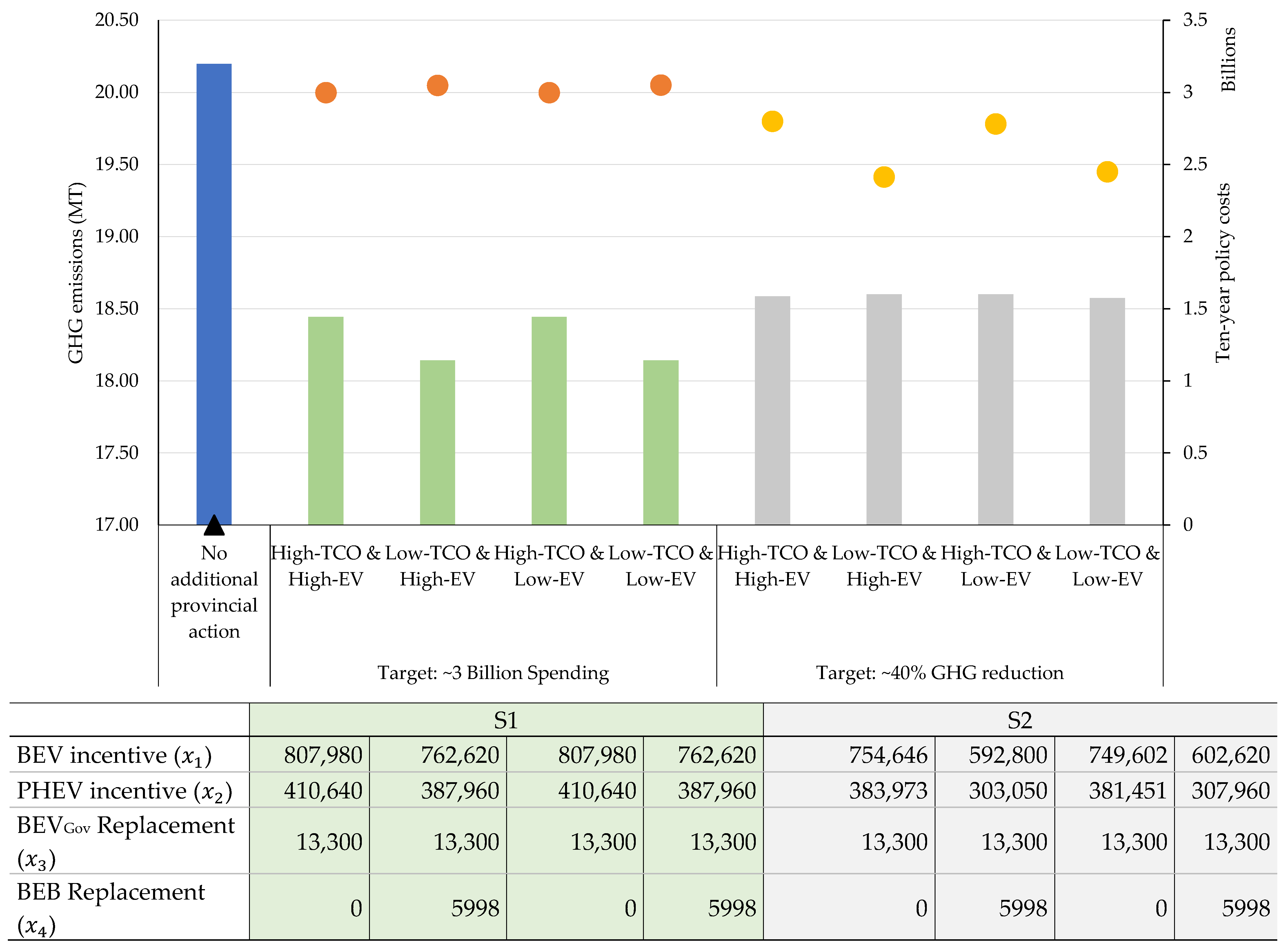
| Policy Intervention | Policy Units (Over Ten Years) | Proportion of GHG Emission Reductions (in Year 2030 Relative to Each Policy Scenario) | Proportion of Cost | GHG Reduction Efficiency ($/T CO2eq Reduced) A | |||
|---|---|---|---|---|---|---|---|
| S1 | S2 | S1 | S2 | S1 | S2 | S1 and S2 | |
| BEV incentive | 762,620 to 807,980 | 592,800 to 754,646 | 60% to 73% | 57% to 72% | 75% to 81% | 74% to 81% | 1507 |
| PHEV incentive | 387,960 to 410,640 | 303,050 to 383,973 | 22% to 26% | 21% to 26% | 19% to 21% | 19% to 21% | 1058 |
| BEVGov Replacement | 13,300 | 13,300 | 1% | 1% | −1% to −4% | −1% to −5% | −4521 to −1507 |
| BEB Replacement | 0 to 5998 | 5998 | 0% to 17% | 0% to 21% | 0% to 10% | 0% to 12% | 780 to 1417 |
Publisher’s Note: MDPI stays neutral with regard to jurisdictional claims in published maps and institutional affiliations. |
© 2022 by the authors. Licensee MDPI, Basel, Switzerland. This article is an open access article distributed under the terms and conditions of the Creative Commons Attribution (CC BY) license (https://creativecommons.org/licenses/by/4.0/).
Share and Cite
Soukhov, A.; Foda, A.; Mohamed, M. Electric Mobility Emission Reduction Policies: A Multi-Objective Optimization Assessment Approach. Energies 2022, 15, 6905. https://doi.org/10.3390/en15196905
Soukhov A, Foda A, Mohamed M. Electric Mobility Emission Reduction Policies: A Multi-Objective Optimization Assessment Approach. Energies. 2022; 15(19):6905. https://doi.org/10.3390/en15196905
Chicago/Turabian StyleSoukhov, Anastasia, Ahmed Foda, and Moataz Mohamed. 2022. "Electric Mobility Emission Reduction Policies: A Multi-Objective Optimization Assessment Approach" Energies 15, no. 19: 6905. https://doi.org/10.3390/en15196905
APA StyleSoukhov, A., Foda, A., & Mohamed, M. (2022). Electric Mobility Emission Reduction Policies: A Multi-Objective Optimization Assessment Approach. Energies, 15(19), 6905. https://doi.org/10.3390/en15196905