

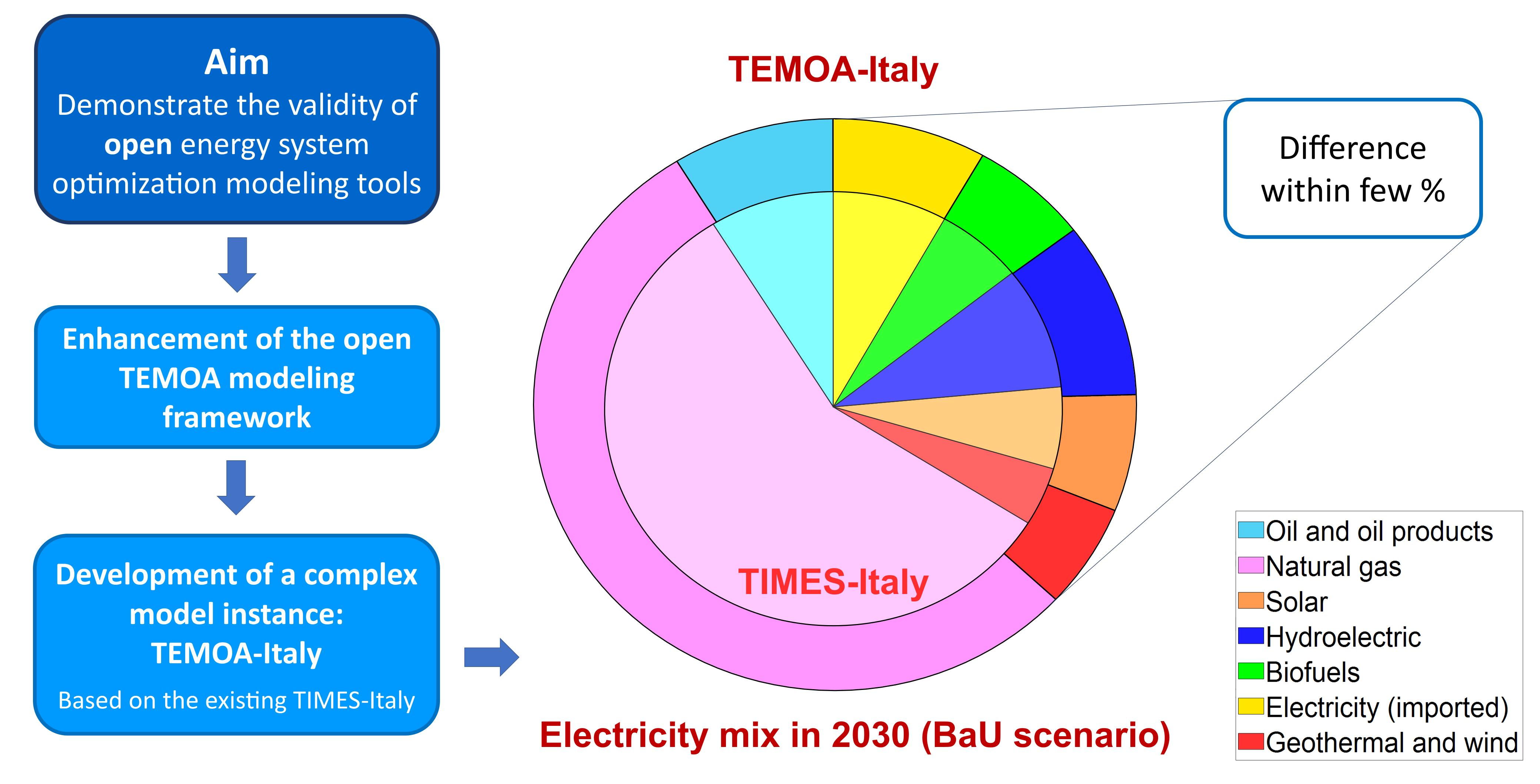
Can We Rely on Open-Source Energy System Optimization Models? The TEMOA-Italy Case Study


Abstract
:
1. Introduction
TIMES and Open-Source Energy System Optimization Modeling Frameworks
2. Methodology
2.1. Selection of the Open-Source Framework
2.2. Enhancement of the TEMOA Framework
- Labels used for internal database processing identify the different kinds of commodities (physical, demand, emissions) and technologies (“supply-side” or “demand-side” sectors), and the belonging of each time period to the set of “existing” or “future” years. More in detail, existing (historical) periods represent a base for the model where the energy system configuration at a certain point in time can be defined and has no freedom neither associated investment costs as the existing technologies are already present in the energy system when the analysis begins. Existing periods are also used to calibrate the energy-use features of the technologies included in the model, based on energy statistics. Future periods, on the other hand, represent the optimization horizon in which the total cost of the system has to be minimized.
- Sets associate definite entities to the labels mentioned above. In TEMOA there are mainly four kinds of sets: periods, sub-annual “time slices”, technologies, and energy commodities. Periods require to assign the definition of the milestone years considered as representative of each period. Then, sub-annual time slices subdivide each period into portions of the day (day, night, and peak) and seasons of the year in order to better tune the model of the supply part of the RES under exam. Indeed, production features of some technologies (e.g., renewable plants) can strongly vary according to the seasonal or daily time slices in which they operate. The technologies set contains the definition of all the possible energy technologies that the model can build, and the commodity set contains the definition of all the input and output forms of energy that the different technologies consume and produce.
- Parameters can be used to define processes or constraints, thus, to assign techno-economic features, or to assign upper or lower bounds for technologies’ evolution.
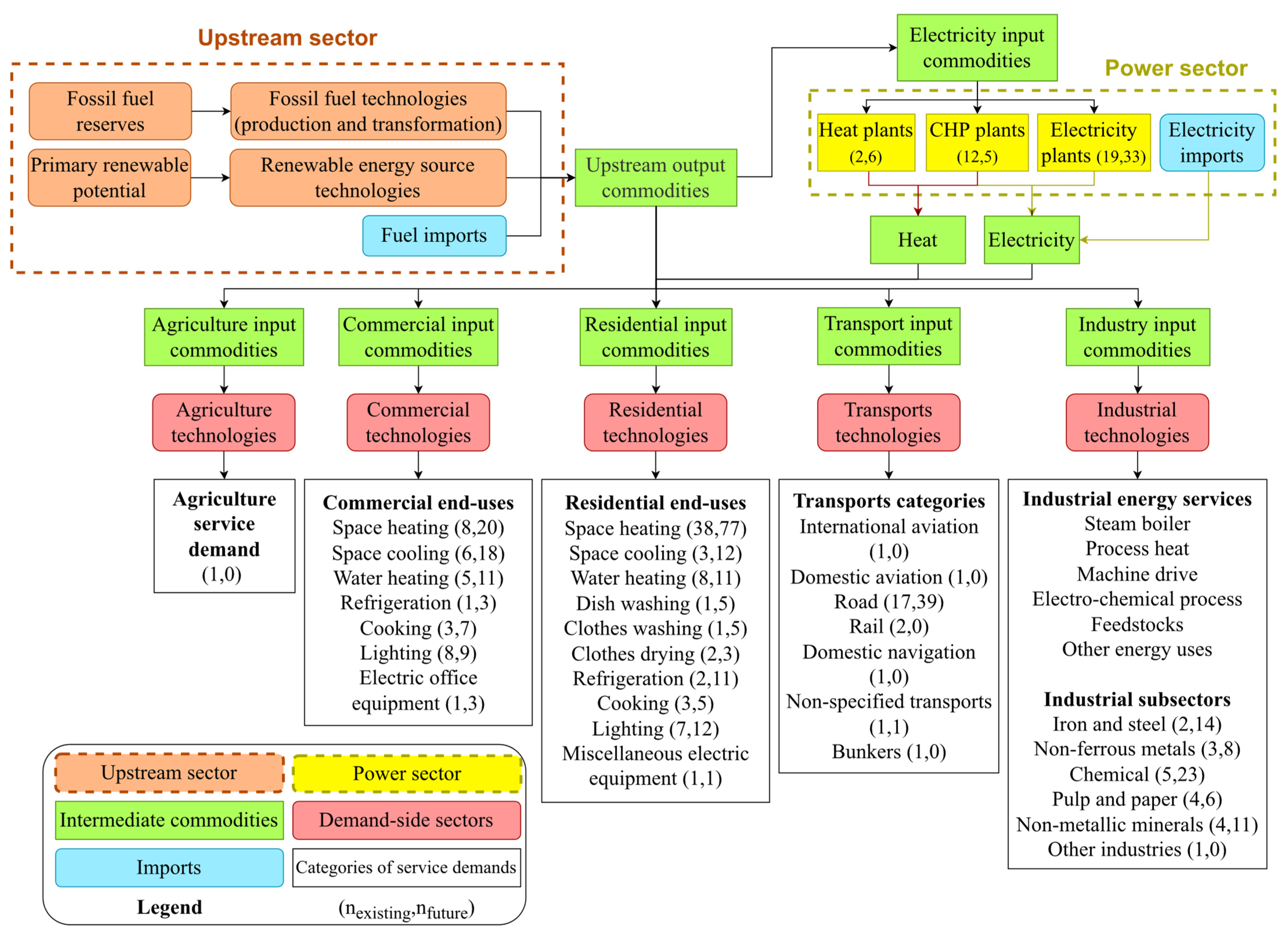
3. Case Study: The Italian Energy System
4. Comparison of Results
- Medium level-costs for import of primary sources [58].
- No subsidies to renewable electricity production.
- Neither emission limits, nor carbon tax applied.
- No carbon capture, utilization, and storage technologies.
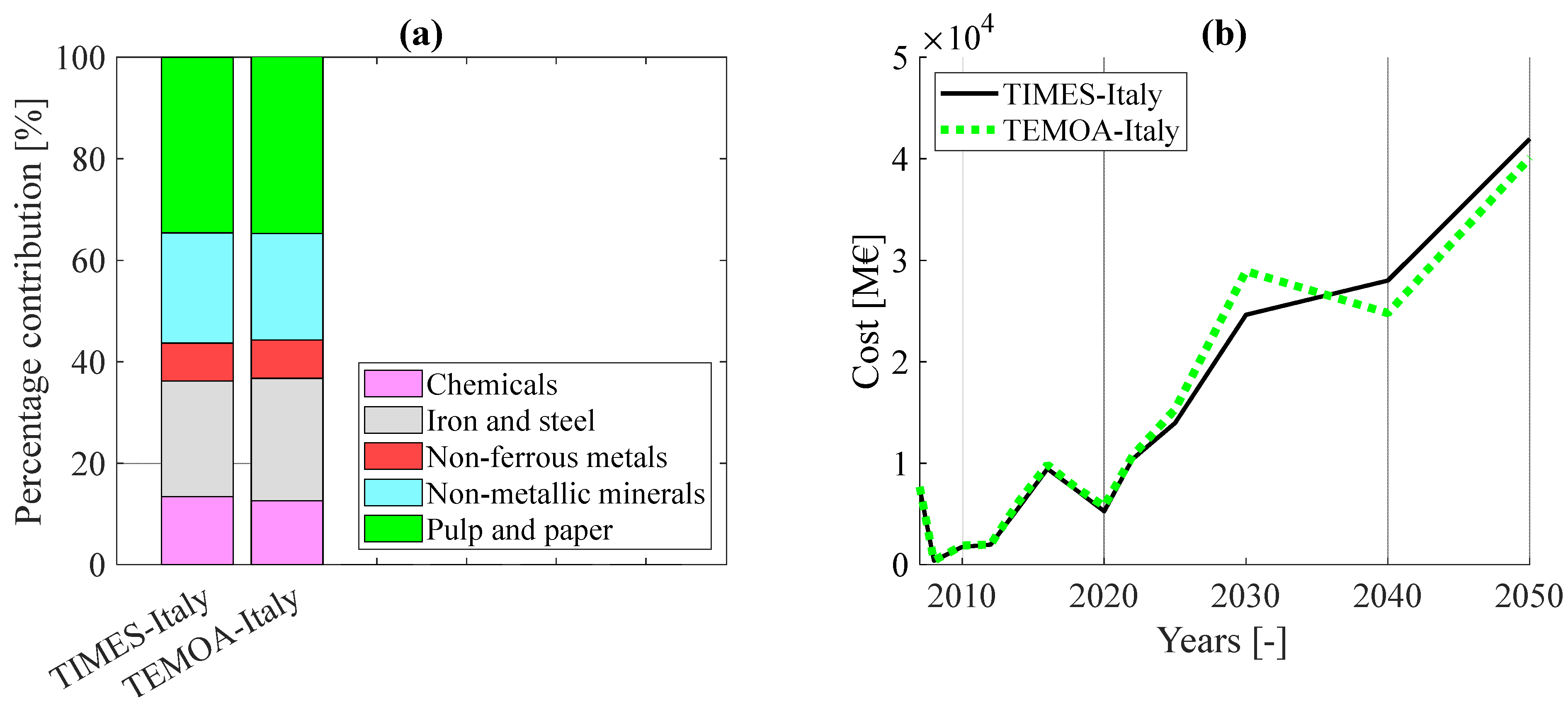
4.1. Computational Cost
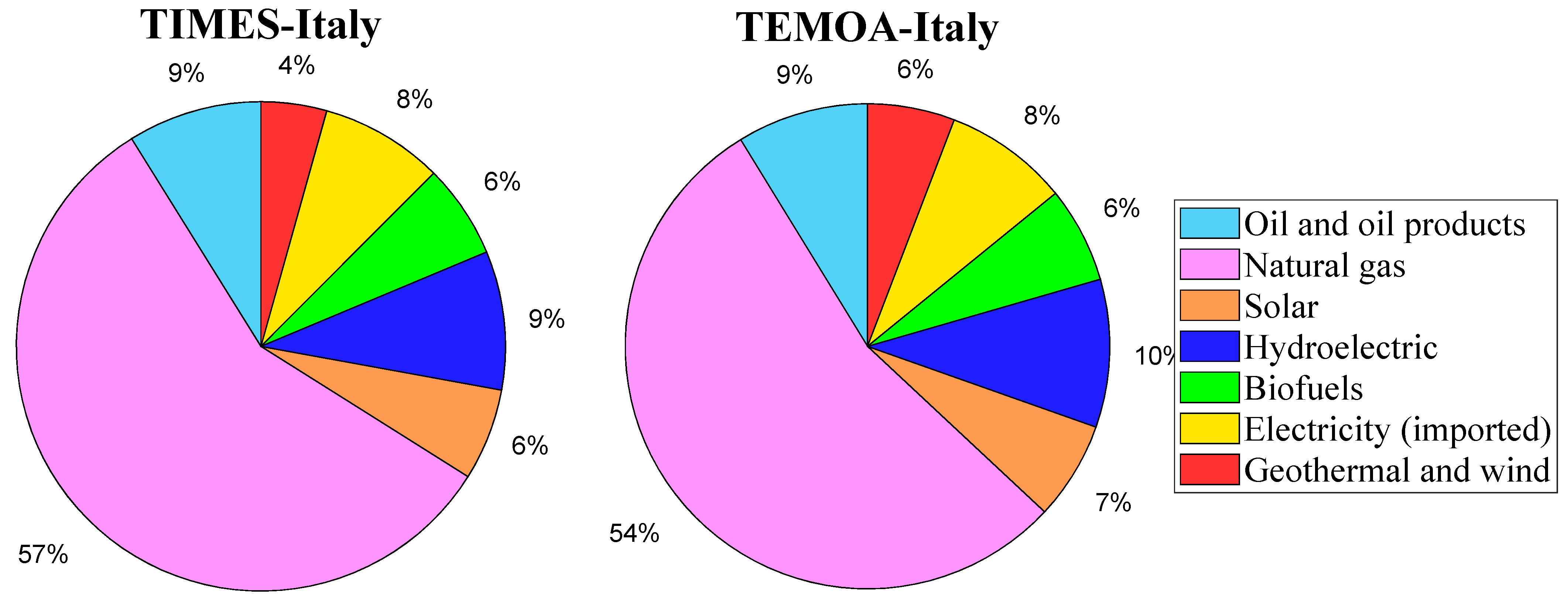
4.2. Aggregated Results
4.3. Disaggregated Results
- The contribution of each final technology to the production of each demand commodity and its evolution along the time horizon (technology mix).
- The consumption of each energy commodity, disaggregated by sector, and its contribution along the time horizon (energy mix).
- The associated costs to the selected technologies along the time horizon.
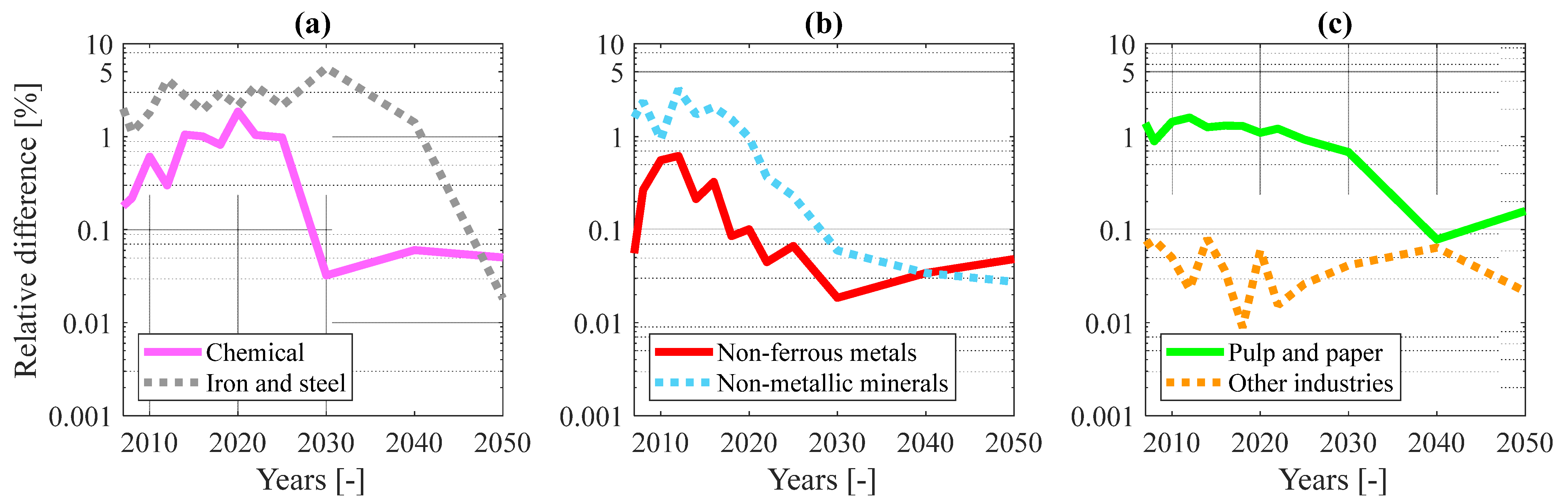
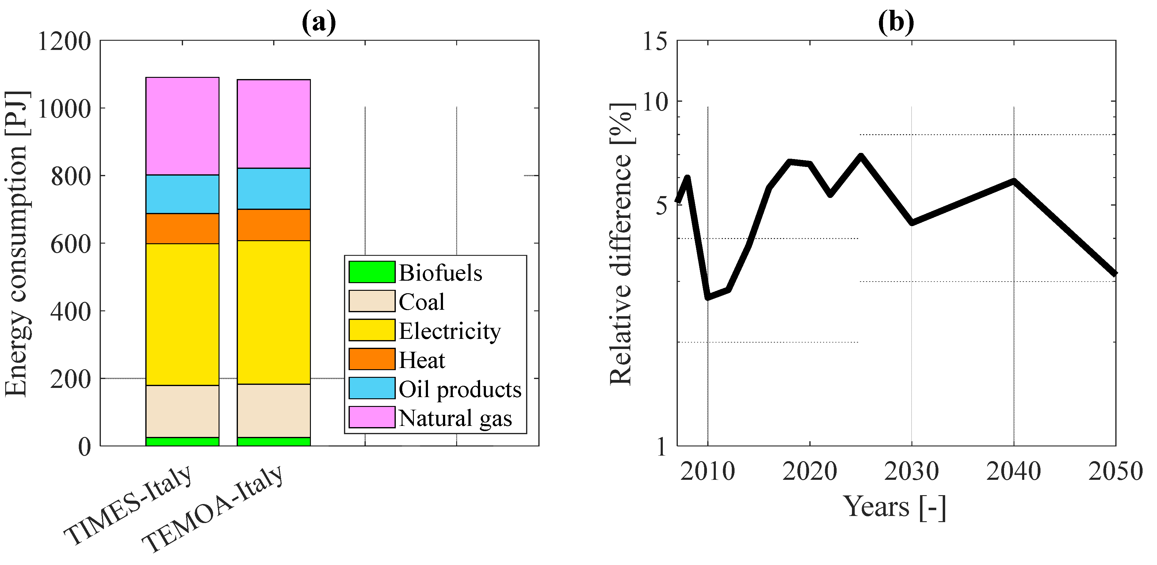
4.3.1. Industry
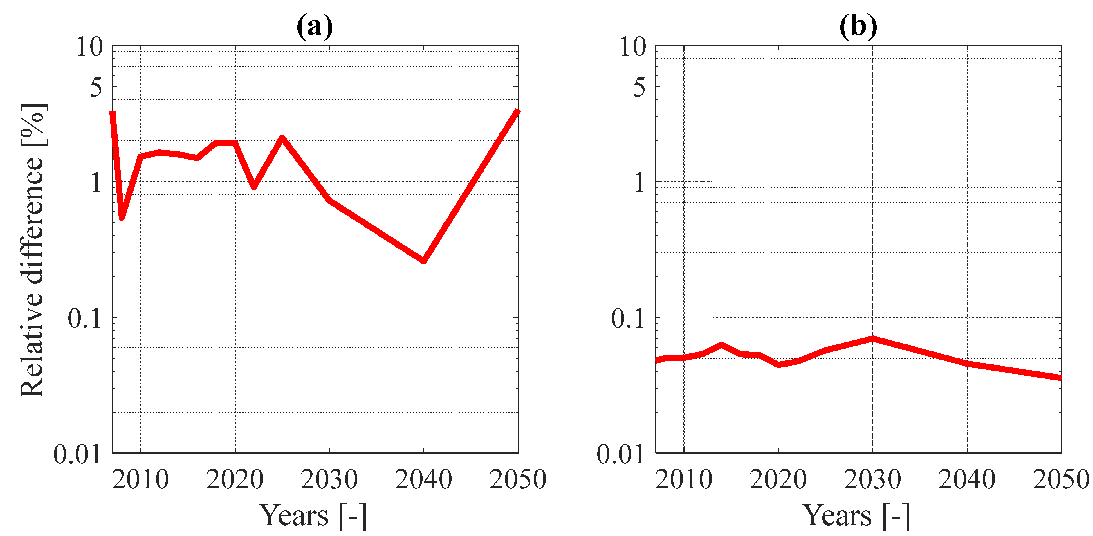
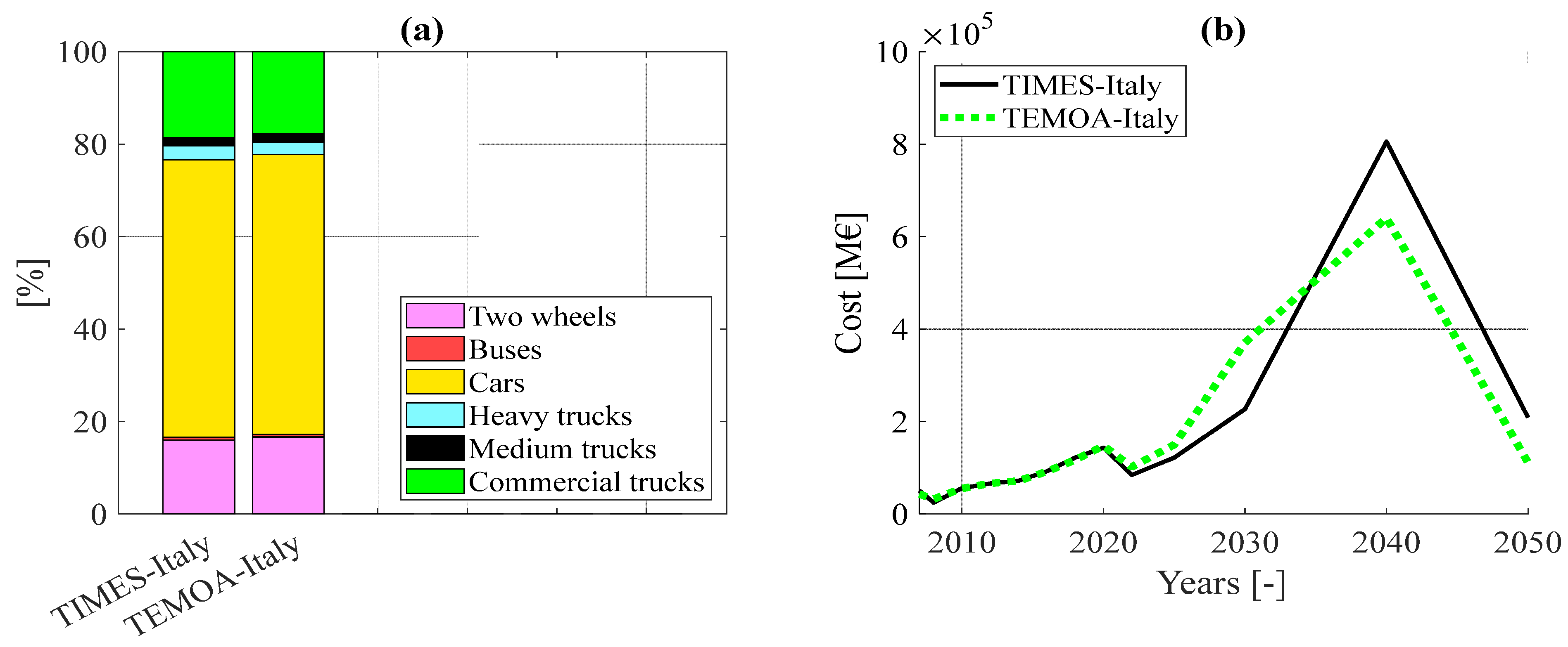
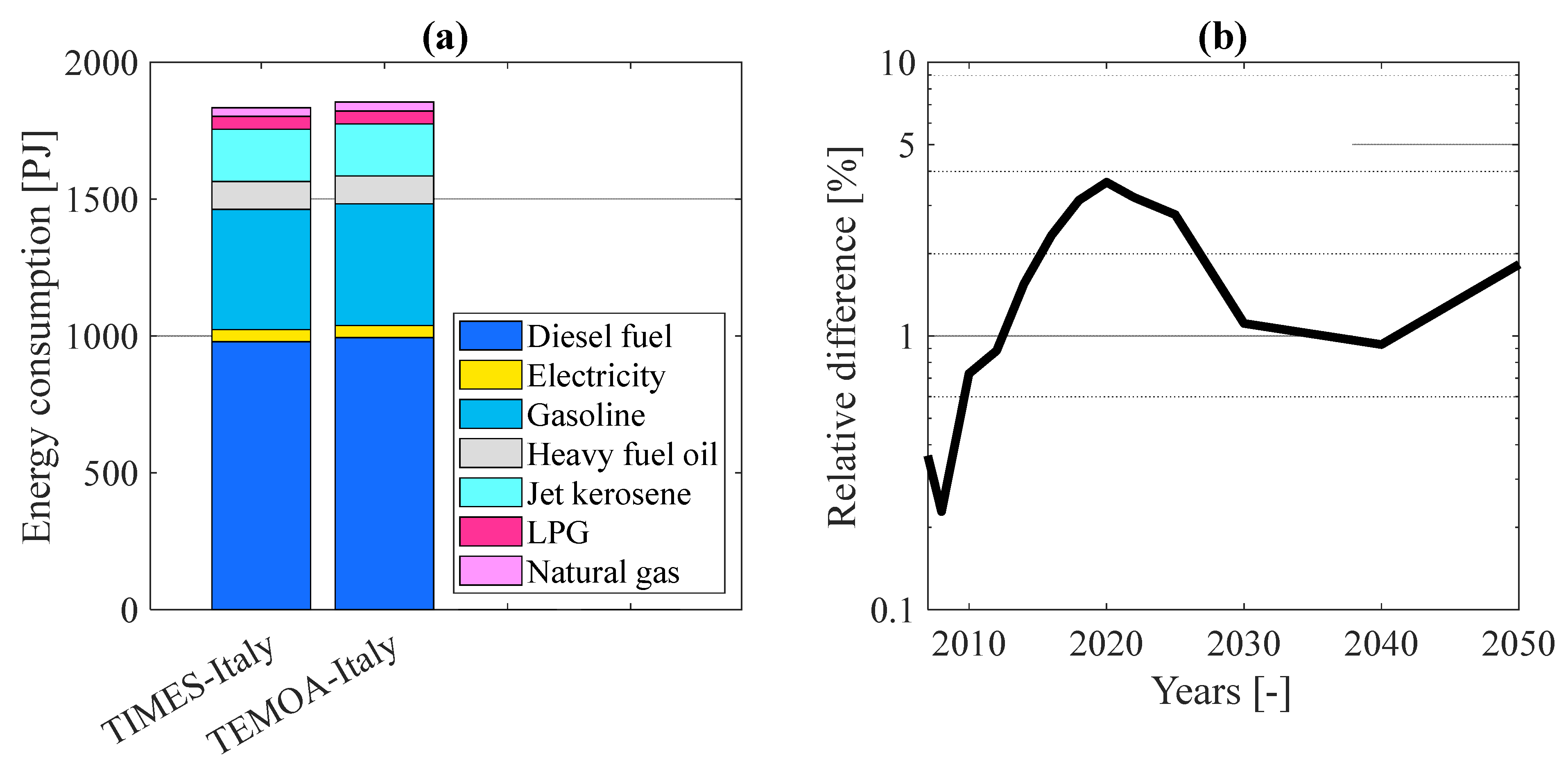
4.3.2. Transport
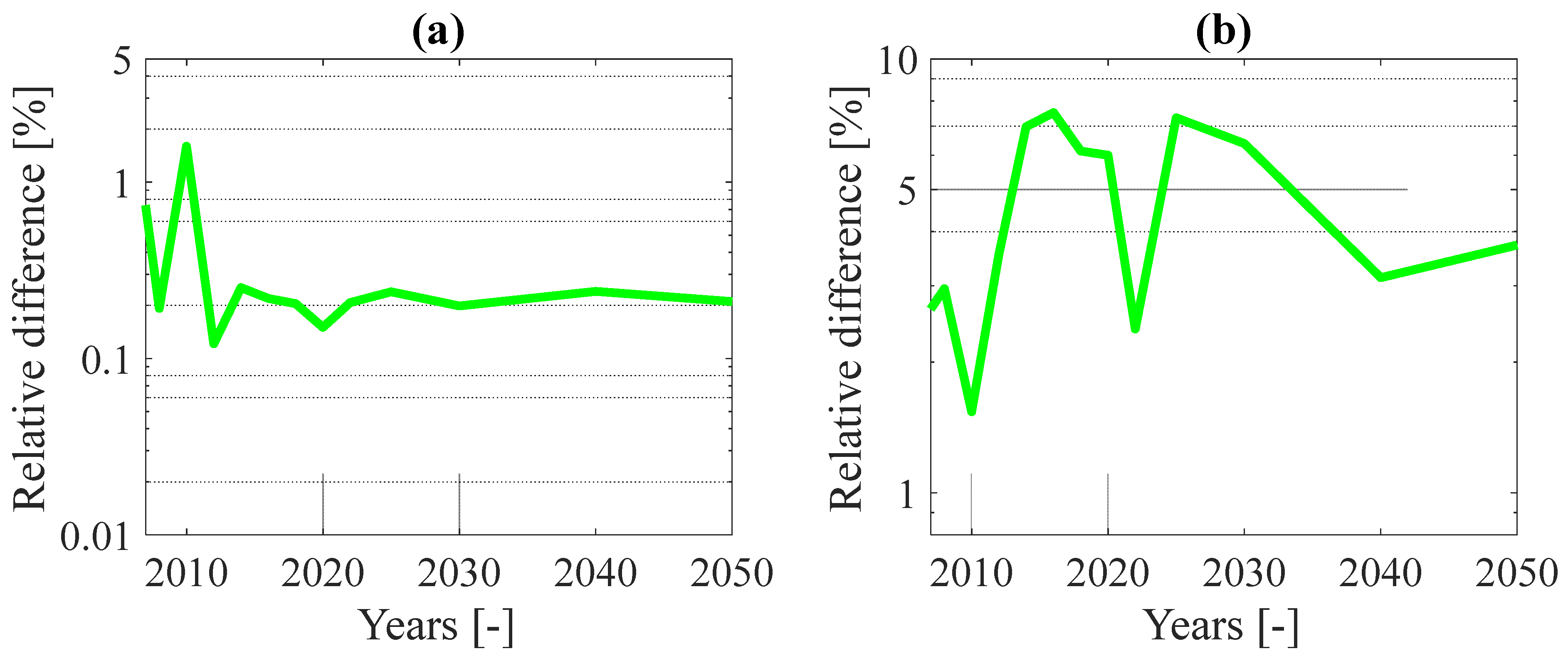
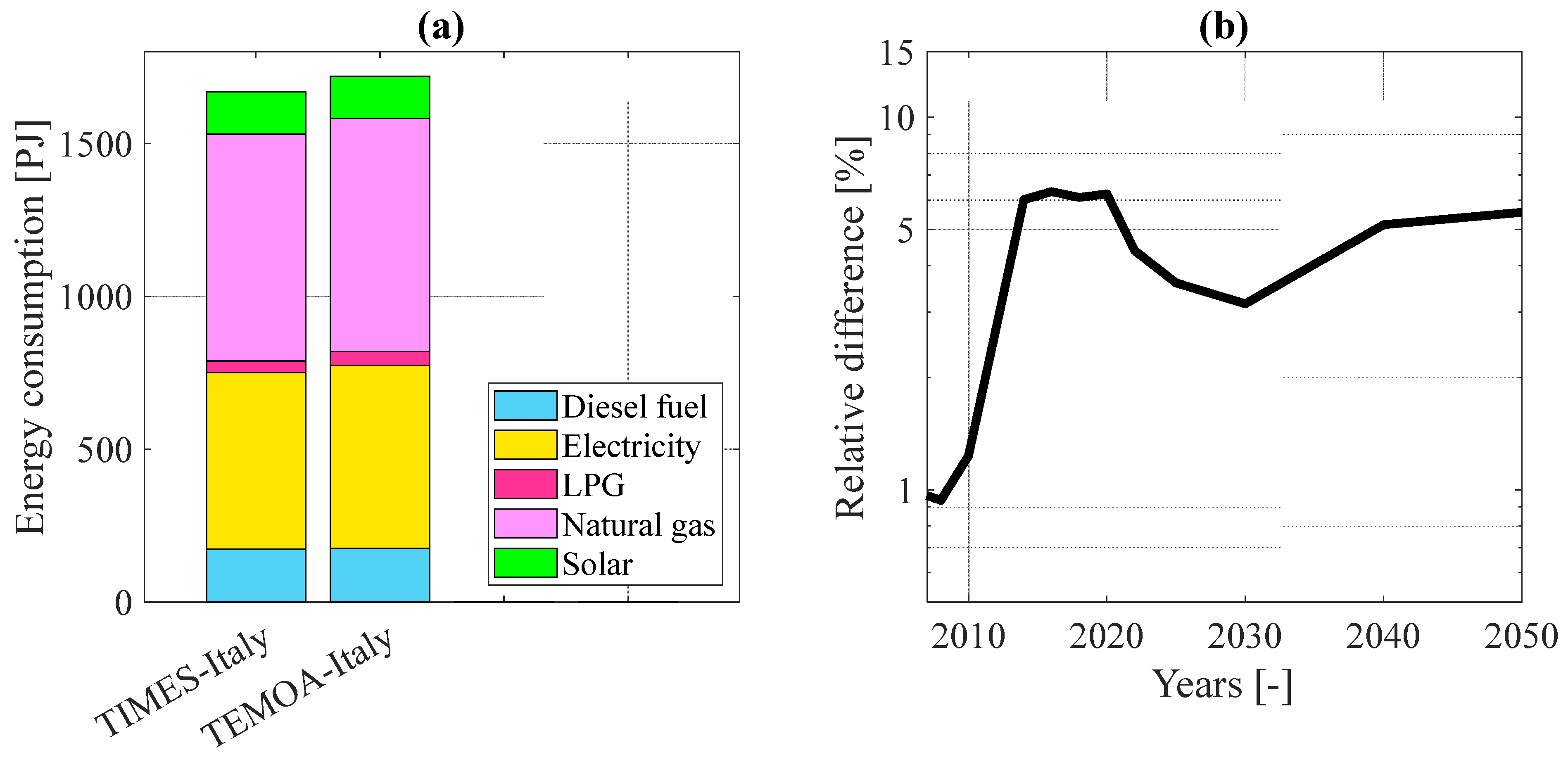
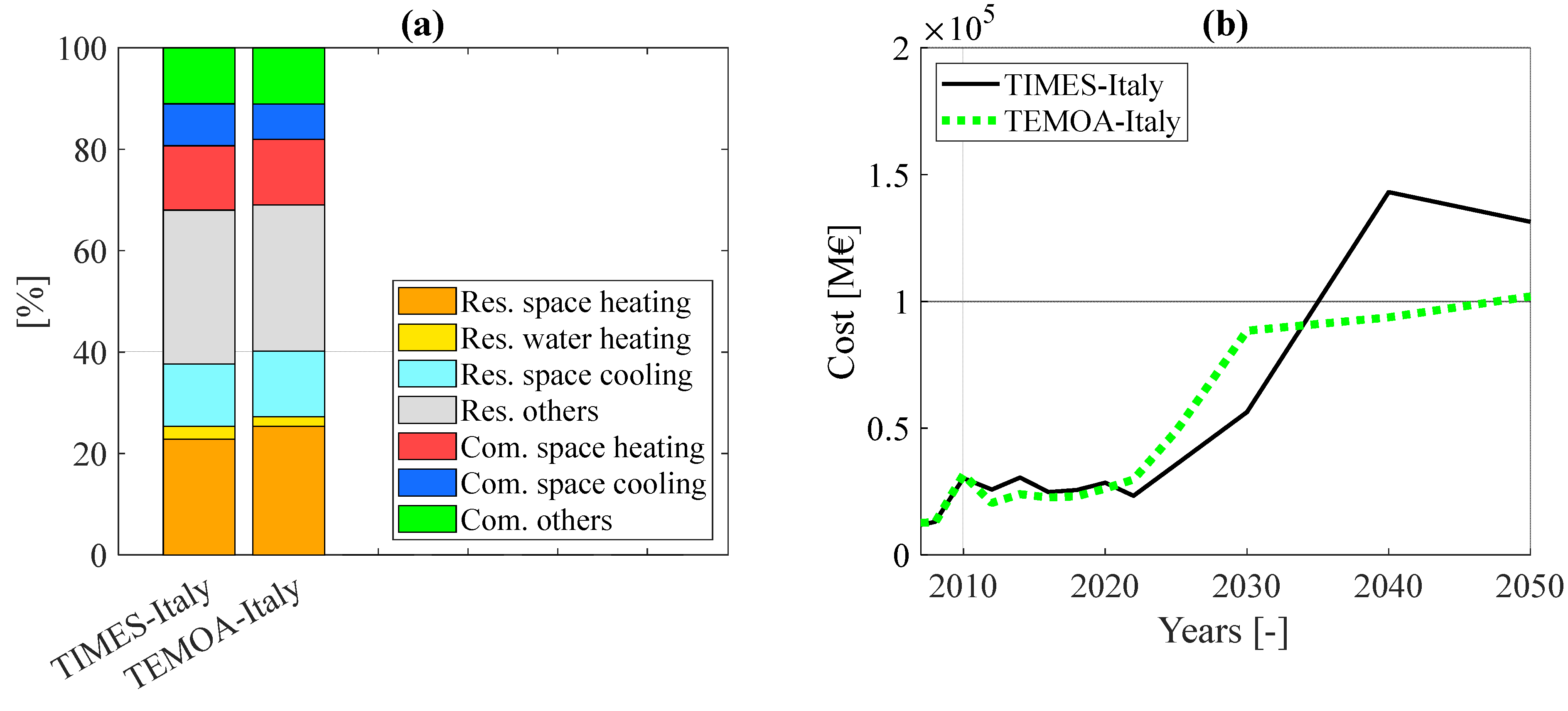
4.3.3. Buildings
5. Conclusions and Perspective
Author Contributions
Funding
Institutional Review Board Statement
Informed Consent Statement
Data Availability Statement
Acknowledgments
Conflicts of Interest
Appendix A. Enhancement of the TEMOA Framework
Appendix A.1. Description of the Technologies in the RES

- An automatic interpolation and extrapolation process (totally missing in the original TEMOA version [40], that requires the manual specification of the parameters for all the time periods included in the optimization process), performing the same operations encompassed in, e.g., the TIMES framework. This feature, including the option of setting different interpolation and extrapolation rules for different parameters in the Excel files, is automatically executed by the software. In particular, it is possible to assign interpolation/extrapolation options to the parameters included in the TEMOA database to set: (1) the interpolation type (linear or log-linear); (2) whether interpolation only or also extrapolation should be operated; and (3) whether extrapolation should be performed backward, forward, or both [54]. The most-common interpolation rule is the linear one, with constant extrapolation forward and, this is the general rule developed for the case-study presented here, with few exceptions. Table A1 lists the parameters for which interpolation and extrapolation are required, specifying the applied rule. Notably, the three main selected rules are: piecewise constant interpolation (implemented only for the lifetime parameter); piecewise linear interpolation (for all the parameters except for the lifetime); and constant extrapolation forward (for all the parameter except for constraint on technology groups’ activity). For the technology lifetime, a piecewise constant interpolation curve has been chosen, to maintain an integer value for the parameter. Note that the constraints applied to technology groups (rather than to single technologies) are only linearly interpolated, but not extrapolated forward, as it happens for the other parameters. It should be noted that a constant extrapolation forward could also be easily obtained for all the constraints on technology groups, simply repeating the last value of the interpolation in the last time step of the time horizon, without the necessity to change the preprocessing algorithm. This integration strongly simplifies the database construction and its modification, allowing the energy modeler to build databases representing large and complex RES.

| Parameter | Interpolation/Extrapolation Rule | ||
|---|---|---|---|
| Piecewise Constant Interpolation | Piecewise Linear Interpolation | Forward Constant Extrapolation | |
| LifetimeProcess | X | X | |
| Efficiency | X | X | |
| TechInputSplit | X | X | |
| TechOutputSplit | X | X | |
| EmissionActivity | X | X | |
| CostInvest | X | X | |
| CostFixed | X | X | |
| CostVariable | X | X | |
| MaxActivity | X | X | |
| MaxGenGroupLimit | X | ||
| MaxCapacity | X | X | |
| MinActivity | X | X | |
| MinGenGroupTarget | X | ||
| MinCapacity | X | X | |
| MaxInputGroup | X | ||
| MaxOutputGroup | X | ||
| MinInputGroup | X | ||
| CapacityFactor | X | X | |
| CapacityFactorProcess | X | X | |
| CapacityCredit | X | X | |
- The automatic evaluation of the technology-based emission factors, which are implemented in TEMOA through the dedicated parameter EmissionActivity, proportional to the technology activity. Being the EmissionActivity parameter indexed by region (index , emission commodity , input commodity , technology (index , year (index , and output commodity (index , the filling of the database would be very complex without an automatic computation of the emission factors. Furthermore, the emissions associated to the consumption of fossil fuels are usually equal for the same fuel (being dependent on its chemical composition). For that reason, a parameter representing the emission factors per unit of commodity consumed (CommodityEmissionFactor) has been added to the database, indexed by the input commodity to which the emission is associated and the emitted emission commodity. The operation performed in the preprocessing script (reported in Equation (A3)) is the sum of the contribution of the Commodity-based Emission Factor , divided by the efficiency of the technology to obtain the correspondent emission factor per unit of output, with the Technology-based Emission Factor (usually adopted to model process-related emissions) possibly manually inserted in the EmissionActivity table of the database, before being preprocessed. The output of the algorithm is the preprocessed database, with the complete EmissionActivity table.
Appendix A.2. Drivers for the Energy Service Demands
Appendix A.3. Constraints
Appendix A.4. The Optimization Problem
Appendix B. The Italian Energy System
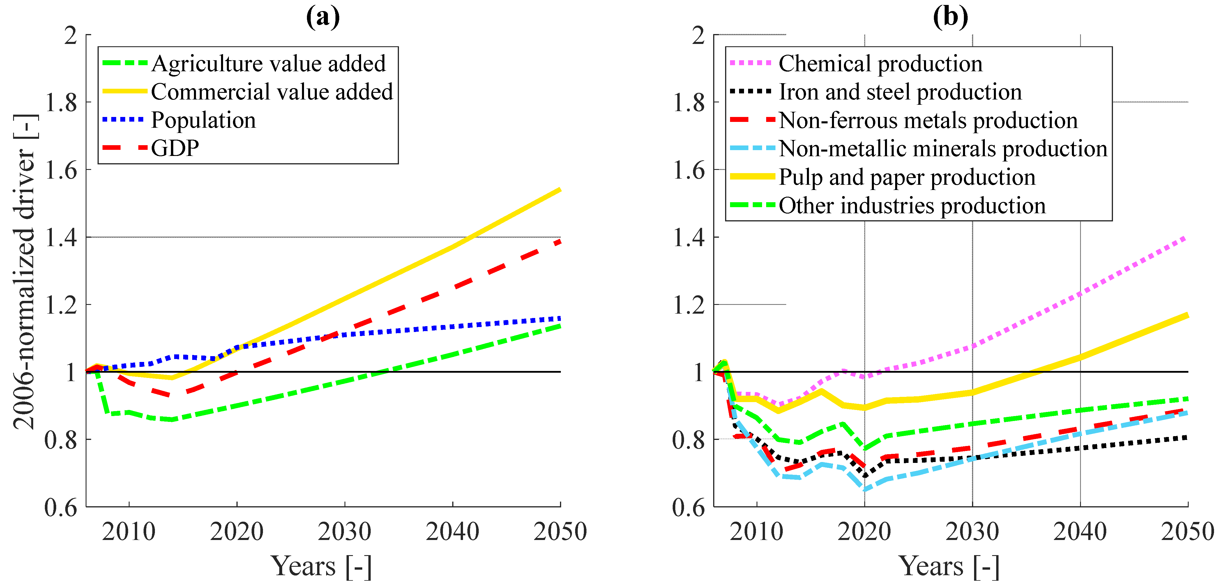
Appendix B.1. Drivers for Demand Projection in Future Years

Appendix B.2. Techno-Economic Characterization of the Main Demand-Side Subsectors
| Technology | Efficiency [PJ/Mt] | Availability Factor | Lifetime | Investment Cost [M€/cap.] | Fixed O&M Cost [M€/cap.] | ||
|---|---|---|---|---|---|---|---|
| Existing | Ammonia | 65.57 | 1.00 | 30 | - | - | |
| Chlorine | 12.85 | 1.00 | 30 | - | - | ||
| Aromatics | 73.21 | 1.00 | 30 | - | - | ||
| Olefins | 75.18 | 1.00 | 30 | - | - | ||
| Methanol | 48.86 | 1.00 | 30 | - | - | ||
| Other chemicals | 10.00 | 1.00 | 30 | - | - | ||
| New | Ammonia | Natural gas steam reforming | 46.08 | 0.90 | 25 | 860.00 | 21.50 |
| Naphtha POX | 48.31 | 0.90 | 25 | 1203.00 | 30.08 | ||
| Coal gasification | 45.76 | 0.90 | 25 | 2063.00 | 51.58 | ||
| Biomass gasification | 58.30 | 0.90 | 25 | 6000.00 | 300.00 | ||
| Electrolysis | 40.34 | 0.90 | 25 | 104.00 | 2.60 | ||
| Natural gas steam reforming with CCS | 45.52 | 0.90 | 25 | 930.00 | 51.00 | ||
| Chlorine | Mercury | 16.11 | 0.95 | 30 | 675.80 | 6.70 | |
| Diaphragm | 13.05 | 0.95 | 30 | 675.80 | 6.70 | ||
| Membrane | 12.33 | 0.95 | 30 | 675.80 | 6.70 | ||
| Methanol | Natural gas steam reforming | 37.90 | 0.85 | 25 | 295.00 | 21.50 | |
| COG steam reforming | 52.50 | 0.85 | 30 | 295.00 | 21.50 | ||
| LPG steam reforming | 37.80 | 0.85 | 30 | 295.00 | 21.50 | ||
| Coal gasification | 50.10 | 0.85 | 30 | 710.00 | 17.75 | ||
| Biomass gasification | 61.40 | 0.85 | 30 | 4900.00 | 245.00 | ||
| Electrolysis | 23.90 | 0.95 | 30 | 44.00 | 1.10 | ||
| HVC | Naphtha steam cracking | 94.20 | 0.90 | 30 | 2057.00 | 51.40 | |
| Ethane steam cracking | 70.60 | 0.85 | 30 | 1487.00 | 37.20 | ||
| Gas oil steam cracking | 102.20 | 0.85 | 30 | 2328.00 | 58.20 | ||
| LPG steam cracking | 93.00 | 0.85 | 30 | 1900.00 | 47.50 | ||
| Naphtha catalytic cracking | 74.10 | 0.85 | 30 | 3000.00 | 75.00 | ||
| Bioethanol dehydration | 94.90 | 0.85 | 30 | 1328.00 | 33.20 | ||
| Olefins | Prophane dehydrogenation | 69.40 | 0.85 | 30 | 1691.00 | 42.30 | |
| Methanol-to-olefins | 65.77 | 0.85 | 30 | 1000.00 | 25.00 | ||
| Technology | Efficiency [Bvkm/PJ] | Availability Factor | Lifetime | Investment Cost [M€/cap.] | Fixed O&M Cost [M€/cap.] | |
|---|---|---|---|---|---|---|
| Existing | Gasoline car | 0.30 | 1.00 | 12 | - | - |
| Diesel car | 0.36 | 1.00 | 12 | - | - | |
| LPG car | 0.25 | 1.00 | 12 | - | - | |
| Natural gas car | 0.27 | 1.00 | 12 | - | - | |
| Biofuels car | 0.44 | 1.00 | 12 | - | - | |
| New | Gasoline car | 0.31 ÷ 0.41 | 1.00 | 12 | 1000.00 | 62.63 |
| Diesel car | 0.38 ÷ 0.50 | 1.00 | 12 | 1081.78 | 62.63 | |
| LPG car | 0.34 | 1.00 | 12 | 1081.78 | 64.37 | |
| Natural gas car | 0.36 | 1.00 | 12 | 1081.78 | 64.37 | |
| Electric car | 1.18 ÷ 1.37 | 1.00 | 12 | 2202.34 ÷ 1262.66 | 51.33 | |
| Hybrid electric car | 0.45 ÷ 0.69 | 1.00 | 12 | 1284.14 ÷ 1140.63 | 61.76 | |
| Fuel cell car | 0.64 ÷ 0.94 | 1.00 | 12 | 4328.62 ÷ 1814.60 | 70.03 ÷ 60.89 | |
| Technology | Efficiency [PJu/PJf] | Availability Factor | Lifetime | Investment Cost [M€/cap.] | Fixed O&M Cost [M€/cap.] | |
|---|---|---|---|---|---|---|
| Existing | Natural gas boiler | 0.73 | 0.18 | 20 | - | - |
| Diesel fuel boiler | 0.73 | 0.18 | 20 | - | - | |
| LPG boiler | 0.68 | 0.18 | 20 | - | - | |
| Wood stove | 0.25 | 0.18 | 20 | - | - | |
| Heat exchanger | 0.90 | 0.18 | 20 | - | - | |
| New | Diesel fuel boiler | 0.81 | 1.00 | 20 | 5.87 | 0.06 |
| Condensing diesel fuel boiler | 0.90 ÷ 0.98 | 1.00 | 20 | 8.72 | 0.09 | |
| Solar and diesel fuel boiler | 0.82 ÷ 0.90 | 1.00 | 20 | 23.50 ÷ 21.48 | 0.07 | |
| Natural gas boiler | 0.78 ÷ 0.90 | 1.00 | 20 | 4.99 | 0.05 | |
| Condensing natural gas boiler | 0.85 ÷ 0.98 | 1.00 | 20 | 6.84 | 0.07 | |
| Solar and natural gas boiler | 0.82 ÷ 0.90 | 1.00 | 20 | 22.40 ÷ 20.56 | 0.06 | |
| LPG boiler | 0.81 | 1.00 | 20 | 5.47 | 0.05 | |
| Condensing LPG boiler | 0.90 ÷ 0.98 | 1.00 | 20 | 7.00 | 0.07 | |
| Solar and LPG boiler | 0.82 ÷ 0.90 | 1.00 | 20 | 23.00 ÷ 21.02 | 0.06 | |
| Wood stove | 0.50 | 1.00 | 20 | 2.00 | 0.02 | |
| Wood pellet stove | 0.76 ÷ 0.83 | 1.00 | 20 | 15.85 | 0.16 | |
| Electric heat pumps | 3.30 ÷ 5.75 | 1.00 | 20 ÷ 50 | 47.56 ÷ 66.59 | 0.48 ÷ 0.67 | |
| Multipurpose heat pump | 3.30 ÷ 4.71 | 0.40 | 20 | 47.56 | 0.48 | |
| Heat exchanger | 0.90 | 1.00 | 20 | 2.88 | 0.03 | |
| Insulation | - | - | 20 ÷ 50 | 481.32 ÷ 2767.65 | - | |
Appendix C. Detailed Results Comparison of Final Technologies Belonging to the Demand-Side Sectors
| Subsector | Technology | Model | Process Activity [Mt] | Cumulative Activity [Mt] | diffcum [%] | ||||||||||||
|---|---|---|---|---|---|---|---|---|---|---|---|---|---|---|---|---|---|
| Year | |||||||||||||||||
| 2007 | 2008 | 2010 | 2012 | 2014 | 2016 | 2018 | 2020 | 2022 | 2025 | 2030 | 2040 | 2050 | |||||
| Chemical | Ammonia existing | TIMES-Italy | 0.62 | 0.58 | 0.50 | 0.44 | 0.37 | 0.30 | 0.24 | 0.17 | 0.10 | 6.11 | 0.31 | ||||
| TEMOA-Italy | 0.62 | 0.57 | 0.50 | 0.44 | 0.37 | 0.30 | 0.24 | 0.17 | 0.10 | 6.10 | |||||||
| Ammonia naphtha POX | TIMES-Italy | 0.09 | 0.14 | 0.14 | 0.14 | 0.14 | 0.14 | 0.14 | 0.14 | 2.69 | |||||||
| TEMOA-Italy | 0.02 | 0.02 | 0.09 | 0.14 | 0.21 | 0.21 | 0.20 | 0.00 | 0.20 | 0.19 | 3.30 | ||||||
| Ammonia natural gas steam reforming | TIMES-Italy | 0.02 | 0.02 | 0.08 | 0.18 | 0.27 | 0.32 | 0.40 | 0.52 | 0.69 | 0.79 | 0.90 | 22.94 | ||||
| TEMOA-Italy | 0.00 | 0.00 | 0.01 | 0.11 | 0.20 | 0.46 | 0.35 | 0.46 | 0.69 | 0.79 | 0.89 | 22.30 | |||||
| Chlorine existing | TIMES-Italy | 0.20 | 0.19 | 0.18 | 0.16 | 0.14 | 0.13 | 0.09 | 0.09 | 0.07 | 0.04 | 2.61 | |||||
| TEMOA-Italy | 0.20 | 0.19 | 0.17 | 0.15 | 0.12 | 0.10 | 0.08 | 0.06 | 0.03 | 0.00 | 2.03 | ||||||
| Chlorine membrane | TIMES-Italy | 0.01 | 0.01 | 0.02 | 0.03 | 0.05 | 0.08 | 0.12 | 0.12 | 0.14 | 0.17 | 0.23 | 0.26 | 0.30 | 7.97 | ||
| TEMOA-Italy | 0.01 | 0.01 | 0.03 | 0.05 | 0.07 | 0.11 | 0.14 | 0.15 | 0.18 | 0.22 | 0.23 | 0.26 | 0.30 | 8.57 | |||
| Aromatics existing | TIMES-Italy | 0.77 | 0.74 | 0.63 | 0.60 | 0.54 | 0.47 | 0.40 | 0.34 | 0.27 | 0.17 | 9.86 | |||||
| TEMOA-Italy | 0.77 | 0.74 | 0.63 | 0.60 | 0.54 | 0.47 | 0.40 | 0.34 | 0.27 | 0.17 | 9.86 | ||||||
| Olefins existing | TIMES-Italy | 2.84 | 2.64 | 2.43 | 2.22 | 1.98 | 1.73 | 1.48 | 1.24 | 0.99 | 0.62 | 36.33 | |||||
| TEMOA-Italy | 2.84 | 2.64 | 2.38 | 2.22 | 1.98 | 1.73 | 1.48 | 1.23 | 0.99 | 0.62 | 36.21 | ||||||
| HVC gas oil steam cracking | TIMES-Italy | 0.11 | 0.11 | 0.42 | 0.54 | 0.93 | 1.43 | 1.86 | 2.10 | 2.50 | 3.05 | 4.01 | 4.60 | 5.23 | 139.46 | ||
| TEMOA-Italy | 0.12 | 0.12 | 0.47 | 0.55 | 0.92 | 1.43 | 1.86 | 2.11 | 2.51 | 3.05 | 4.02 | 4.60 | 5.24 | 139.71 | |||
| Methanol existing | TIMES-Italy | 0.05 | 0.05 | 0.04 | 0.04 | 0.03 | 0.02 | 0.02 | 0.01 | 0.01 | 0.49 | ||||||
| TEMOA-Italy | 0.05 | 0.04 | 0.04 | 0.04 | 0.03 | 0.02 | 0.02 | 0.01 | 0.01 | 0.49 | |||||||
| Methanol natural gas steam reforming | TIMES-Italy | 0.00 | 0.00 | 0.00 | 0.01 | 0.02 | 0.02 | 0.03 | 0.04 | 0.04 | 0.05 | 0.05 | 0.06 | 0.07 | 1.96 | ||
| TEMOA-Italy | 0.00 | 0.00 | 0.00 | 0.01 | 0.01 | 0.02 | 0.03 | 0.04 | 0.04 | 0.05 | 0.05 | 0.06 | 0.07 | 1.98 | |||
| Other chemicals | TIMES-Italy | 16.02 | 15.01 | 14.97 | 14.49 | 14.79 | 15.60 | 16.11 | 15.79 | 16.16 | 16.47 | 17.26 | 19.78 | 22.51 | 798.30 | ||
| TEMOA-Italy | 16.02 | 15.02 | 14.97 | 14.50 | 14.79 | 15.61 | 16.11 | 15.81 | 16.18 | 16.48 | 17.27 | 19.79 | 22.52 | 798.69 | |||
| Iron and steel | Basic oxygen furnace existing | TIMES-Italy | 11.33 | 9.48 | 8.39 | 6.83 | 6.08 | 5.63 | 4.74 | 3.70 | 3.54 | 2.46 | 123.95 | 2.57 | |||
| TEMOA-Italy | 11.30 | 9.63 | 8.62 | 7.27 | 6.39 | 5.81 | 5.10 | 3.92 | 3.94 | 2.46 | 128.90 | ||||||
| Basic oxygen furnace new | TIMES-Italy | 0.65 | 0.23 | 0.44 | 0.31 | 0.18 | 0.36 | 0.24 | 0.65 | 0.65 | 0.65 | 0.17 | 17.57 | ||||
| TEMOA-Italy | 0.96 | 0.00 | 0.00 | 0.00 | 0.00 | 0.00 | 0.02 | 0.25 | 0.41 | 0.00 | 0.00 | 3.79 | |||||
| HIsarna process | TIMES-Italy | 1.09 | 3.59 | 4.23 | 4.59 | 97.44 | |||||||||||
| TEMOA-Italy | 1.33 | 4.24 | 4.41 | 4.59 | 106.90 | ||||||||||||
| Electric arc furnace existing | TIMES-Italy | 18.98 | 17.08 | 16.50 | 14.85 | 13.20 | 11.55 | 9.90 | 8.25 | 6.60 | 4.13 | 242.09 | |||||
| TEMOA-Italy | 19.00 | 16.94 | 16.50 | 14.90 | 13.20 | 11.60 | 9.90 | 8.25 | 6.60 | 4.13 | 242.03 | ||||||
| Electric arc furnace new | TIMES-Italy | 1.83 | 0.22 | 1.48 | 3.55 | 6.45 | 9.04 | 9.69 | 12.47 | 15.00 | 19.32 | 20.07 | 20.91 | 631.74 | |||
| TEMOA-Italy | 1.54 | 0.22 | 1.43 | 3.57 | 6.41 | 9.04 | 9.70 | 12.49 | 15.01 | 19.32 | 20.07 | 20.90 | 631.43 | ||||
| Non-ferrous metals | Aluminum existing | TIMES-Italy | 2.03 | 1.68 | 1.66 | 1.43 | 1.41 | 1.24 | 1.06 | 0.88 | 0.71 | 0.44 | 25.09 | 0.07 | |||
| TEMOA-Italy | 2.03 | 1.68 | 1.66 | 1.43 | 1.41 | 1.24 | 1.06 | 0.88 | 0.71 | 0.44 | 25.08 | ||||||
| Aluminum new | TIMES-Italy | 0.05 | 0.01 | 0.05 | 0.05 | 0.11 | 0.36 | 0.56 | 0.63 | 0.86 | 1.14 | 1.63 | 1.75 | 1.86 | 51.18 | ||
| TEMOA-Italy | 0.05 | 0.02 | 0.05 | 0.05 | 0.11 | 0.36 | 0.56 | 0.63 | 0.86 | 1.14 | 1.63 | 1.75 | 1.86 | 51.18 | |||
| Copper existing | TIMES-Italy | 0.38 | 0.32 | 0.31 | 0.27 | 0.27 | 0.23 | 0.20 | 0.17 | 0.13 | 0.08 | 4.72 | |||||
| TEMOA-Italy | 0.38 | 0.32 | 0.31 | 0.27 | 0.27 | 0.23 | 0.20 | 0.17 | 0.13 | 0.08 | 4.72 | ||||||
| Copper new | TIMES-Italy | 0.01 | 0.00 | 0.01 | 0.01 | 0.02 | 0.07 | 0.11 | 0.12 | 0.16 | 0.22 | 0.31 | 0.33 | 0.35 | 9.64 | ||
| TEMOA-Italy | 0.01 | 0.00 | 0.01 | 0.01 | 0.02 | 0.07 | 0.11 | 0.12 | 0.16 | 0.22 | 0.31 | 0.33 | 0.35 | 9.63 | |||
| Other non-ferrous metals | TIMES-Italy | 1.40 | 1.14 | 1.14 | 0.99 | 1.02 | 1.07 | 1.09 | 1.01 | 1.05 | 1.06 | 1.09 | 1.17 | 1.25 | 51.23 | ||
| TEMOA-Italy | 1.40 | 1.14 | 1.14 | 0.99 | 1.02 | 1.07 | 1.09 | 1.01 | 1.06 | 1.06 | 1.09 | 1.17 | 1.25 | 51.21 | |||
| Zinc existing | TIMES-Italy | 0.36 | 0.30 | 0.30 | 0.26 | 0.25 | 0.22 | 0.19 | 0.16 | 0.13 | 0.08 | 4.51 | |||||
| TEMOA-Italy | 0.37 | 0.31 | 0.31 | 0.27 | 0.25 | 0.22 | 0.19 | 0.16 | 0.13 | 0.08 | 4.55 | ||||||
| Zinc new | TIMES-Italy | 0.01 | 0.01 | 0.01 | 0.02 | 0.06 | 0.10 | 0.11 | 0.16 | 0.21 | 0.29 | 0.31 | 0.33 | 9.19 | |||
| TEMOA-Italy | 0.01 | 0.00 | 0.00 | 0.02 | 0.06 | 0.10 | 0.11 | 0.16 | 0.21 | 0.29 | 0.31 | 0.33 | 9.15 | ||||
| Non-metallic minerals | Dry cement kilns existing | TIMES-Italy | 33.14 | 29.10 | 26.88 | 22.25 | 22.81 | 20.17 | 17.29 | 14.41 | 11.53 | 7.20 | 409.53 | 0.35 | |||
| TEMOA-Italy | 33.10 | 29.58 | 25.70 | 24.20 | 23.00 | 20.10 | 17.30 | 14.40 | 11.50 | 7.20 | 412.16 | ||||||
| Wet cement kilns existing | TIMES-Italy | 13.21 | 11.60 | 10.23 | 8.87 | 7.51 | 8.04 | 6.89 | 5.74 | 4.59 | 2.87 | 159.11 | |||||
| TEMOA-Italy | 13.20 | 11.60 | 11.40 | 8.88 | 7.52 | 8.03 | 6.89 | 5.74 | 4.59 | 2.87 | 161.45 | ||||||
| Blended cement new | TIMES-Italy | 2.57 | 0.49 | 1.95 | 2.57 | 6.55 | 10.08 | 11.02 | 16.51 | 23.47 | 35.54 | 39.10 | 42.09 | 1107.47 | |||
| TEMOA-Italy | 2.63 | 0.00 | 0.00 | 2.37 | 6.63 | 10.09 | 11.03 | 16.57 | 23.50 | 35.52 | 39.12 | 42.08 | 1102.73 | ||||
| Dry clinker new | TIMES-Italy | 1.70 | 0.32 | 1.28 | 1.70 | 4.32 | 6.65 | 7.27 | 10.90 | 15.49 | 23.46 | 25.81 | 27.78 | 730.93 | |||
| TEMOA-Italy | 1.74 | 0.00 | 0.00 | 1.57 | 4.38 | 6.66 | 7.28 | 10.93 | 15.51 | 23.45 | 25.82 | 27.77 | 727.80 | ||||
| Bricks existing | TIMES-Italy | 5.88 | 5.17 | 4.56 | 3.95 | 3.34 | 2.74 | 2.13 | 1.52 | 0.91 | 55.44 | ||||||
| TEMOA-Italy | 5.47 | 5.17 | 4.56 | 3.95 | 3.34 | 2.73 | 2.13 | 1.52 | 0.91 | 55.01 | |||||||
| Bricks new | TIMES-Italy | 0.33 | 0.06 | 0.15 | 0.25 | 0.83 | 1.68 | 2.22 | 2.44 | 3.23 | 4.26 | 4.51 | 4.97 | 5.35 | 157.40 | ||
| TEMOA-Italy | 0.74 | 0.06 | 0.15 | 0.25 | 0.84 | 1.68 | 2.22 | 2.44 | 3.23 | 4.26 | 4.51 | 4.97 | 5.34 | 157.81 | |||
| Glass existing | TIMES-Italy | 3.52 | 3.13 | 2.73 | 2.51 | 2.45 | 1.99 | 1.70 | 1.45 | 1.22 | 0.77 | 42.93 | |||||
| TEMOA-Italy | 3.52 | 3.13 | 2.75 | 2.52 | 2.30 | 2.14 | 1.84 | 1.53 | 1.21 | 0.77 | 43.39 | ||||||
| Glass new | TIMES-Italy | 0.20 | 0.09 | 0.05 | 0.66 | 0.90 | 0.92 | 1.26 | 1.78 | 2.70 | 2.97 | 3.20 | 84.49 | ||||
| TEMOA-Italy | 0.12 | 0.00 | 0.12 | 0.43 | 0.69 | 0.77 | 1.19 | 1.71 | 2.69 | 2.98 | 3.20 | 82.50 | |||||
| Lime existing | TIMES-Italy | 5.02 | 4.41 | 4.02 | 3.37 | 3.29 | 3.06 | 2.62 | 2.18 | 1.75 | 1.09 | 61.64 | |||||
| TEMOA-Italy | 5.02 | 4.41 | 4.02 | 3.40 | 3.28 | 2.84 | 2.42 | 2.08 | 1.75 | 1.09 | 60.63 | ||||||
| Lime new | TIMES-Italy | 0.28 | 0.05 | 0.21 | 0.28 | 0.71 | 1.09 | 1.19 | 1.79 | 2.54 | 3.85 | 4.24 | 4.56 | 120.05 | |||
| TEMOA-Italy | 0.29 | 0.06 | 0.19 | 0.29 | 0.93 | 1.30 | 1.30 | 1.79 | 2.55 | 3.85 | 4.24 | 4.56 | 121.18 | ||||
| Pulp and paper | Paper mill existing | TIMES-Italy | 9.59 | 8.90 | 8.34 | 7.51 | 6.67 | 5.84 | 5.00 | 4.17 | 3.34 | 2.09 | 122.89 | 0.65 | |||
| TEMOA-Italy | 9.59 | 8.95 | 8.34 | 7.51 | 6.67 | 5.84 | 5.00 | 4.17 | 3.34 | 2.08 | 122.97 | ||||||
| Paper mill new | TIMES-Italy | 0.71 | 0.31 | 0.87 | 1.35 | 2.45 | 3.59 | 4.01 | 4.77 | 5.82 | 7.11 | 9.40 | 10.44 | 11.71 | 321.81 | ||
| TEMOA-Italy | 0.71 | 0.26 | 0.87 | 1.34 | 2.45 | 3.59 | 4.02 | 4.78 | 5.82 | 7.11 | 9.40 | 10.44 | 11.71 | 321.84 | |||
| Chemical pulp existing | TIMES-Italy | 0.15 | 0.14 | 0.13 | 0.12 | 0.10 | 0.09 | 0.08 | 0.06 | 0.05 | 0.03 | 1.90 | |||||
| TEMOA-Italy | 0.15 | 0.14 | 0.13 | 0.12 | 0.09 | 0.07 | 0.06 | 0.04 | 0.02 | 0.00 | 1.90 | ||||||
| Chemical pulp new | TIMES-Italy | 0.01 | 0.01 | 0.01 | 0.03 | 0.04 | 0.05 | 0.06 | 0.07 | 0.08 | 0.11 | 0.11 | 0.12 | 3.61 | |||
| TEMOA-Italy | 0.01 | 0.00 | 0.01 | 0.01 | 0.03 | 0.04 | 0.05 | 0.06 | 0.07 | 0.09 | 0.11 | 0.11 | 0.12 | 3.62 | |||
| Mechanical pulp existing | TIMES-Italy | 0.33 | 0.32 | 0.29 | 0.26 | 0.23 | 0.20 | 0.17 | 0.14 | 0.12 | 0.07 | 4.29 | |||||
| TEMOA-Italy | 0.37 | 0.35 | 0.30 | 0.26 | 0.22 | 0.18 | 0.14 | 0.10 | 0.06 | 0.00 | 3.67 | ||||||
| Mechanical pulp new | TIMES-Italy | 0.04 | 0.04 | 0.04 | 0.07 | 0.10 | 0.11 | 0.13 | 0.16 | 0.19 | 0.25 | 0.26 | 0.27 | 8.28 | |||
| TEMOA-Italy | 0.00 | 0.00 | 0.01 | 0.01 | 0.04 | 0.08 | 0.09 | 0.12 | 0.15 | 0.19 | 0.25 | 0.26 | 0.27 | 8.01 | |||
| Recycled pulp existing | TIMES-Italy | 5.35 | 5.10 | 4.65 | 4.18 | 3.72 | 3.25 | 2.79 | 2.32 | 1.86 | 1.16 | 68.77 | |||||
| TEMOA-Italy | 5.28 | 5.11 | 4.59 | 4.12 | 3.67 | 3.20 | 2.75 | 2.31 | 1.84 | 1.16 | 68.10 | ||||||
| Recycled pulp new | TIMES-Italy | 0.35 | 0.43 | 0.69 | 1.25 | 1.82 | 2.02 | 2.38 | 2.88 | 3.48 | 4.52 | 5.04 | 5.67 | 156.13 | |||
| TEMOA-Italy | 0.44 | 0.00 | 0.54 | 0.79 | 1.34 | 1.92 | 2.12 | 2.49 | 3.01 | 3.59 | 4.60 | 5.03 | 5.65 | 159.09 | |||
| Other industries | Other industries existing | TIMES-Italy | 487.4 | 425.8 | 409.3 | 384.8 | 381.5 | 405.1 | 416.3 | 380.1 | 394.0 | 399.1 | 407.2 | 416.9 | 424.9 | 18,785.8 | 0.02 |
| TEMOA-Italy | 487.7 | 426.1 | 409.5 | 384.9 | 381.8 | 405.0 | 416.3 | 379.9 | 393.9 | 399.0 | 407.0 | 416.6 | 424.8 | 18,781.8 | |||
| Technology | Model | Process Activity [Bvkm] | Cumulative Activity [Bvkm] | diffcum [%] | ||||||||||||
|---|---|---|---|---|---|---|---|---|---|---|---|---|---|---|---|---|
| Year | ||||||||||||||||
| 2007 | 2008 | 2010 | 2012 | 2014 | 2016 | 2018 | 2020 | 2022 | 2025 | 2030 | 2040 | 2050 | ||||
| Biofuels existing | TIMES-Italy | 0.78 | 0.75 | 0.62 | 0.50 | 0.37 | 0.25 | 0.12 | 6.00 | 0.57 | ||||||
| TEMOA-Italy | 0.81 | 0.75 | 0.62 | 0.50 | 0.37 | 0.25 | 0.12 | 6.02 | ||||||||
| Diesel existing | TIMES-Italy | 97.12 | 92.50 | 77.08 | 61.67 | 46.25 | 30.83 | 15.42 | 744.61 | |||||||
| TEMOA-Italy | 100.00 | 92.30 | 76.90 | 61.50 | 46.20 | 30.80 | 15.40 | 746.20 | ||||||||
| Gasoline existing | TIMES-Italy | 127.34 | 121.27 | 101.06 | 80.85 | 60.64 | 40.42 | 20.21 | 976.26 | |||||||
| TEMOA-Italy | 131.00 | 121.00 | 101.00 | 80.60 | 60.50 | 40.30 | 20.20 | 978.20 | ||||||||
| LPG existing | TIMES-Italy | 10.08 | 9.60 | 8.00 | 6.40 | 4.80 | 3.20 | 1.60 | 77.31 | |||||||
| TEMOA-Italy | 10.40 | 9.60 | 8.00 | 6.40 | 4.80 | 3.20 | 1.60 | 77.60 | ||||||||
| Natural gas existing | TIMES-Italy | 3.84 | 3.66 | 3.05 | 2.44 | 1.83 | 1.22 | 0.61 | 29.44 | |||||||
| TEMOA-Italy | 3.96 | 3.66 | 3.05 | 2.44 | 1.83 | 1.22 | 0.61 | 29.58 | ||||||||
| Diesel new | TIMES-Italy | 22.49 | 26.78 | 32.42 | 46.91 | 61.90 | 80.85 | 100.39 | 119.69 | 124.39 | 126.64 | 129.70 | 135.94 | 126.55 | 5002.77 | |
| TEMOA-Italy | 18.14 | 26.10 | 33.86 | 48.73 | 63.97 | 83.22 | 103.54 | 123.54 | 124.98 | 126.88 | 130.06 | 135.91 | 121.01 | 5016.08 | ||
| Electric new | TIMES-Italy | 0.00 | ||||||||||||||
| TEMOA-Italy | 25.56 | 76.69 | ||||||||||||||
| Gasoline new | TIMES-Italy | 6.98 | 12.01 | 28.32 | 46.16 | 64.50 | 86.79 | 109.68 | 132.33 | 134.22 | 136.62 | 139.92 | 146.29 | 145.53 | 5371.07 | |
| TEMOA-Italy | 4.00 | 12.80 | 28.87 | 46.73 | 64.82 | 86.91 | 109.12 | 131.24 | 133.67 | 136.32 | 139.54 | 146.29 | 145.53 | 5342.54 | ||
| LPG new | TIMES-Italy | 2.91 | 2.91 | 2.91 | 2.91 | 2.91 | 2.91 | 82.61 | ||||||||
| TEMOA-Italy | 0.17 | 0.17 | 0.17 | 0.17 | 0.17 | 0.17 | 47.31 | |||||||||
| Natural gas new | TIMES-Italy | 5.30 | 6.18 | 7.07 | 7.96 | 8.85 | 9.73 | 9.83 | 9.98 | 10.22 | 10.22 | 10.22 | 404.59 | |||
| TEMOA-Italy | 0.39 | 0.39 | 6.23 | 6.93 | 7.64 | 8.34 | 9.04 | 9.75 | 9.85 | 10.00 | 10.20 | 10.20 | 10.20 | 411.18 | ||
| Technology | Model | Process Activity [Mm2] | Cumulative Activity [Mm2] | diffcum [%] | ||||||||||||
|---|---|---|---|---|---|---|---|---|---|---|---|---|---|---|---|---|
| Year | ||||||||||||||||
| 2007 | 2008 | 2010 | 2012 | 2014 | 2016 | 2018 | 2020 | 2022 | 2025 | 2030 | 2040 | 2050 | ||||
| Wood stove | TIMES-Italy | 30.80 | 33.03 | 32.20 | 29.34 | 28.28 | 26.72 | 23.84 | 20.31 | 18.23 | 16.22 | 19.11 | 28.49 | 43.02 | 1159.02 | 1.92 |
| TEMOA-Italy | 30.24 | 35.61 | 32.29 | 29.13 | 26.83 | 24.90 | 21.89 | 20.22 | 18.04 | 15.50 | 19.10 | 28.47 | 42.99 | 1148.24 | ||
| Electric heat pumps | TIMES-Italy | 4.82 | 4.61 | 4.11 | 4.37 | 3.10 | 2.59 | 2.09 | 1.58 | 1.08 | 0.32 | 0.00 | 0.00 | 0.00 | 54.52 | |
| TEMOA-Italy | 5.05 | 4.99 | 4.81 | 5.88 | 5.16 | 5.40 | 5.52 | 5.80 | 7.76 | 8.63 | 10.99 | 11.21 | 11.41 | 402.81 | ||
| Geothermal heat pumps | TIMES-Italy | 13.41 | 13.41 | 13.41 | 13.41 | 13.41 | 13.41 | 13.41 | 13.41 | 13.41 | 13.41 | 13.41 | 13.41 | 13.41 | 616.84 | |
| TEMOA-Italy | 13.44 | 13.44 | 13.44 | 13.44 | 13.44 | 13.44 | 13.44 | 13.44 | 13.44 | 13.44 | 13.41 | 13.41 | 13.41 | 617.55 | ||
| Heat exchanger | TIMES-Italy | 32.02 | 30.24 | 32.36 | 30.88 | 27.78 | 25.49 | 23.20 | 22.78 | 20.76 | 17.72 | 12.66 | 16.75 | 20.83 | 925.00 | |
| TEMOA-Italy | 32.22 | 34.60 | 32.89 | 30.79 | 28.79 | 26.69 | 24.69 | 22.60 | 20.58 | 17.04 | 12.50 | 16.66 | 20.81 | 935.30 | ||
| LPG boilers | TIMES-Italy | 79.66 | 72.52 | 67.96 | 73.08 | 67.00 | 67.95 | 65.84 | 61.03 | 60.76 | 62.72 | 63.85 | 38.27 | 24.42 | 2620.76 | |
| TEMOA-Italy | 79.65 | 72.46 | 58.16 | 59.90 | 55.67 | 56.57 | 52.69 | 50.81 | 49.00 | 47.37 | 49.83 | 54.57 | 59.47 | 2498.39 | ||
| Natural gas boilers | TIMES-Italy | 951.16 | 966.27 | 1026.65 | 1035.61 | 980.23 | 1014.44 | 1038.54 | 1054.13 | 1063.66 | 1065.99 | 1072.25 | 1088.90 | 1106.21 | 48,633.94 | |
| TEMOA-Italy | 967.92 | 947.45 | 1030.68 | 1057.38 | 947.24 | 977.92 | 1012.92 | 1024.60 | 1059.92 | 1107.25 | 1110.46 | 1082.72 | 1089.09 | 48,879.30 | ||
| Diesel fuel boilers | TIMES-Italy | 174.43 | 169.67 | 120.04 | 119.10 | 195.48 | 176.55 | 165.80 | 165.56 | 165.38 | 174.12 | 182.77 | 201.22 | 209.24 | 8233.18 | |
| TEMOA-Italy | 158.08 | 181.54 | 124.80 | 109.58 | 238.44 | 222.58 | 201.87 | 201.65 | 174.88 | 141.60 | 148.13 | 180.37 | 180.33 | 7777.64 | ||
References
- IRENA. Scenario for the Energy Transition: Global Experience and Best Practices; IRENA: Abu Dhabi, United Arab Emirates, 2020. [Google Scholar]
- IPCC. Climate Change 2021: The Physical Science Basis. Contribution of Working Group I to the Sixth Assessment Report of the Intergovernmental Panel on Climate Change; Cambridge University Press: New York, NY, USA, 2021. [Google Scholar]
- Prina, M.G.; Manzolini, G.; Moser, D.; Nastasi, B.; Sparber, W. Classification and challenges of bottom-up energy system models—A review. Renew. Sustain. Energy Rev. 2020, 129, 109917. [Google Scholar] [CrossRef]
- DeCarolis, J.; Hunter, K.; Sreepathi, S. The Temoa Project: Tools for Energy Model Optimization and Analysis; International Energy Workshop: Stockholm, Sweden, 2010. [Google Scholar]
- IEA-ETSAP. TIMES. Available online: https://iea-etsap.org/index.php/etsap-tools/model-generators/times (accessed on 16 June 2021).
- ENEA. Analisi Trimestrale Del Sistema Energetico Italiano. Available online: https://www.pubblicazioni.enea.it/le-pubblicazioni-enea/analisi-trimestrale-del-sistema-energetico-italiano.html (accessed on 17 March 2022).
- IRENA. Planning for the Renewable Future: Long-Term Modelling and Tools to Expand Variable Renewable Power in Emerging Economies, January 2017. Available online: https://www.irena.org/publications/2017/Jan/Planning-for-the-renewable-future-Long-term-modelling-and-tools-to-expand-variable-renewable-power (accessed on 28 June 2021).
- IEA-ETSAP. Energy Systems Analysis Applications. Available online: https://iea-etsap.org/index.php/applications (accessed on 12 January 2021).
- IEA-ETSAP. MARKAL. Available online: https://iea-etsap.org/index.php/etsap-tools/model-generators/markal (accessed on 12 January 2021).
- IEA-ETSAP. Documentation for the TIMES Model Part I: TIMES Concepts and Theory. 18 February 2021. Available online: https://iea-etsap.org/docs/Documentation_for_the_TIMES_Model-Part-I_July-2016.pdf (accessed on 4 February 2022).
- IPCC. Climate Change 2014: Mitigation of Climate Change. In Contribution of Working Group III to the Fifth Assessment Report of the Intergovernmental Panel on Climate Change; Cambridge University Press: New York, NY, USA, 2014. [Google Scholar]
- Lerede, D.; Bustreo, C.; Gracceva, F.; Saccone, M.; Savoldi, L. Techno-economic and environmental characterization of industrial technologies for transparent bottom-up energy modeling. Renew. Sustain. Energy Rev. 2021, 140, 110742. [Google Scholar] [CrossRef]
- Lerede, D.; Bustreo, C.; Gracceva, F.; Lechón, Y.; Savoldi, L. Analysis of the Effects of Electrification of the Road Transport Sector on the Possible Penetration of Nuclear Fusion in the Long-Term European Energy Mix. Energies 2020, 13, 3634. [Google Scholar] [CrossRef]
- Capros, P.; van Regenmorter, D.; Paroussos, L.; Karkatsoulis, P.; Fragkiadakis, C.; Tsani, S.; Charalampidis, I.; Revesz, T. GEM-E3 Model Documentation; Publications Office of the European Union: Luxembourg, 2013. [Google Scholar]
- Oliva, A.; Gracceva, F.; Lerede, D.; Nicoli, M.; Savoldi, L. Projection of Post-Pandemic Italian Industrial Production through Vector AutoRegressive Models. Energies 2021, 14, 5458. [Google Scholar] [CrossRef]
- JRC. JRC-EU-TIMES Model. Available online: https://ec.europa.eu/jrc/en/scientific-tool/jrc-eu-times-model-assessing-long-term-role-energy-technologies (accessed on 21 June 2021).
- IEA. Energy Technology Perspectives. Available online: https://www.iea.org/topics/energy-technology-perspectives (accessed on 12 January 2022).
- Vicente-Saez, R.; Gustafsson, R.; Van den Brande, L. The dawn of an open exploration era: Emergent principles and practices of open science and innovation of university research teams in a digital world. Technol. Forecast. Soc. Chang. 2020, 156, 120037. [Google Scholar] [CrossRef]
- European Commission. The EU’s Open Science Policy. Available online: https://ec.europa.eu/info/research-and-innovation/strategy/strategy-2020-2024/our-digital-future/open-science_en#the-eus-open-science-policy (accessed on 26 June 2021).
- Pfenninger, S.; DeCarolis, J.; Hirth, L.; Quoilin, S.; Staffell, I. The importance of open data and software: Is energy research lagging behind? Energy Policy 2017, 101, 211–215. [Google Scholar] [CrossRef]
- Risø National Laboratory Denmark. Balmorel: A Model for Analyses of the Electricity and CHP Markets in the Baltic Sea Region; International Nuclear Information System: Roskilde, Denmark, 2001. [Google Scholar]
- Horsch, J.; Hofmann, F.; Schlachtberger, D.; Brown, T. PyPSA-Eur: An open optimisation model of the European transmission system. Energy Strategy Rev. 2018, 22, 207–2015. [Google Scholar] [CrossRef]
- Johnston, J.; Henriquez-Auba, R.; Maluenda, B.; Fripp, M. Switch 2.0: A modern platform for planning high-renewable power systems. SoftwareX 2019, 10, 100251. [Google Scholar] [CrossRef]
- KTH Royal Institute of Technology. OSeMOSYS Documentation. 2021. Available online: https://osemosys.readthedocs.io/en/latest/ (accessed on 4 February 2022).
- DeCarolis, J.; Babaee, S.; Li, B.; Kanungo, S. Modelling to generate alternatives with an energy system optimization model. Environ. Model. Softw. 2016, 79, 300–310. [Google Scholar] [CrossRef]
- Groissböck, M. Are open source energy system optimization tools mature enough for serious use? Renew. Sustain. Energy Rev. 2018, 102, 234–248. [Google Scholar] [CrossRef]
- Santos, T. Regional energy security goes South: Examining energy integration in South America. Energy Res. Soc. Sci. 2021, 76, 102050. [Google Scholar] [CrossRef]
- Rocco, M.V.; Fumagalli, E.; Vigone, C.; Miserocchi, A.; Colombo, E. Enhancing energy models with geo-spatial data for the analysis of future electrification pathways: The case of Tanzania. Energy Strat. Rev. 2021, 34, 100614. [Google Scholar] [CrossRef]
- Dhakouani, A.; Znouda, E.; Bouden, C. Impacts of energy efficiency policies on the integration of renewable energy. Energy Policy 2019, 133, 110922. [Google Scholar] [CrossRef]
- Chung, Y.; Paik, C.; Kim, Y.J. Open source-based modeling of power plants retrofit and its application to the Korean electricity sector. Int. J. Greenh. Gas Control 2019, 81, 21–28. [Google Scholar] [CrossRef]
- Anjo, J.; Neves, D.; Silva, C.A.S.; Shivakumar, A.; Howells, M. Modeling the long-term impact of demand response in energy planning: The Portuguese electric system case study. Energy 2018, 165, 456–468. [Google Scholar] [CrossRef]
- Welsch, M.; Deane, P.; Howells, M.; Gallachóir, B.Ó.; Rogan, F.; Bazilian, M.; Rogner, H.H. Incorporating flexibility requirements into long-term energy system models–A case study on high levels of renewable electricity penetration in Ireland. Appl. Energy 2014, 135, 600–615. [Google Scholar] [CrossRef]
- DeCarolis, J.F.; Hunter, K.; Sreepathi, S. Multi-Stage Stochastic Optimization of a Simple Energy System; North Carolina State University: Raleigh, NC, USA, 2012. [Google Scholar]
- Eshraghi, H.; de Queiroz, A.R.; DeCarolis, J.F. US Energy-Related Greenhouse Gas Emissions in the Absence of Federal Climate Policy. Environ. Sci. Technol. 2018, 52, 9595–9604. [Google Scholar] [CrossRef] [PubMed]
- McGrath, M. Climate Change: US Formally Withdraws from Paris Agreement. BBC. 2020. Available online: https://www.bbc.com/news/science-environment-54797743 (accessed on 1 September 2022).
- Blinken, A.J. US Makes Official Return to Paris Climate Pact. 2021. Available online: https://www.state.gov/the-united-states-officially-rejoins-the-paris-agreement/ (accessed on 1 September 2022).
- Lenox, R.; Dodder, C.; Dan Loughlin, G.; Kaplan, O.; Yelverton, W. EPA U.S. Nine-region MARKAL Database Database Documentation; United States Environmental Protection Agency: Washington, DC, USA, 2013. [Google Scholar]
- DeCarolis, J.; Venkatesh, A.; Jaramillo, P.; Sinha, A.; Jordan, K.; Johnson, J. Open Energy Outlook for the United States. 2016. Available online: https://openenergyoutlook.org/ (accessed on 13 August 2021).
- Patankar, N.; de Queiroz, A.R.; DeCarolis, J.F.; Bazilian, M.D.; Chattopadhyay, D. Building Conflict Uncertainty into Electricity Planning: A South Sudan Case Study. Energy Sustain. Dev. 2019, 49, 53–64. [Google Scholar] [CrossRef]
- TemoaProject. Temoa (GitHub). 9 January 2018. Available online: https://github.com/TemoaProject/temoa (accessed on 31 December 2021).
- Nicoli, M.; Lerede, D.; Savoldi, L. TEMOA-Italy (GitHub). Available online: https://github.com/MAHTEP/TEMOA-Italy/releases/tag/1.0 (accessed on 30 March 2022).
- KTH Royal Institute of Technology. Model Management Infrastructure (MoManI) Training Manual; KTH Royal Institute of Technology: Stockholm, Sweden, 2017. [Google Scholar]
- KanORS-EMR. VEDA Front-End. Available online: https://www.kanors-emr.org/veda-fe (accessed on 5 February 2022).
- IEA-ETSAP. Acquiring TIMES Source Code. Available online: https://support.kanors-emr.org/Installation/SubFile_Installing/acquiringtimessourcecode.htm (accessed on 11 August 2021).
- IAEA; United Nations Department of Economic and Social Affairs; IEA; Eurostat, European Environment Agency. Energy Indicators for Sustainable Development: Guidelines and Methodologies. Available online: https://sustainabledevelopment.un.org/content/documents/Pub1222_web.pdf (accessed on 17 March 2022).
- Li, J.; Zhao, H. Multi-Objective Optimizazion and Performance Assessments of an Integrated Energy System Based on Fuel. Wind Sol. Energ. Entropy 2021, 23, 431. [Google Scholar]
- Falke, T.; Krengel, A.-K.M.S.; Schnettler, A. Multi-objective optimization and simulation model for the design of distributed energy systems. Appl. Energy 2016, 184, 1508–1516. [Google Scholar] [CrossRef]
- IEA-ETSAP. Letter of Agreement. Available online: http://iea-etsap.org/tools/TIMES-LoA.pdf (accessed on 1 September 2022).
- Free Software Foundation. GNU Linear Programming Kit, Version 4.52; GNU: Boston, MA, USA, 2014; Available online: http://www.gnu.org/software/glpk/glpk.html (accessed on 4 February 2022).
- Python Software Foundation. Python. Available online: https://www.python.org/ (accessed on 5 February 2022).
- GAMS Development Corporation. GAMS Software GmbH, GAMS. Available online: https://www.gams.com/ (accessed on 5 February 2022).
- IBM Corp. User’s Manual for CPLEX. 2009. Available online: http://scholar.google.com/scholar?hl=en&btnG=Search&q=intitle:User’s+Manual+for+CPLEX#1 (accessed on 12 August 2021).
- Gurobi Optimization. Gurobi Optimization. Available online: https://www.gurobi.com/ (accessed on 22 June 2021).
- IEA-ETSAP. Documentation for the TIMES Model Part II: Reference Manual. 2021. Available online: https://iea-etsap.org/docs/Documentation_for_the_TIMES_Model-PartII.pdf (accessed on 1 September 2021).
- North Carolina State University. Temoa Documentation—Objective Function. Available online: https://temoacloud.com/temoaproject/Documentation.html#objective-function (accessed on 21 January 2022).
- Ministero dello Sviluppo Economico. Ministero della Transizione Ecologica, Strategia Energetica Nazionale (SEN). 2017. Available online: https://www.minambiente.it/sites/default/files/archivio/allegati/testo-integrale-sen-2017.pdf (accessed on 29 June 2021).
- OECD-IEA. Energy Balances of OECD Countries, 2009th ed.; OECD Publishing: Paris, France, 2009. [Google Scholar]
- ENEA. Il Modello Energetico TIMES-Italia. 2011. Available online: https://biblioteca.bologna.enea.it/RT/2011/2011_9_ENEA.pdf (accessed on 12 November 2020).
- Ministero dello Sviluppo Economico. Energia Nucleare. Available online: https://www.mise.gov.it/index.php/it/energia/sostenibilita/energia-nucleare (accessed on 30 December 2021).
- Nicoli, M.; Lerede, D.; Savoldi, L. A TIMES-like Open-Source Model for the Italian Energy System. 2021. Available online: https://webthesis.biblio.polito.it/18850/ (accessed on 11 February 2022).
- European Commission. Eurostat. Available online: https://ec.europa.eu/eurostat (accessed on 30 March 2022).
- Istat. Istat. Available online: https://www.istat.it/en/ (accessed on 30 March 2022).
- Ministero dello Sviluppo Economico. Ministero della Transizione Ecologica, Ministero delle Infrastrutture e dei Trasporti, Piano Nazionale Integrato per l’Energia e il Clima (PNIEC). 2020. Available online: https://www.mise.gov.it/images/stories/documenti/PNIEC_finale_17012020.pdf (accessed on 24 June 2021).
- European Commission. EU Reference Scenario 2016. In Energy, Transport and GHG Emissions Trends to 2050; European Commission: Brussels, Belgium, 2016; Available online: https://ec.europa.eu/energy/sites/ener/files/documents/20160713%20draft_publication_REF2016_v13.pdf (accessed on 29 December 2021).


| Tool | OSeMOSYS | TEMOA | TIMES | |
|---|---|---|---|---|
| Feature | ||||
| Features of the input data entering tool | Several steps are required for the definition of the time scale, space-scale, and technological characterizations, but allows a prompt visualization of the RES network | Complexity increases with the complexity of the energy system, but the code formulation makes it straightforward | Complexity increases with the complexity of the energy system (especially with the number of regions), due to the large number of Excel files to be managed | |
| Future evolution of parameters | The required values must be declared at each desired time-step | The required values must be declared at each desired time-step | The required values must be declared at each desired time-step, with the possibility of assigning different interpolation rules | |
| Type of programming language | High-level | High-level | High-level | |
| Programming language(s) | GNU open-source Python open-source GAMS commercial | Python open-source | GAMS commercial | |
| Optimization software (solver) | GLPK for GNU open-source GLPK for Python open-source CPLEX for GAMS commercial | GLPK for Python open-source CPLEX for Python commercial (but can be run on an external server) Gurobi for Python commercial (but available with free academic license) COIN-OR CBC open-source 1 | CPLEX for GAMS commercial | |
| Features of the optimization software | Suitable for simple energy systems if using-open-source solvers | Suitable for large-scale energy systems | Suitable for large-scale energy systems | |
| Possibility to modify/improve the code | Possible | Possible | Possible, but it requires the ETSAP approval | |
| Possibility to perform stochastic optimization | Impossible at present state, but an extension can be formulated | Possible with an already implemented Python module | Possible, but time-consuming and complex due to the difficult data handling | |
| Category | Description | TEMOA Name |
|---|---|---|
| Labels used for internal database processing | Commodity category | commodity_labels |
| Technology category | technology_labels | |
| Time period labels | time_periods_labels | |
| Sets | Commodity names | commodities |
| Technology names | technologies | |
| Milestone years | time_periods | |
| Seasons of the year | time_season | |
| Time periods of the day | time_of_day | |
| Parameters used to define processes | Discount rate | GlobalDiscountRate |
| Demands | Demand | |
| Efficiency | Efficiency | |
| Existing capacity | ExistingCapacity | |
| Capacity factors | CapacityFactor | |
| CapacityFactorTech | ||
| CapacityFactorProcess | ||
| Capacity to activity | Capacity2Activity | |
| Fixed O&M cost | CostFixed | |
| Investment cost | CostInvest | |
| Variable O&M cost | CostVariable | |
| Emission factors | CommodityEmissionFactor | |
| EmissionActivity | ||
| Economic lifetime | LifetimeLoanTech | |
| Technical lifetime | LifetimeTech | |
| LifetimeProcess | ||
| Parameters used to define constraints | Minimum capacity constraint | MinCapacity |
| Maximum capacity constraint | MaxCapacity | |
| Minimum activity constraint | MinActivity | |
| Maximum activity constraints | MaxActivity | |
| Minimum activity for technology groups | MinGenGroupTarget | |
| Maximum activity for technology groups | MaxGenGroupLimit | |
| Maximum production across time periods | MaxResource | |
| Share of input commodity | TechInputSplit | |
| Minimum commodity input share for technology groups | MinInputGroup | |
| Maximum commodity input share for technology groups | MaxInputGroup | |
| Share of output commodity | TechOutputSplit | |
| Maximum commodity output share for technology groups | MaxOutputGroup |
| Seasons | Spring | Summer | Fall | Winter | |
|---|---|---|---|---|---|
| Times of Day | |||||
| Day | |||||
| Night | |||||
| Peak | |||||
| Industrial Subsector | |
|---|---|
| Chemical | 0.31 |
| Iron and steel | 2.57 |
| Non-ferrous metals | 0.07 |
| Non-metallic minerals | 0.62 |
| Pulp and paper | 0.86 |
| Other industries | 0.02 |
Publisher’s Note: MDPI stays neutral with regard to jurisdictional claims in published maps and institutional affiliations. |
© 2022 by the authors. Licensee MDPI, Basel, Switzerland. This article is an open access article distributed under the terms and conditions of the Creative Commons Attribution (CC BY) license (https://creativecommons.org/licenses/by/4.0/).
Share and Cite
Nicoli, M.; Gracceva, F.; Lerede, D.; Savoldi, L. Can We Rely on Open-Source Energy System Optimization Models? The TEMOA-Italy Case Study. Energies 2022, 15, 6505. https://doi.org/10.3390/en15186505
Nicoli M, Gracceva F, Lerede D, Savoldi L. Can We Rely on Open-Source Energy System Optimization Models? The TEMOA-Italy Case Study. Energies. 2022; 15(18):6505. https://doi.org/10.3390/en15186505
Chicago/Turabian StyleNicoli, Matteo, Francesco Gracceva, Daniele Lerede, and Laura Savoldi. 2022. "Can We Rely on Open-Source Energy System Optimization Models? The TEMOA-Italy Case Study" Energies 15, no. 18: 6505. https://doi.org/10.3390/en15186505
APA StyleNicoli, M., Gracceva, F., Lerede, D., & Savoldi, L. (2022). Can We Rely on Open-Source Energy System Optimization Models? The TEMOA-Italy Case Study. Energies, 15(18), 6505. https://doi.org/10.3390/en15186505