The Application of the γ-Re_θt Transition Model Using Sustaining Turbulence

Abstract

The freestream turbulence intensity is an important parameter for Tollmien–Schlichting waves and is also used as one of the key variables for the local- and transport-equation-based transition model in the simulations. To obtain the similar turbulence level in the vicinity to the aircraft as the turbulence intensity measured in a wind tunnel or in free-flight conditions, the sustaining turbulence term can be used for the transition model. It is important to investigate the model behavior when the sustaining turbulence is coupled with the frequently used SST-variants for transitional flows. Additionally, it is essential to obtain a nearly independent solution using the same transition model for different users on different meshes with similar grid resolution for purposes of verification and validation. So far, the relevant work has not been performed sufficiently and the sustaining turbulence technology introduces non-independent results into the freestream values. Thus, a modified sustaining turbulence approach is adopted and investigated in several test cases, including a computational effort on NACA0021 test case at 10 angles of attack. The results indicate that the modified sustaining turbulence in conjunction with the SST-2003 turbulence model yields results nearly independent to the freestream value of ω for the prediction of both streamwise and crossflow transition for two-dimensional flows without increasing computational effort too much. For three-dimensional flow, the sensitivity to initial value of ω is reduced significantly as well in comparison to the SST-based transition model, and it is highly recommended to use present sustaining turbulence technology in conjunction with the SST-2003-based transition model for engineering applications.

1. Introduction

The transport-equation-based methods for transition prediction is a very efficient and popular with the engineers. The local variable used in the transport equation is the transition onset indicator, which could make this method very easy to be implemented into the computational fluid dynamic (CFD) code. A commonly used transition model is the γ-Re_θt model firstly formulated and modeled by Langtry and Menter [1], in which the local variables formed a transition indicator called the vorticity Reynolds number (Re_v), to be used as a replacement to the momentum thickness Reynolds number (Re_θ), so then the transition criterion from the experiment can be explicitly used to determine the transition onset. Due to its simplicity to calibration and open extension to add other types of transition mechanisms, good accuracy with different operational conditions for streamwise transition [2,3,4,5] are achieved by different groups. It has become the widely accepted approach to model transition behavior for industrial applications, and this has been implemented in many famous CFD tools. For three-dimensional aircraft configuration with crossflow (CF) in the boundary layer, the crossflow transition could be the dominating transition pattern, and thus the extension of the transition prediction for the γ-Re_θt model to predict the CF transition, termed as γ-Re_θt-CF model, is very interesting to the CFD community. Some of the typical CF-extension approaches can be found in the references [6,7,8,9,10,11,12,13]. Grabe et al. [13] proposed two γ-Re_θt-CF model variants, one of which is called the local C1-based approach. This approach is a fully local-based approach originating from the semi-local method of Grabe and Krumbein [6]. The other variant is called the local helicity-based approach, where a new parameter, called the helicity-based Reynolds number (Re_He), is utilized as an indicator for the ratio of the strength of the crossflow shear stress to the viscous shear stress. Even though Re_He is not a Galilean invariant and does not take account into the surface roughness, good accuracy is nonetheless achieved in [6]. In this paper, the local helicity-based γ-Re_θt-CF model is selected as an example due to its good accuracy with the arbitrary shapes of geometries.

Since the streamwise transition depends highly on the freestream turbulence intensity (FSTI), which is determined by the local turbulence intensity (Tu) in all local-based transition models, Langtry [14] gave suggestions on how to appropriately use the standard γ-Re_θt model, e.g., suggestions on grid generation and specification of inlet turbulence levels for best practice. One must set freestream turbulence intensity (FSTI) and the turbulent viscosity ratio (R_T) at the inlet by estimating the decay of k in the freestream, which is a function of the distance (x) to the inlet boundary. For the benchmark test cases (T3 series flat plate flow [15]) for which by-pass transition dominates and the decay of the freestream turbulence intensity was measured, the γ-Re_θt SST model yielded very good agreement of the freestream turbulence decay and skin friction coefficient along the plate. However, many other test cases are simulated without knowing the details of the decay of the turbulence intensity from the experiment, and, as a result, the initialization of the turbulence/transition equations is quite free for the users, and the turbulent environment is not usually emphasized in their publications. To overcome this problem, Bode et al. [16] proposed an approach to initiate the turbulent inlet by correlating the turbulence decay from the experiment with distance. A correlated turbulent dissipation rate (ω) is used to maintain the “appropriated” turbulence decay rate for high turbulent flow.

For aircraft flying in the atmosphere at high attitude, there is ambient turbulence (which means the turbulence in free air does not decay to zero due to solar radiation or atmospheric convection), the physics of which are not usually modeled in the turbulence model in the framework of the Reynolds-averaged Navier-Stokes (RANS) equations; thus, for the aeronautic application with large computation domain, the turbulence would decay to zero. To solve this problem, Spalart and Rumsey [17] added an additional source term to Menter SST model for both the k-equation and the ω-equation, and then the turbulence intensity stopped decaying after reaching a floor value. However, Spalart and Rumsey’s sustaining turbulence approach generally yields a turbulence intensity around 0.08165% near the airfoil, which is much higher than the freestream turbulence in the free-flight conditions at high attitude or lower than the value measured in wind tunnels, the latter one usually having a turbulence intensity of the order of 0.2% or even higher. In order to obtain laminar flow in the wind-tunnel at high Reynolds numbers, the freestream turbulence intensity in quiet wind-tunnels could be lower than 0.05%. A new sustaining turbulence term was proposed by Seyfert and Krumbein to control the turbulence decay to the expected turbulence level [4]. To apply the modification, the ambient terms are controlled by the values of FSTI and R_T at the inlet. Still, R_T is free to be specified by the users, different settings could yield different transition locations as well as different flow patterns, which means the transition model is sensitive to the initial value of the turbulence values of turbulence model. The significant improvement for the Menter SST model is that the sensitivity to the freestream value of ω has largely been removed. Thus, the dependency on the freestream value should also be prevented for the transitional SST model. For the work presented here the main motivation is to fix the dependency of sustaining turbulence to the different settings of turbulence viscosity ratio by users.

Moreover, different SST model variants have been proposed during the last decades and can be found on the NASA Langley Turbulence Modeling Resource (TMR) Website [18], where several turbulence models are collected and are prescribed with a unique name for each of them and their variants. For instance, the SST variants include the “standard” model” (SST) [19], a variant with vorticity Source Term (SST-V) [20], a variant from 2003 (SST-2003) [21], a variant with controlled decay (SST-sust) proposed by Spalart and Rumsey [17], etc. There are even more combinations for SST variants for different purposes. According to Langtry [14], the γ-Re_θt SST model is suggested to be combined with the SST-2003 model. However, it is very interesting to know if it is appropriate to couple the finally calibrated γ-Re_θt model with other SST variants. An example of the γ-Re_θt model coupled with other SST variant can be found in the work done by Rumsey et al. [3], in which the vorticity approximation (SST-V) variant is used and better force coefficients as well as laminar region are achieved.

Even recently, many investigations conducted by different transition modeling groups have found the γ-Re_θt model applied to flow at high Reynolds numbers with degraded accuracy [22,23,24]. For such flow, the freestream turbulence intensity decays to zero more quickly away from the farfield boundary without sustaining turbulence, no matter how the initial value on the farfield boundary is set. The sustaining turbulence is used to control the turbulence decay. On the other hand, the transition model is even coupled with so-called advanced turbulence model such as the Reynolds stress model [25,26,27] and detached eddy simulations [28], and they also experience turbulence decay and are sensitivity to initial value for turbulent variables. Still, the SST model is very popular in the aeronautical industry due to its robustness, simplicity, and good accuracy since many other transport-equation based transition models are still coupled with SST turbulence models. Since the SST-V variant acts poorly on NACA0021 airfoil test case, two frequently used SST variants (standard SST and SST-2003) with sustaining turbulence terms are studied as an example in this paper, where the purpose is to shed some light on the appropriate use of transition models considering turbulence intensity.

2. Langtry and Menter γ-Re_θt SST Model

The γ-Re_θt(-CF) SST model is the transitional SST model with two-additional equations that then form a four-equation model. The whole framework of the transition model is written as the following:

$$\frac{\partial \left(\rho k\right)}{\partial t}+\frac{\partial }{\partial x_j}\left(\rho U_{j}k\right)=\rho {\tilde{P}}_k-\rho {\tilde{D}}_k+\frac{\partial }{\partial x_j}\left[\left(\mu +\frac{{\mu }_t}{{\sigma }_k}\right)\frac{\partial k}{\partial x_j}\right]$$

(1)

$$\frac{\partial \left(\rho \omega \right)}{\partial t}+\frac{\partial }{\partial x_j}\left(\rho U_j\omega \right)=\rho P_{\omega }-\rho D_{\omega }+\frac{\partial }{\partial x_j}\left[\left(\mu +\frac{{\mu }_t}{{\sigma }_{\omega }}\right)\frac{\partial \omega }{\partial x_j}\right]+\rho C_D$$

(2)

$$\frac{\partial \left(\rho \gamma \right)}{\partial t}+\frac{\partial }{\partial x_j}\left(\rho U_j\gamma \right)=\rho P_{\gamma }-\rho E_{\gamma }+\frac{\partial }{\partial x_j}\left[\left(\mu +\frac{{\mu }_t}{{\sigma }_f}\right)\frac{\partial \gamma }{\partial x_j}\right]$$

(3)

$$\frac{\partial \left(\rho \tilde{R}{e}_{\theta t}\right)}{\partial t}+\frac{\partial }{\partial x_j}\left(\rho U_j\tilde{R}{e}_{\theta t}\right)=\rho P_{\theta t}+\frac{\partial }{\partial x_j}\left[{\sigma }_{\theta t}\left(\mu +{\mu }_t\right)\frac{\partial \tilde{R}{e}_{\theta t}}{\partial x_j}\right]$$

(4)

Here k and ω transport equations are given in Equations (1) and (2), but small modifications are added to the source term of k-equation to introduce the effect of the transported intermittency factor (γ). The modified source term is denoted using a tilde. Equations (3) and (4) are the transport equation for the intermittency factor and the transport transition momentum thickness Reynolds number ($\tilde{R}{e}_{\theta t}$). The detailed model equations and coefficients can be found in references [1,18].

$$Tu=\sqrt{\frac{\overline{{u^{\prime }}^2}+\overline{{v^{\prime }}^2}+\overline{{w^{\prime }}^2}}{3U_0^2}}$$

(5)

In this model, the local turbulence intensity (Tu) is defined in Equation (5), where $\overline{{u^{\prime }}^2}$,$\overline{{v^{\prime }}^2}$ and $\overline{{w^{\prime }}^2}$ are the normal turbulent Reynolds stresses and U₀ is the local velocity. The freestream turbulence intensity is calculated in Equation (5) with the freestream value. It is the key factor of the flow quality and not often measured in general wind tunnels. The initiation of γ and $\tilde{R}{e}_{\theta t}$ in the freestream is unique. However, the length-scale turbulent variable ω has no clearly physical meaning but is used as a ratio of turbulence dissipation rate to turbulence kinetic energy, and thus it cannot be measured in wind tunnels. In the general CFD solver, the freestream values of k and ω are initiated using Equation (6), in which the R_T,FS is the turbulence viscosity ratio in the freestream and is free to be set. Different values of R_T,FS yield different levels of freestream ω.

$$k_{FS}=\frac{3}{2}T{u}_{FS}^2{U}_{FS}^2 \mathrm{and} k_{FS}=\frac{3}{2}T{u}_{FS}^2{U}_{FS}^2,$$

(6)

2.1. Standard SST vs. SST-2003

For the standard SST model and SST-2003, the details of the model can be found in reference [18]. There are four small modifications in between. The SST-2003 model uses the strain rate, S, instead of the use of vorticity in standard SST for the turbulent viscosity coefficient, as given in Equation (7)

$${\mu }_t=\rho \frac{a_{1}k}{max\left(a_1\omega ;S{F}_2\right)}$$

(7)

The second difference is the production limiter used for both k- and ω-equations. The model constant in Equation (8) is 10 in SST-2003 model, but it is 20 in standard SST.

$$\min \left(\rho P_k,10{\beta }^{*}\rho k\omega \right)$$

(8)

The other 2 minor differences have little influence on the turbulence intensity distribution so they are not listed here but can be found in reference [18].

2.2. γ-Re_θt SST Model and Its Helicity-Based CF-Extension

The transition model used here is the helicity-based γ-Re_θt-CF variant can be found in reference [13,18], but the key equations are listed here. The transported intermittency interacts with the source term of the k-equation, as given in Equation (9)

$${\tilde{P}}_k={\gamma }_{eff}{P}_k\begin{array}{c}\end{array}and\begin{array}{c}\end{array}{\tilde{D}}_k=min\left(max\left({\gamma }_{eff},0.1\right),1.0\right)D_k$$

(9)

The source terms of the transport intermittency factor γ are defined as follows:

$$\rho P_{\gamma }=F_{\mathrm{length}}{c}_{a1}\rho S{\left[\gamma F_{onset}\right]}^{0.5}\left(1-c_{e1}\gamma \right)$$

(10)

$$\rho E_{\gamma }=c_{a2}\rho \mathsf{\Omega }\gamma F_{turb}\left(c_{e2}\gamma -1\right)$$

(11)

$$F_{turb}=e^{-{\left(\frac{R_T}{4}\right)}^4}$$

(12)

$$R_T=\frac{\rho k}{\mu \omega }$$

(13)

The onset functions for streamwise transition are given with the following equations.

$$F_{onset1}=\frac{R{e}_{\nu }}{2.193\cdot R{e}_{\theta c}}$$

(14)

$$F_{onset2}=\min (\max \left(F_{onset1},F_{onset1}^4\right),2.0)$$

(15)

$$F_{onset3}=\max \left(1-{\left(\frac{R_T}{2.5}\right)}^3,0\right)$$

(16)

$$F_{onset}=\max \left(F_{onset2}-F_{onset3},0\right)$$

(17)

The prediction of separation-induced transition is realized through Equation (18)

$${\gamma }_{sep}=\min \left(2.0\max \left[0,\left(\frac{{\mathrm{Re}}_v}{3.235{\mathrm{Re}}_{\theta c}}\right)-1\right]F_{reattach},2\right)F_{\theta t}$$

(18)

$$F_{reattach}=e^{-{\left(\frac{R_T}{20}\right)}^4}$$

(19)

The final effective intermittency factor γ_eff is defined as the maximum value of transport γ and γ_sep given in Equation (20). For the control functions used in the transition model, the turbulent viscosity ratio (R_T) is a key parameter to determine the transition onset as well as the growth rate of the intermittency factor (γ).

$${\gamma }_{eff}=\max \left(\gamma ,{\gamma }_{sep}\right)$$

(20)

For the current CF-extension, the onset of crossflow transition is designed in the same way as the streamwise transition as given in Equations (21)–(24), and the control function of the crossflow onset uses R_T as well.

$$F_{onset1,cf}=\frac{{\mathrm{Re}}_{He}}{{\mathrm{Re}}_{He,C}}$$

(21)

$$F_{onset2,cf}=\min \left(\max \left(F_{onset1,cf},F_{onset1,cf}^4\right),2.0\right)$$

(22)

$$F_{onset3,cf}=\max \left(1-{\left(\frac{R_T}{2.0}\right)}^3,0\right)$$

(23)

$$F_{onset,cf}=\max \left(F_{onset2,cf}-F_{onset3,cf},0\right)$$

(24)

2.3. γ-Re_θt SST Model with Sustaining Turbulence

The sustaining term proposed by Seyfert and Krumbein [4] defines the ambient value of k and ω as given in Equation (25).

$$k_{amb}=\frac{3}{2}T{u}_{FS}^2{U}^2 \mathrm{and} {\omega }_{amb}=\frac{\rho k_{amb}}{\mu \hspace{0.17em}{\left.\left({\mu }_t/\mu \right)\right|}_{FS}}=\frac{\rho k_{amb}}{\mu \hspace{0.17em}{R}_{T,}{}_{FS}}$$

(25)

The ambient values for the turbulent variables are set to be a function of the user-defined T_UFS and turbulent viscosity ratio (R_T,FS) at the farfield boundary. The ambient term is designed to associate with the destruction term of k and ω as given in Equations (26) and (27).

$$P_{k,amb}={\beta }^{*}{k}_{amb}{\omega }_{amb}$$

(26)

$$P_{\omega ,amb}={\beta }_{\omega }{\omega }_{amb}{\omega }_{amb}$$

(27)

In Spalart and Rumsey [17] and Seyfert and Krumbein [4], the ambient source terms, $\rho P_{k,amb}$ and $\rho P_{\omega ,amb}$, are added to the k- and ω-equations in Equations (1) and (2), respectively. Since the production of the turbulence equations in the freestream is very small compared to the ambient term due to very small mean strain-rate of the flow, the ambient term dominates the source terms and controls the turbulence decaying to the expected value, T_uFS.

Though the ambient term is very small in comparison to the production term of term transport equations, it still plays as a source term and may affect the main flow greatly if the freestream value is not set properly, especially for the value of ω_amb, the effect of which is shown in the next section. Due to this reason, it is better to remove the contribution of the ambient term to the source of the transport equations in the boundary layer. A modification is proposed, which is to set a threshold as a switch for the sustaining term as given in Equation (28), formulating by the transport intermittency factor, the mean strain rate and the dynamic viscosity to ensure that the ambient term is only activated away from the laminar and turbulent boundary layer. The idea behind this is to make use of the fact that the mean strain-rate in the mean flow is zero, and it grows when approaching the airfoil, where the ambient source term is not activated if the flow has a high mean strain-rate. In the boundary layer, the ambient production is far smaller than the threshold, and then the ambient term is switched off automatically. In this way, the impact on the turbulent boundary layer from the ambient term can be reduced. This approach is notified as the “present” sustaining turbulence in this paper.

$$\mathrm{When} \mu S^2<{\gamma }^3{P}_{k,amb}:\left\{\begin{array}{l}{P}_k=\max (P_{k,ori},P_{k,amb})\\ P_{\omega }=\max (P_{\omega ,ori},P_{\omega ,amb})\end{array}\right.,$$

(28)

3. Results and Discussion

In the computation, the in-house CFD solver based on the finite-volume method is employed to solve the steady compressible Reynolds averaged Navier-Stokes (RANS) equation on unstructured grids. The spatial discretization is realized central scheme for the inviscid flux with certain level of artificial viscosity. For the convective term of the turbulence model, the second order Roe scheme is used for spatial discretization. The multigrid method is used to accelerate the convergence. To carry out the pseudo time marching the lower-upper symmetric Gauss-Seidel (LU-SGS) method is utilized. The behavior of the solver can be found in reference [29]. All computations are performed in steady RANS simulations. For the attached flow, a fully converged solution is achieved. For flow with massive separation, the periodic fluctuation of the lift and drag, at least 100 periods of the fluctuation are performed.

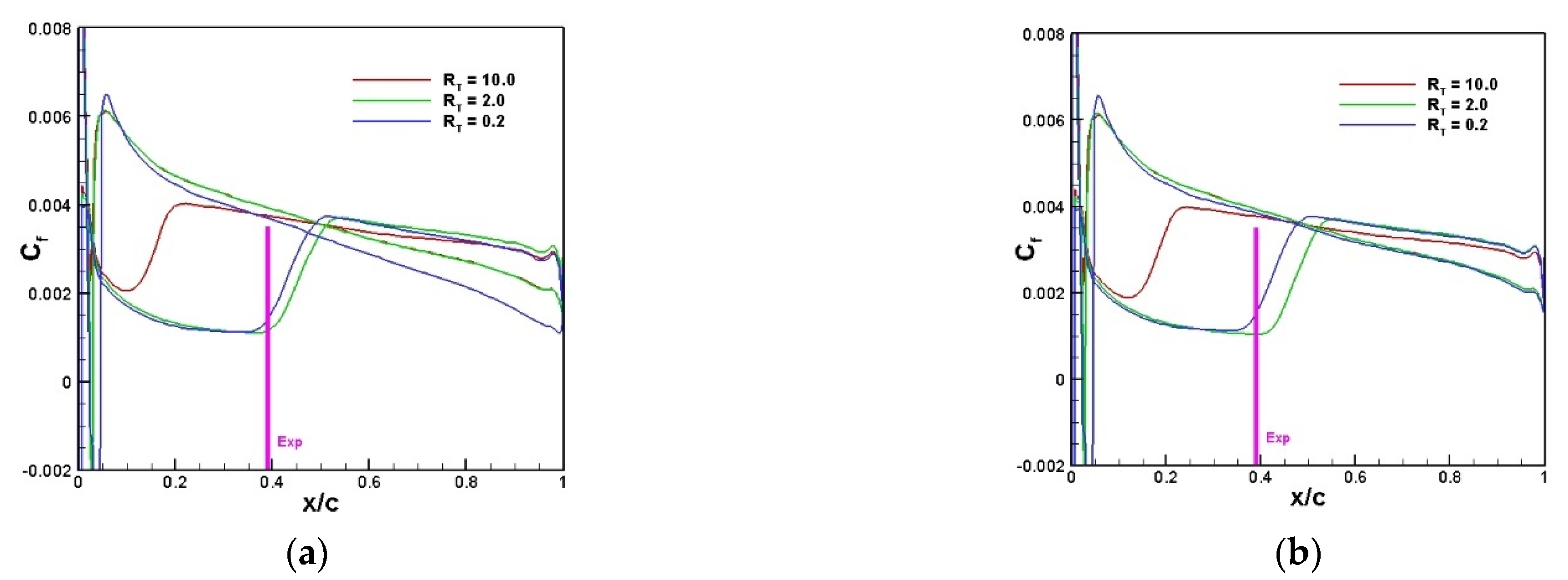
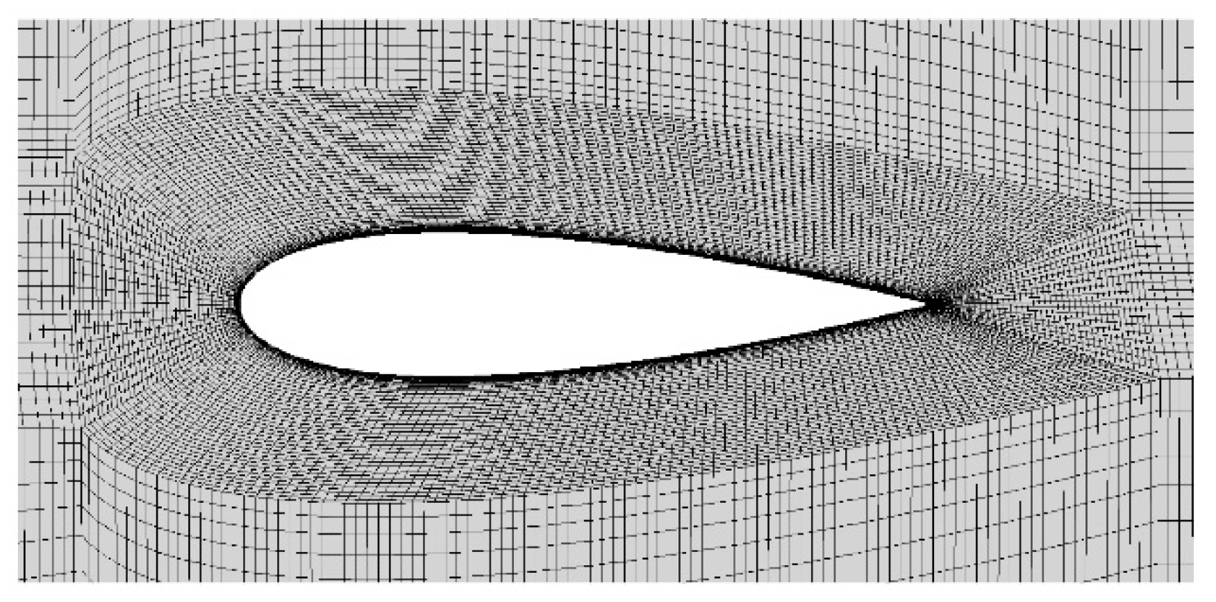
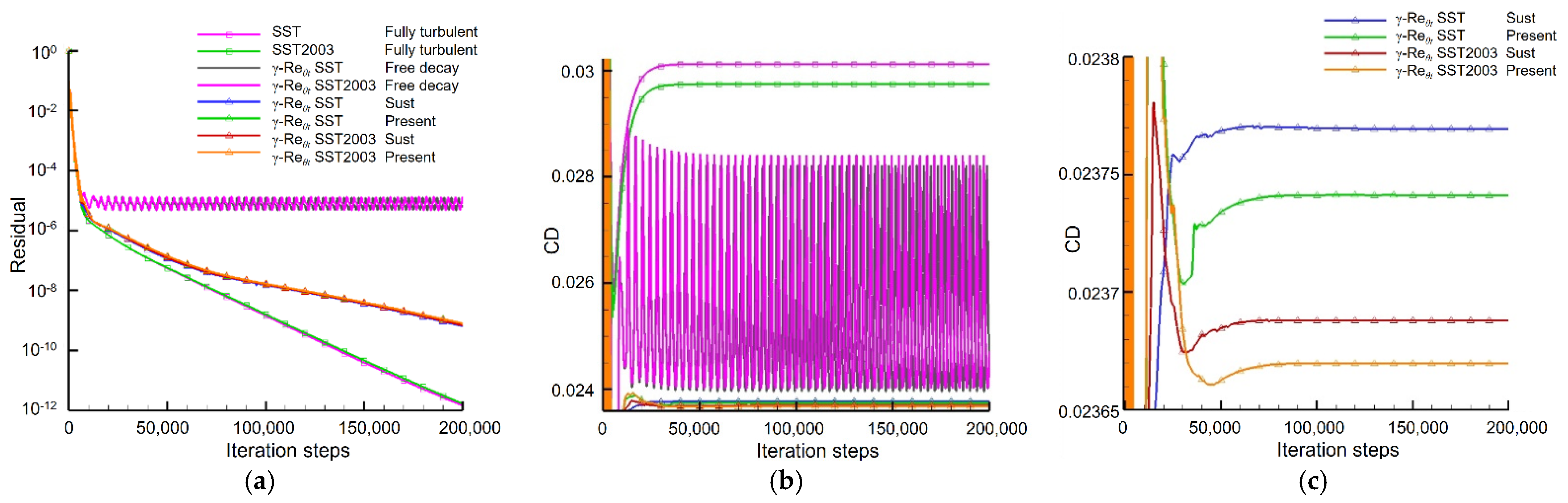
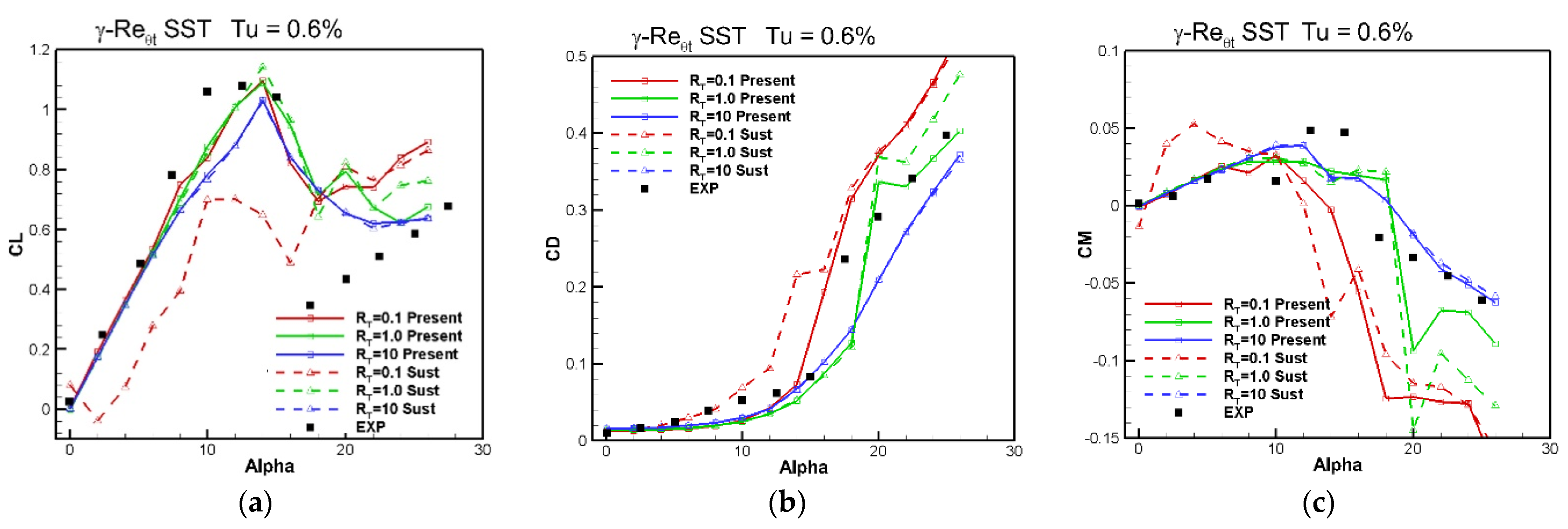
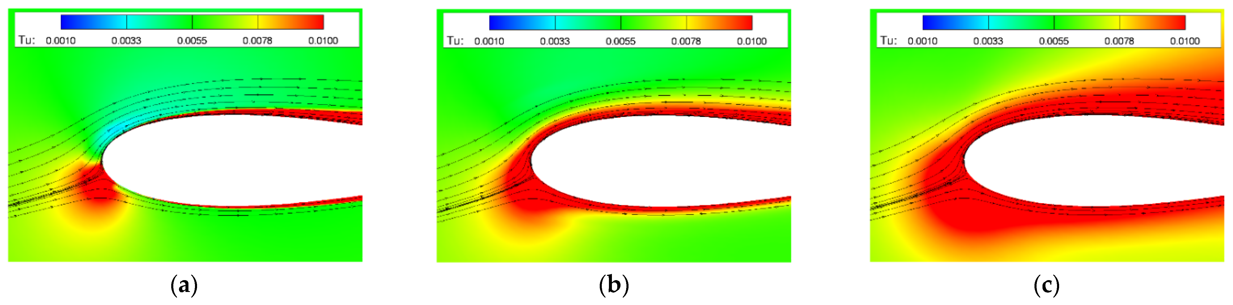
3.1. NACA0021 Airfoil

The NACA 0021 airfoil used here is experimental studied by Swalwel [30]. This airfoil can be used as horizontal axis wind turbine airfoil, so the flow condition is that the chord Reynolds number is Re = 2.7 × 10⁵ and the turbulence level quite high with Tu_FS = 0.6% in low-speed regime. This case is a challenging test case with transitional flow as well as flow separation on the trailing edge, and the abrupt stall occurs when laminar separation bubble merges with turbulent separation downstream, which was studied by Menter et al. [31] using their transition model to simulate the complex turbulent/transition behavior. For this computation, a very fine mesh is used with the grid expansion ratio in the boundary layer smaller than 1.1 used for such flows with small Reynolds numbers as depicted partly in Figure 1. The computation domain is very large; thus, the turbulence could decay to a very low value if no sustaining turbulence is used.

Figure 2 shows the convergence history for the standard SST, SST-2003, γ-Re_θt SST and γ-Re_θt SST-2003 with turbulence decay freely, the γ-Re_θt SST and γ-Re_θt SST-2003 models with the sustaining turbulence technology in [4] termed as ‘Sust’ and the proposed sustaining turbulence given in Equation (28) termed as ‘Present’. In order to obtain the same level freestream turbulence intensity in the vicinity to the airfoil, the sustaining turbulence technology is used with the inflow condition being set to FSTI = 0.6%, and R_T,FS is set to 2. The selected test case is at 10° of incidence, where the laminar separation bubble and the trailing edge separation appears together. The γ-Re_θt model with the free decaying of freestream turbulence cannot yield a steady solution. It is because the simulated large unsteady laminar separation bubble in the front of the airfoil makes the small trailing edge separation become unsteady as well; thus, the averaged residual cannot drop to a very low value. When the sustaining turbulence technology is used, the size of the laminar separation bubble becomes smaller and steady. The convergence history for the drag coefficient shows that, the convergence history of the force coefficient does not change after 50,000 iteration steps. In the following computations for NACA0021, all results are collected after 100,000 iteration steps.

All computations are run on the same computer with the same mesh, so there was no other CPU and memory cost when the computations were running. The final time consumptions after 200,000 iterations are listed in

Table 1. Time consumption for different turbulence/transition models (FD means free decay).

Turbulence/Transition Model	SST	SST2003	γ-Reθt SST FD	γ-Reθt SST-2003 FD	γ-Reθt SST Sust	γ-Reθt SST Present	γ-Reθt SST-2003 Sust	γ-Reθt SST-2003 Present
Time (s)	2188.6	2237.9	8600.5	7775.2	3746.9	3873.7	3620.9	3863.6
Time increment	1	1.02	3.93	3.55	1.71	1.77	1.65	1.77

. The computational time effort by standard SST model is used as a reference here. It is found that the SST-2003 model yields very close time consumption. The γ-Re_θt model has two more equations (Equations (3) and (4)) than the fully turbulent computation using SST-variants, and thus the time requirement is far larger. The γ-Re_θt model with sustaining turbulence saves a lot of time compared with the transition model with free decaying (FD). This is because the transition models with the free decay of turbulence yields large unsteady laminar separation bubble, which makes the additional inner iterations in the Re_θt-equation very difficult to converge. While for the sustaining turbulence proposed here, the time consumption is slightly higher than the sustaining turbulence technology in [4] due to Equation (28), which needs to perform three extra comparisons.

Figure 3 shows the turbulence intensity around the airfoil at the leading edge computed by SST-2003, γ-Re_θt SST, and γ-Re_θt SST-2003 at α = 8°, and the turbulence in the freestream decays freely; thus, the turbulent intensity in the vicinity of the airfoil is far lower than the 0.6% that was measured in the experiment. The computed force coefficients computed by SST-2003, γ-Re_θt SST, and γ-Re_θt SST2003 are depicted in Figure 4. The lift coefficient (CL) computed without considering flow transition is lower than the measurement when α < 10°, and the simulations using γ-Re_θt SST model and γ-Re_θt SST2003 model without controlling the turbulence decaying yield equally good accuracy. Small differences between the two variants of the transitional SST(-2003) model is observed due to Equation (8), which makes the SST-2003-based model yield a lower value of transport momentum thickness Reynolds number Re_θt. As a result, the turbulence intensity predicted by the γ-Re_θt SST model near the boundary layer of the airfoil is higher than the γ-Re_θt SST-2003 model near the leading edge. Due to the different level of turbulence intensity around the leading edge, the laminar separation bubble predicted by the γ-Re_θt SST model is smaller than by the γ-Re_θt SST-2003 model. Since the γ-Re_θt model is specifically designed to take the influence of freestream turbulence intensity into consideration, the transition location varies with the different levels of the freestream turbulence intensity, and the current case the transition model yields good accuracy with the wrong freestream turbulence intensity around the airfoil, which indicates that the current framework of the γ-Re_θt model needs improvements with respect to taking the ambient turbulence into consideration. For the force coefficients computed at α >18°, massive separation occurs; therefore, the current steady RANS computation cannot yield the correct solution and is not discussed further here.

The sustaining turbulence approach from [4] and the present approach coupled with the γ-Re_θt SST model are shown in Figure 5. The two sustaining turbulence terms yield significantly different behaviors as the turbulent viscosity ratio varies from 0.1 to 10. The present approach yields more robust results with different setting of R_T,FS, but the force coefficients are still sensitive to it. Figure 6 gives the behavior of the two sustaining turbulence terms coupled with the γ-Re_θt SST-2003 model, and the robustness of the sustaining terms is improved. The present approach yields almost identical force coefficients at small angles of attack. For higher angles of attack, the small value of the R_T,FS yields a poor solution with the present sustaining turbulence term, but it is better than the approach in [4], which adds too high a level of ω into the boundary layer and causes unphysical flow separation.

Figure 7 and Figure 8 depict the distribution of the turbulence intensity around the airfoil. Both SST-variants with the present sustaining turbulence term yield very close result with the same setting of R_T,FS. The freestream turbulence intensity is kept at 0.6%, not far from the airfoil. However, the turbulence intensity in the vicinity of the airfoil grows as R_T,FS increases. The stagnation point anomaly is significant, and the unphysical high turbulence at the nose of the airfoil becomes worse with higher R_T,FS, which is why the sensitivity to the initial freestream value of ω is introduced to the final result.

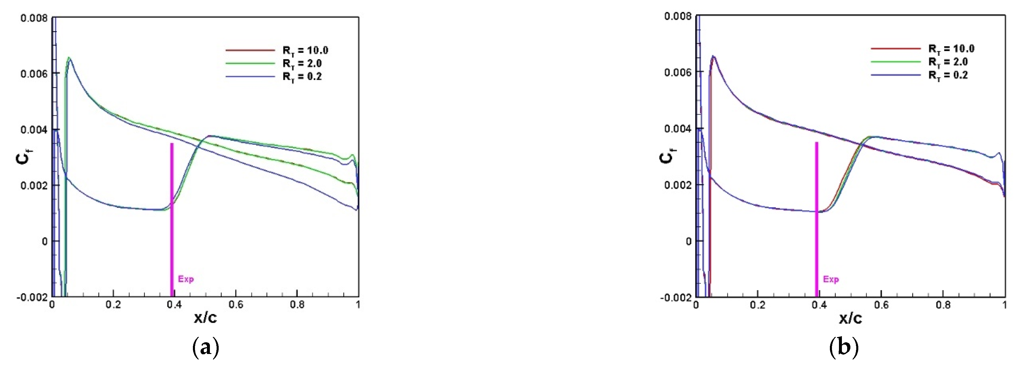
3.2. ONERA-D Infinite Swept Wing

The Onera-D infinite swept wing [32] is a typical crossflow-transition-dominated test for cases at certain swept angles and angles of attack. The freestream turbulence intensity of the ONERA S2 low-speed wind tunnel is around 0.2%. The selected case is Φ = 50° and Re_c = 1.0 × 10⁶, at which transition is onset due to crossflow instabilities on the pressure side at x_tr/c = 0.39. The γ-Re_θt-CF approach is used here with different settings of the turbulence viscosity ratio R_T at the far-field boundary. The transition location is not considered in this study because the transition model coupled with the sustaining turbulence technology requires recalibration. In the simulation, the computation domain is very large as well, and the mesh has an expansion ratio of 1.1, away from the surface of the wing. The main focus is to investigate the influence of the settings on the turbulent variants for the location of the crossflow transition.

The skin friction coefficients (C_f) on both pressure side and suction side are plotted together in Figure 9 and Figure 10, and the transition locations from the simulations are the middle point of the places where the surface skin reaches its minimum and maximum during transition processes, as illustrated in

Table 2. Transition locations verse different values of R_T,FS.

	RT,FS	0.2	2.0	10
Transition Models
γ-Reθt SST	Sust [4]	0.430	0.451	0.155
γ-Reθt SST-2003	Sust [4]	0.440	0.442	0.442
γ-Reθt SST	Present	0.425	0.468	0.185
γ-Reθt SST-2003	Present	0.486	0.485	0.481
Exp		0.39

. The leading-edge separation bubble can be identified clearly on the C_f -distributions, which is negative when the flow separates. For the γ-Re_θt-CF SST transition model as given in Figure 9, the transition location is very sensitive to the freestream value of R_T for two sustaining turbulence approaches. However, the skin friction coefficient computed with smaller R_T,FS for sustaining turbulence approach in [4] is smaller in the turbulence region near the trailing edge than that with higher R_T,FS, which is wrong. The reason behind this is still due to the high value of ω entering the boundary layer and causing unphysical trailing-edge low surface friction and even flow separation for even lower R_T,FS, as already shown in the NACA0021 case. The present sustaining turbulence approach yields almost coincident surface skin friction coefficient distribution in the rear part of the wing. For the γ-Re_θt-CF SST-2003 transition model, as given in Figure 10, almost identical results for R_T,FS = 2 and 10 but low skin friction coefficients at the rear of the airfoil occur again when R_T,FS = 0.2 for the sustaining turbulence approach in [4]. The present sustaining turbulence approach obtains almost the same skin friction coefficients for different values of R_T, which means the solution is likely to obtain the independent solution for the freestream value. Though the transition location moves downstream as R_T is increasing, the deviation is negligible.

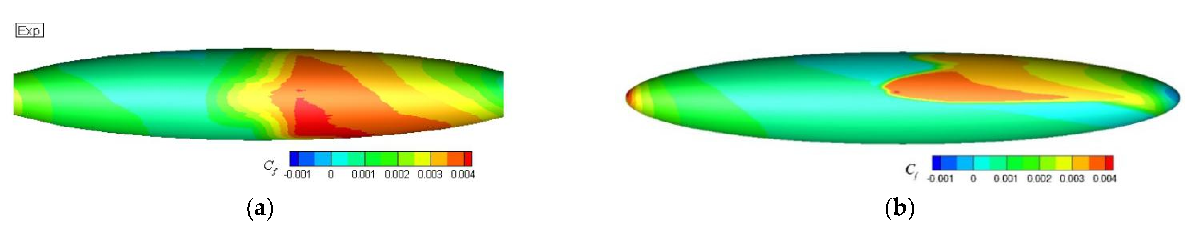
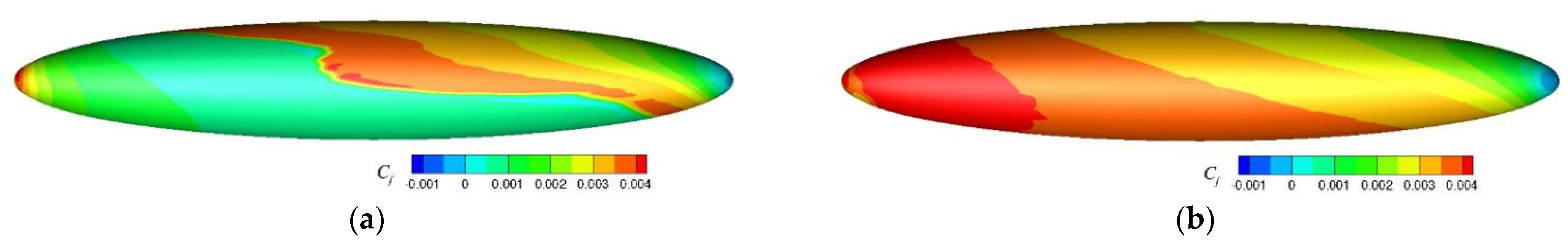
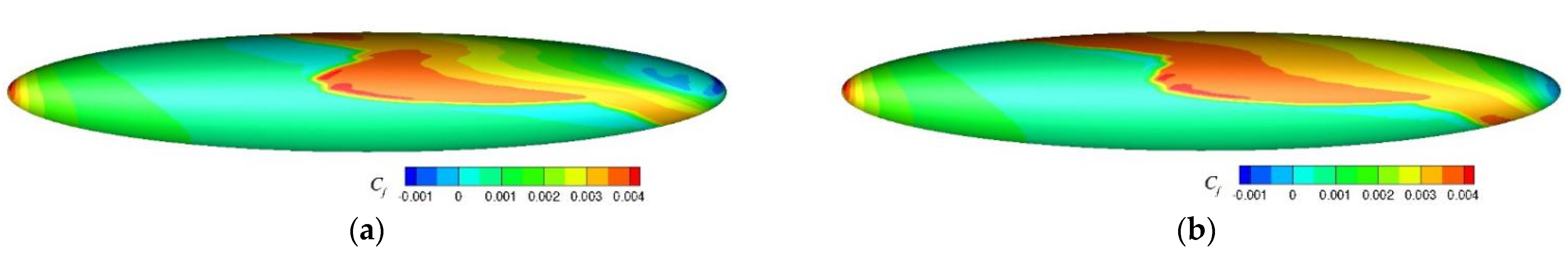
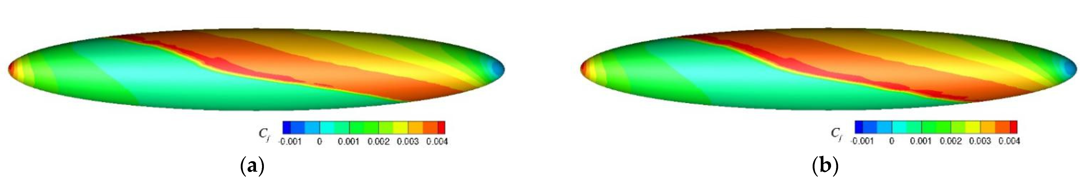
3.3. DLR 6:1 Prolate Spheroid

The 6:1 prolate-inclined spheroid is a very famous three-dimensional test case with different transition mechanisms at different Reynolds numbers. The local shear stresses were measured by hot film probes, which the turbulence model authors are very fond of. The selected test case has a Reynolds number of Re = 6.5 × 10⁶, and both T-S transition and CF transition occurs together at different angles of attack. A detailed study on this case can be found in [33]. In the simulation, the computation domain is very large and the mesh in the wall-normal direction has a grid expansion ratio of 1.05 to obtain a grid-independent solution. The freestream turbulence in the measurement is between 0.1–0.3%, and the stability analysis by Krimmelbein et al. [34] for the T-S instability is about 8, corresponding to a value of turbulence intensity of Tu = 0.106% according to Mack’s formulation (N_TS = −8.43–2.4 ln(Tu)), which yields very promising accuracy for is very fond by T-S transition on the windward and leeward of the spheroid. Here, only the case with α = 5° is investigated to demonstrate the influence of is very fond by sustaining turbulence term. At this angle of attack, the left half of the spheroid is turbulent. However, the transition model fails to predict the transition on the windward of the spheroid (lower surface). Here, the freestream turbulence is set to Tu = 0.35% to investigate the influence of the present sustaining turbulence technology only.

The results without sustaining turbulence term are given in Figure 11. The turbulence intensity in the vicinity of the spheroid decays freely to zero. The computed skin friction is comparable with other computations and can be found in [13,34]. Still, the flow is laminar on the windward surface, which is not comparable with the two-N-factor strategy [34] result or the measurement [33], but the transition line on the right top agrees well with the experimental data. As mentioned before, the transition model yields good transition locations with zero turbulence intensity around the spheroid, which is not the case in the wind tunnel.

The surface skin friction coefficient computed by the sustaining turbulence approach in [4] coupling with the standard SST model as plotted in Figure 12. The transition location is very sensitive to R_T,FS in comparison to the 2D cases. R_T,FS increases to five yields, an almost fully turbulent result, so this approach is not recommended for industrial application.

For the present sustaining turbulence approach coupled with the γ-Re_θt-CF SST-2003 model, the skin friction coefficient varying with R_T,FS from 0.1 to 10 are depicted in Figure 13 and Figure 14. The present sustaining technology coupled with the standard SST yield the similar distribution of surface friction, and the drag coefficient computed by different approach are given in

Table 3. Drag coefficients for different approaches.

	RT,FS	0.1	1.0	5.0	10.0
Transition Models
γ-Reθt SST-2003	free decay	0.0046	Not computed
γ-Reθt SST	Present	0.0071	0.0056	0.0065	0.0065
γ-Reθt SST-2003	Present	0.0069	0.0057	0.0064	0.0064

. The transition location still varies with different values of R_T,FS, but the difference in between is far smaller in comparison to the computation given in Figure 12. When R_T,FS increases from 0.1 to 1, the crossflow transition in the middle of the spheroid does not change, but the T-S transition on the upper part of the spheroid moves downstream. Still, when R_T,FS = 0.1, the skin friction coefficient on the rear of the spheroid is too low, as already found for the 2D cases, which may be unphysical and cause higher drag. When the value of R_T,FS increases from 1 to 10, the skin friction moves upstream on the upper and lower surfaces as well as in the middle of the surface. The results predicted by setting R_T,FS = 5 and 10 are almost identical, thus the drag. However, the transition on the lower surface cannot move to further upstream as observed in the experiments, which implies that the current framework of the γ-Re_θt-CF model is not able to predict the T-S transition on the windward side of the spheroid, even with the turbulence intensity being 0.35% around the geometry. The error cannot be fixed by changing the turbulence intensity at the far-field or the coupled SST model version, thus a possible source of error due to the empirical transition criterion in the γ-Re_θt-CF model fails in the weak favorable pressure gradient (FPG) region.

4. Conclusions

For transition prediction using a transport-equation-based approach, the prediction of the transition location is very interesting to the CFD community, but the simulation results are also usually questioned by engineers. The transition location could be different due to mesh qualities, turbulence initializations, and model calibration. For flow physics, the simulation should produce the same freestream turbulence intensity at first. In order to yield the same turbulence level in large computational domains for transition prediction, the sustaining turbulence technology can be used to maintain the suitable turbulence intensity. Two SST variants, the standard SST model and the SST-2003 model, were investigated coupling with the sustaining turbulence approach shown here, but the modeling of sustaining turbulence terms and adding to the transport equation introduces the sensitivity of the initial value of ω to the result again. A new approach to control the turbulence decay in the freestream without adding an ambient production contribution into the boundary layer is proposed and validated with three test cases, and the sensitivity of the transition prediction using different approaches to the initial turbulence value of ω and R_T,FS is compared and shown. The conclusions can be drawn as the following:

1. The SST-2003 model is more suitable than standard SST model regarding the transition behavior for attached flow. The good prediction is due to the limiter in Equation (8), which prevents the production of the k-equation from exceeding 10 times the destruction. Thus, this model variant yields lower levels of turbulence near the leading edge of the airfoil.

2. The present proposed sustaining turbulence approach, without adding the contribution of additional sustaining turbulence term to the boundary layer in conjunction with the SST-2003, reduces sensitivity to the freestream value for low R_T,FS.

3. The modified sustaining turbulence approach in conjunction with the standard SST model still has great dependence to the freestream turbulence value ω, and this cannot be prevented because the turbulent viscosity ratio is used in the transition model as switch functions such as F_onset3 and F_turb. The sensitivity becomes greater for three-dimensional flow.

4. For the use of the transition model with sustaining turbulence, the SST-2003 model as well as the R_T,FS in the ambient term being set to a value higher than 1 are highly recommended. This could yield physical solution and make the comparison between different CFD users more reasonable.

5. For other transport-equation-based transition models, since the turbulent viscosity ratio is always used in the onset function or switch functions, the conclusions drawn in this paper fit for other local-based transport transition models.

6. The proposed approach is only tested for attached flow, and it is not tested for flow with laminar to turbulent transition and massive separation together, on which the sensitivity of the model to the freestream value of R_T,FS is not clear. The λ₂-criteria [35] and the vortex structure will be presented in the future.

References

1. Langtry, R.B.; Menter, F.R. Correlation-based transition modeling for unstructured parallelized computational fluid dynamics codes. AIAA J. 2009, 47, 2894–2906. [Google Scholar] [CrossRef]
2. Suluksna, K.; Juntasaro, E. Assessment of intermitte ncy transport equations for modeling transition in boundary layers subjected to freestream turbulence. Int. J. Heat Fluid Flow 2007, 29, 48–61. [Google Scholar] [CrossRef]
3. Rumsey, C.L.; Lee-Rausch, E.M. NASA trapezoidal wing computations including transition and advanced turbulence modeling. J. Aircr. 2014, 52, 496–509. [Google Scholar] [CrossRef]
4. Seyfert, C.; Krumbein, A. Evaluation of a correlation-based transition model and comparison with the eN method. J. Aircr. 2012, 49, 1765–1773. [Google Scholar] [CrossRef]
5. Halila, G.L.O.; Antunes, A.P.; Silva, R.G.; Azevedo, J.L.F. Effects of boundary layer transition on the aerodynamic analysis of high-lift systems. Aerosp. Sci. Technol. 2019, 90, 233–245. [Google Scholar] [CrossRef]
6. Grabe, C.; Krumbein, A. Extension of the γ-Reθt model for prediction of crossflow transition. In Proceedings of the 52nd Aerospace Science Meeting, AIAA Paper 2014-1269. National Harbor, MD, USA, 13–17 January 2014. [Google Scholar]
7. Choi, J.H.; Kwon, O.J. Enhancement of a correlation-based transition turbulence model for simulating crossflow instability. AIAA J. 2015, 53, 3063–3072. [Google Scholar] [CrossRef]
8. Xu, J.K.; Bai, J.Q.; Qiao, L.; Zhang, Y. Correlation-based transition transport modeling for simulating crossflow instabilities. J. Appl. Fluid Mech. 2016, 9, 2435–2442. [Google Scholar] [CrossRef]
9. Arnal, D.; Habiballah, M.; Coustols, E. Laminar instability theory and transition criteria in two and three-dimensional flow. Rech. Aerosp. 1984, 2, 45–63. [Google Scholar]
10. Müller, C.; Herbst, F. Modeling of crossflow induced transition based on local variables. In Proceedings of the 6th European Conference on Computational Fluid Dynamics (ECFD VI), Barcelona, Spain, 20–25 July 2014. [Google Scholar]
11. Langtry, R.B.; Sengupta, K.; Yeh, D.T.; Dorgan, A.J. Extending the γ-Reθt local correlation based transition model for crossflow effects. In Proceedings of the 45th AIAA Fluid Dynamics Conference, Dallas, TX, USA, 22–26 June 2015. AIAA paper 2015–2474. [Google Scholar]
12. Medida, S.; Baeder, J. A new crossflow transition onset criterion for RANS turbulence models. In Proceedings of the 21st AIAA Computational Fluid Dynamics Conference, AIAA paper 2013–3081. San Diego, CA, USA, 24–27 June 2013. [Google Scholar]
13. Grabe, C.; Nie, S.Y.; Krumbein, A. Transport modeling for the prediction of crossflow transition. AIAA J. 2018, 56, 3167–3178. [Google Scholar] [CrossRef]
14. Langtry, R. A Correlation-Based Transition Model Using Local Variables for Unstructured Parallelized CFD Codes. Ph.D. Thesis, Univ. of Stuttgart, Stuttgart, Germany, 2006. [Google Scholar]
15. Savill, A.M. Some Recent Progress in the Turbulence Modelling of By-Pass Transition, Near-Wall Turbulent Flows; So, R.M.C., Speziale, C.G., Launder, B.E., Eds.; Elsevier: New York, NY, USA, 1993; p. 829. [Google Scholar]
16. Bode, C.; Aufderheide, T.; Friedrichs, J.; Kožulović, D. Improved Turbulence and Transition Prediction for Turbomachinery Flows. In Proceedings of the ASME 2014 International Mechanical Engineering Congress and Exposition, Montreal, QC, Canada, 14–20 November 2014. [Google Scholar]
17. Spalart, P.; Rumsey, C. Effective inflow conditions for turbulence models in aero-dynamic flows. AIAA J. 2007, 45, 2544–2553. [Google Scholar] [CrossRef]
18. Turbulence Modeling Resource. Available online: http://turbmodels.larc.nasa.gov (accessed on 5 July 2022).
19. Menter, F.R. Two-equation eddy-viscosity turbulence models for engineering applications. AIAA J. 1994, 32, 1598–1605. [Google Scholar] [CrossRef] [Green Version]
20. Menter, F.R. Improved Two-Equation k-Omega Turbulence Models for Aerodynamic Flows. NASA-TM-103975, October 1992. Available online: https://ntrs.nasa.gov/citations/19930013620 (accessed on 3 March 2022).
21. Menter, F.R.; Kuntz, M.; Langtry, R. Ten years of industrial experience with the SST turbulence model. In Turbulence, Heat and Mass Transfer, 4th ed.; Hanjalic, K., Nagano, Y., Tummers, M., Eds.; Begell House, Inc.: Danbury, CT, USA, 2003; pp. 625–632. [Google Scholar]
22. Sorensen, N. Prediction of airfoil performance at high Reynolds numbers. In Proceedings of the EFMC 2014, Copenhagen, Denmark, 17–20 September 2014. [Google Scholar]
23. Diakakis, K.; Papadakis, G.; Voutsinas, S.G. Assessment of transition modeling for high Reynolds flows. Aerosp. Sci. Technol. 2019, 85, 416–428. [Google Scholar] [CrossRef]
24. Ströer, P.; Krimmelbein, N.; Krumbein, A.; Grabe, C. Stability-based transition transport modeling for unstructured computational fluid dynamics including convection effects. AIAA J. 2020, 58, 1506–1517. [Google Scholar] [CrossRef]
25. Nie, S.Y.; Krimmelbein, N.; Krumbein, A.; Grabe, C. Coupling of a Reynolds stress model with the γ-Reθt transition model. AIAA J. 2018, 56, 146–157. [Google Scholar] [CrossRef]
26. Nie, S.Y.; Krimmelbein, N.; Krumbein, A.; Grabe, C. Extension of a Reynolds-stress-based transition transport model for crossflow transition. J. Aircr. 2018, 55, 1641–1654. [Google Scholar] [CrossRef]
27. Endo, S.; Sujisakulvong, T.; Kuya, Y.; Ariki, T.; Sawada, K. Laminar-turbulent transition modeling with a Reynolds stress model for anisotropic flow characteristics. In Proceedings of the AIAA Scitech 2020 Forum, AIAA paper 2020-1311. Orlando, FL, USA, 6–10 January 2020. [Google Scholar]
28. Zhou, L.; Gao, Z.H.; Du, Y.M. Flow-dependent DDES/γ-Reθt coupling model for the simulation of separated transitional flow. Aerosp. Sci. Technol. 2019, 87, 389–403. [Google Scholar] [CrossRef]
29. Nie, S.Y.; Wang, Y.; Liu, Z.Q.; Jin, P.; Jiao, J. Numerical investigation and discussion on CHN-TI benchmark model using Spalart-Allmaras model and SSG/LRR-ω model. Acta Aerodyn. Sin. 2019, 37, 310–319. (In Chinese) [Google Scholar]
30. Swalwel, K.E. The Effect of Turbulence on Stall of Horizontal Axis Wind Turbines. Ph.D. Thesis, Monash University, Victoria, Australia, 2005. [Google Scholar]
31. Menter, F.R.; Smirnov, P.E.; Liu, T.; Avancha, R. A one-equation local correlation-based transition model. Flow Turbul. Combust. 2015, 95, 583–619. [Google Scholar] [CrossRef]
32. Schmitt, V.; Manie, F. Écoulement subsoniques et transsoniques sur une aile a flèche variable. Rech. Aérospatiale 1979, 4, 219–237. [Google Scholar]
33. Kreplin, H.-P.; Vollmers, H.; Meier, H.U. Wall shear stress measurements on an inclined prolate spheroid in the DFVLR 3 m × 3 m low speed wind tunnel. Data Rep. DFVLR IB 1985, 222–284. [Google Scholar]
34. Krimmelbein, N.; Krumbein, A.; Grabe, C. Validation of transition modeling techniques for a simplified fuselage configuration. In Proceedings of the 2018 AIAA Aerospace Sciences Meeting, AIAA paper 2018-0030. Kissimmee, FL, USA, 8–12 January 2018. [Google Scholar]
35. Jeong, J.; Hussain, F. On the identification of a vortex. J. Fluid Mech. 1995, 285, 69–94. [Google Scholar] [CrossRef]
Figure 1. Mesh for NACA0021 (236 points on the surface of the airfoil and 143 points in wall-normal direction).
Energies 15 06491 g001
Figure 2. The convergence history for different turbulence/transition models. (a) Convergence history. (b) Drag coefficient vs. iteration steps. (c) Drag coefficient for different models.
Energies 15 06491 g002
Figure 3. Computed turbulence intensity distribution and streamlines at α = 8°. (a) SST-2003. (b) γ-Reθt SST. (c) γ-Reθt SST-2003. (“S” denotes separation point and “R” denotes reattachment point.)
Energies 15 06491 g003
Figure 4. Computed force coefficients predicted by different approaches versus experimental data. (a) Lift coefficient vs. AoA. (b) D rag coefficient vs. AoA. (c) Pitching moment coefficient vs. AoA.
Energies 15 06491 g004
Figure 5. Computed force coefficients predicted with sustaining term from [4] and present approach using γ-Reθt SST model. (a) Lift coefficient vs. AoA. (b) Drag coefficient vs. AoA. (c) Pitching moment coefficient vs. AoA.
Energies 15 06491 g005
Figure 6. Computed force coefficients predicted with sustaining term from [4] and present approach using γ-Reθt SST 2003 model. (a) Lift coefficient vs. AoA. (b) Drag coefficient vs. AoA. (c) Pitching moment coefficient vs. AoA.
Energies 15 06491 g006
Figure 7. Computed turbulence intensity distribution and streamlines predicted by γ-Reθt SST at α = 8°. (a) RT,FS = 0.1. (b) RT,FS = 1.0. (c) RT,FS = 10. (“S” denotes separation point and “R” denotes reattachment point.)
Energies 15 06491 g007
Figure 8. Computed turbulence intensity distribution and streamlines predicted by γ-Reθt SST-2003 at α = 8°. (a) RT,FS = 0.1. (b) RT,FS = 1.0. (c) RT,FS = 10.
Energies 15 06491 g008
Figure 9. γ-Reθt-CF SST transition model with different sustaining turbulence terms. (a) Sustaining turbulence approach in [4]. (b) Present approach.
Energies 15 06491 g009
Figure 10. γ-Reθt-CF SST2003 transition model with different sustaining turbulence terms. (a) Sustaining turbulence approach in [4]. (b) Present approach.
Energies 15 06491 g010
Figure 11. Experimental measurement (left) and computation using γ-Reθt-CF SST-2003. (a) Exp. (b) RT,FS = 0.1.
Energies 15 06491 g011
Figure 12. γ-Reθt-CF SST transition model with sustaining turbulence term in [4]. (a) RT,FS = 1.0. (b) RT,FS = 5.0.
Energies 15 06491 g012
Figure 13. γ-Reθt-CF SST-2003 transition model with present sustaining turbulence. (a) RT,FS = 0.1. (b) RT,FS = 1.0.
Energies 15 06491 g013
Figure 14. γ-Reθt-CF SST-2003 transition model with present sustaining turbulence. (a) RT,FS = 5.0. (b) RT,FS = 10.0.
Energies 15 06491 g014