
Energy Consumption Prediction and Analysis for Electric Vehicles: A Hybrid Approach

 , ,
, ,  , and
, and
Abstract
:1. Introduction
2. Vehicle Modeling
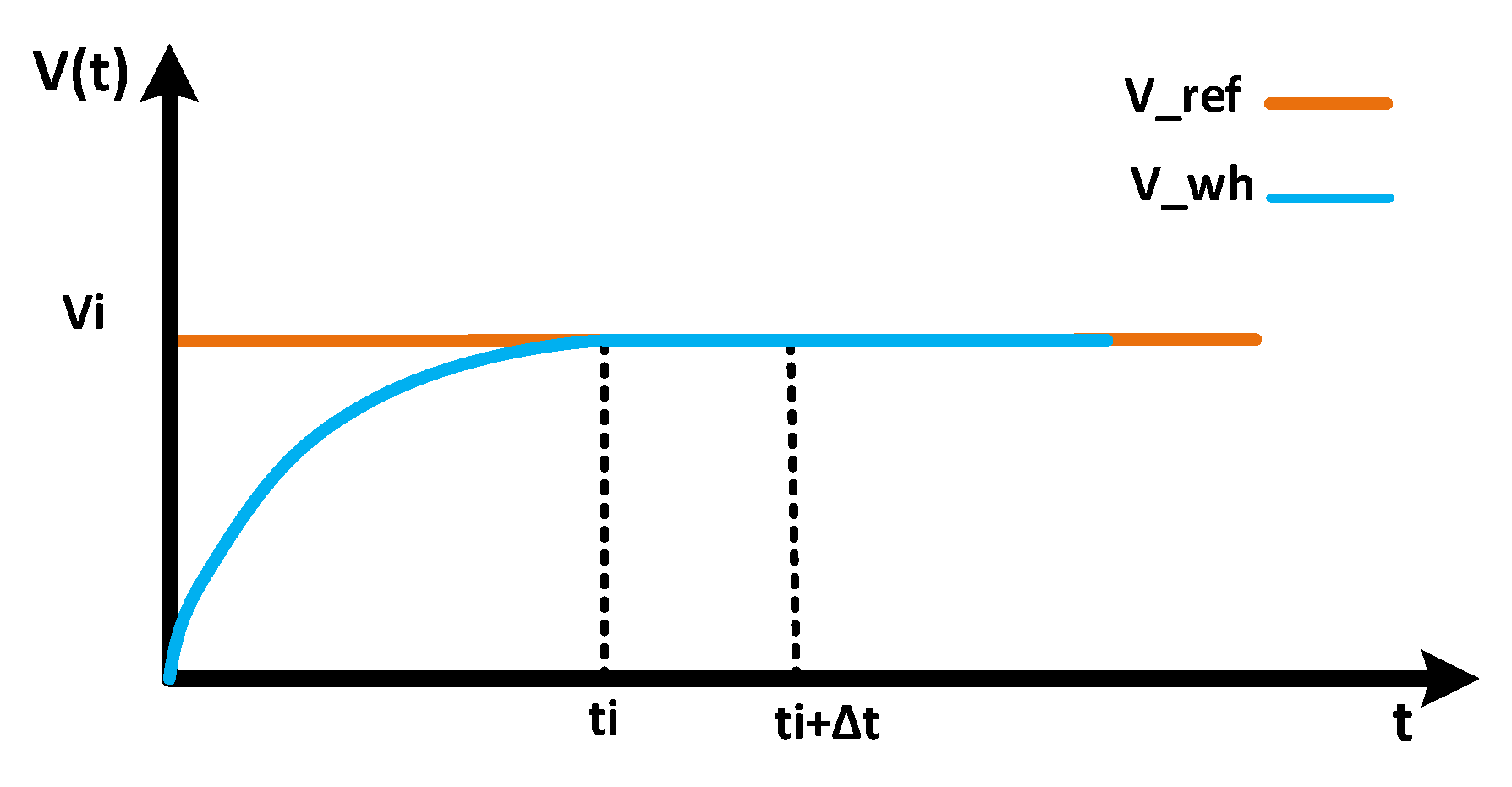
2.1. Driver Model
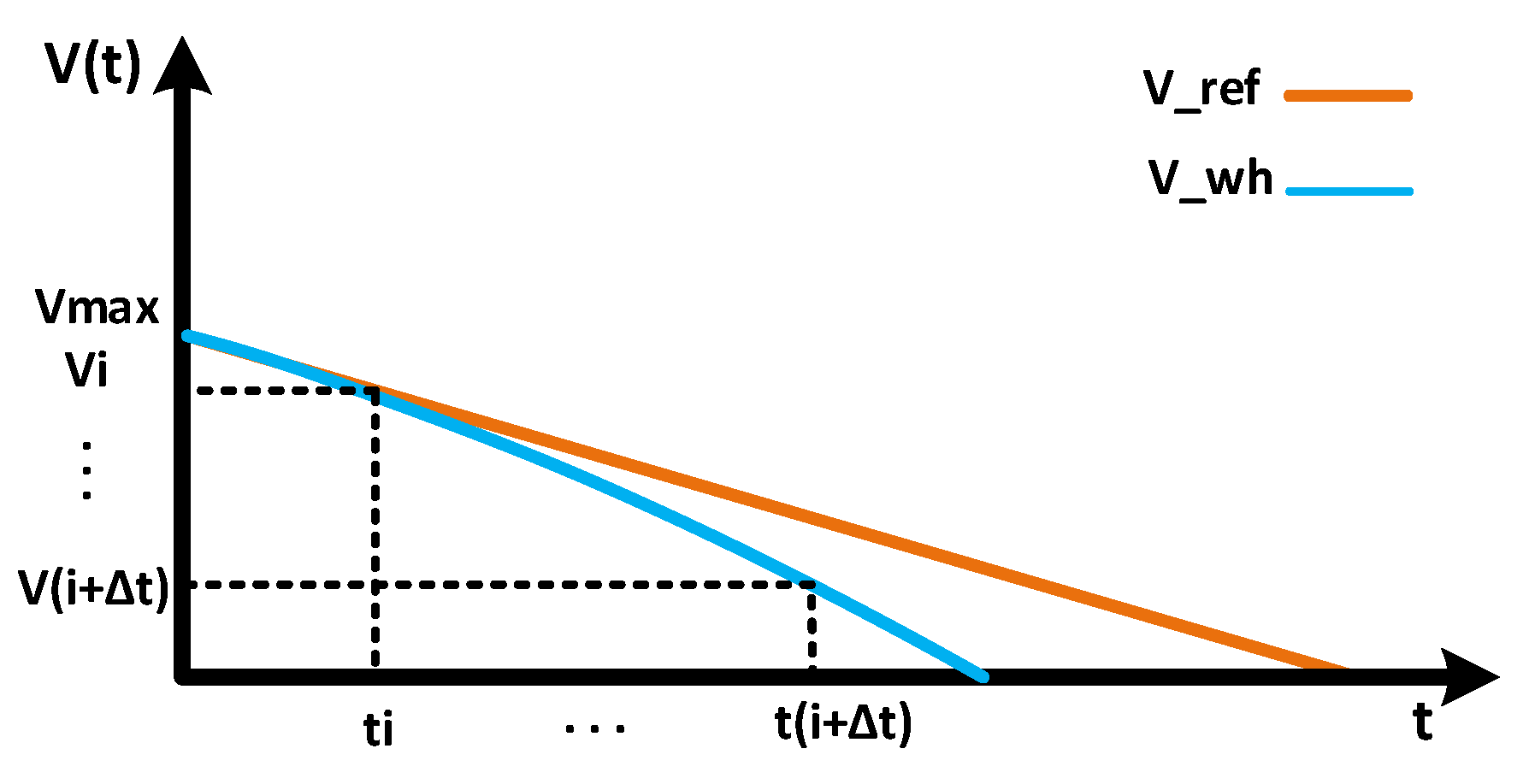
2.2. Braking Strategy Model
2.3. Electric Motor and Drive Electronics Model
2.4. Battery Model
2.5. Driveline and Transmission Model
2.6. Auxiliary Devices Model
2.7. Longitudinal Vehicle Dynamics
3. Standard Driving Cycles and Factors Impacting Energy Consumption
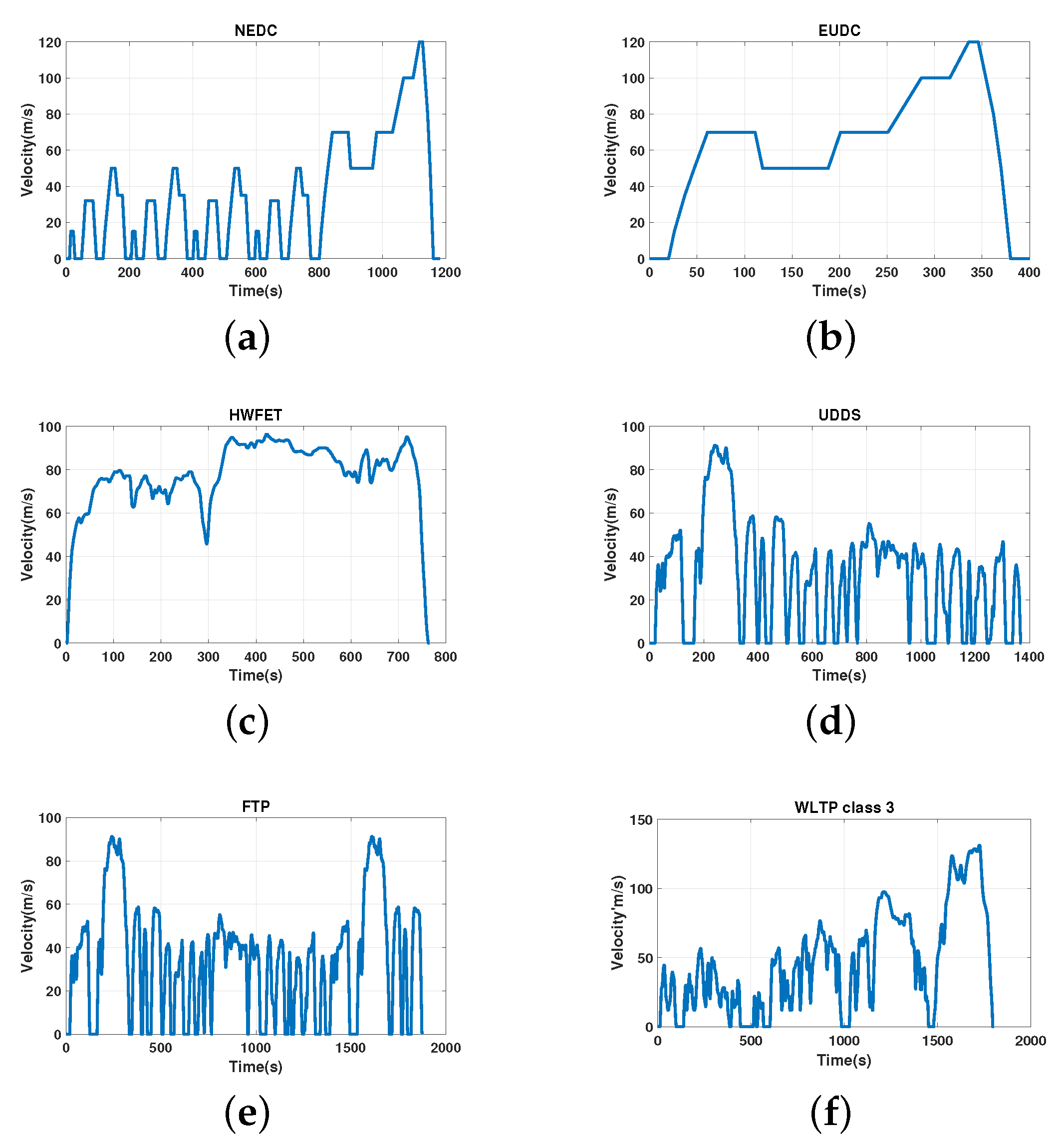
3.1. Standard Driving Cycles
3.2. Factors Impacting Energy Consumption
3.2.1. Vehicle Technology Factors
3.2.2. Driver Behavior
3.2.3. Climatic Conditions
3.2.4. Road Topography
3.2.5. Road Conditions
4. Synthetic Dataset Construction Methodology
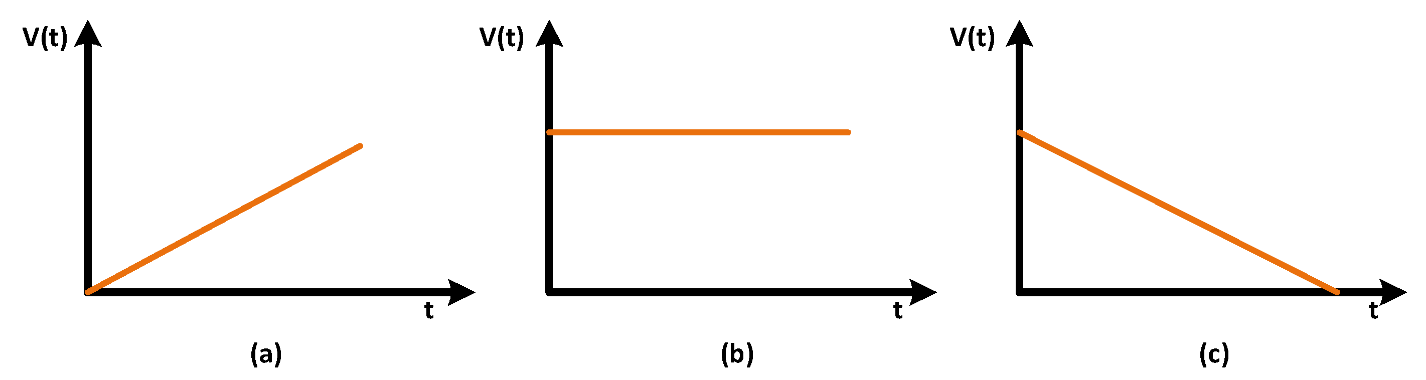
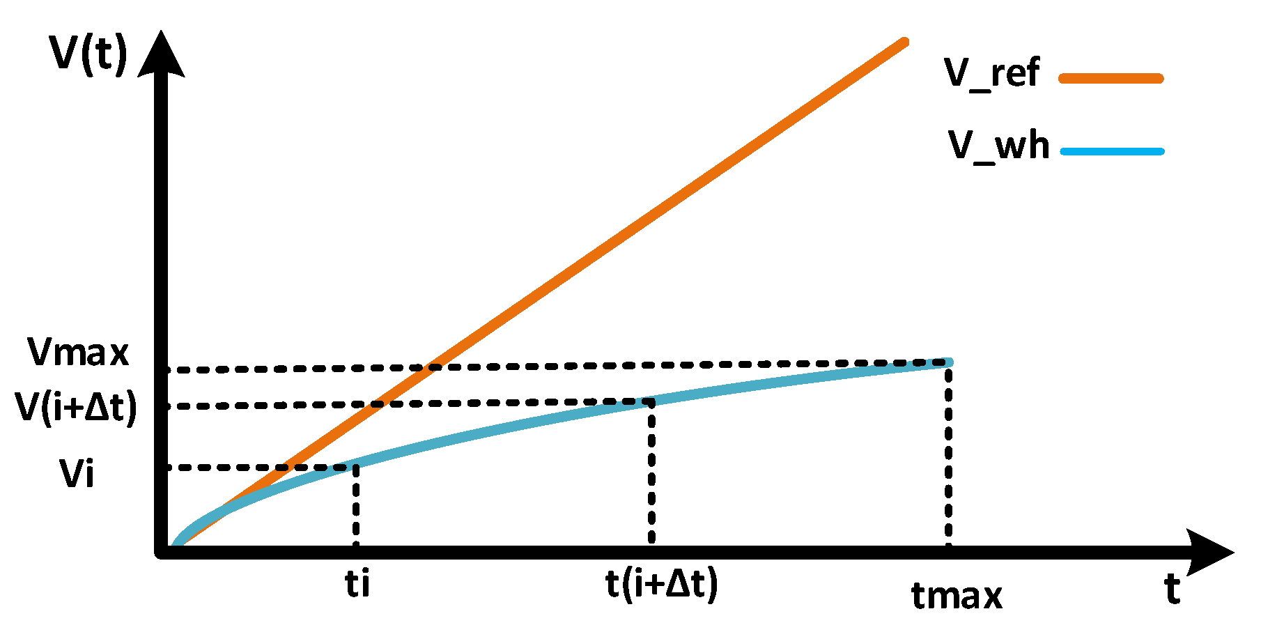
4.1. Synthetic Speed Profile Construction
4.2. Synthetic Dataset Construction
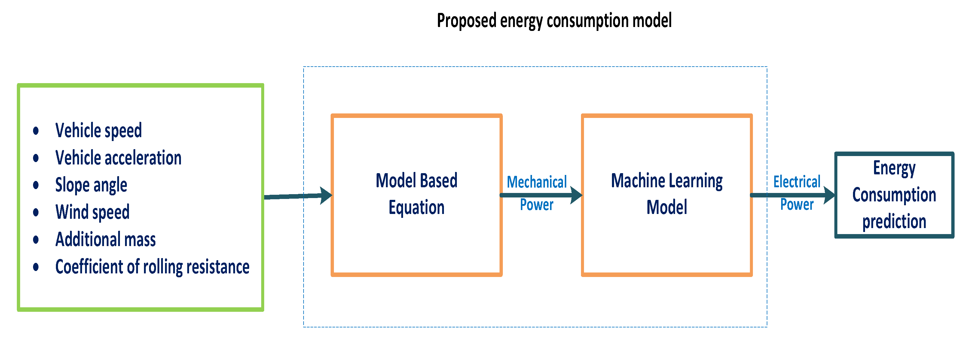
5. Proposed Energy Consumption Model
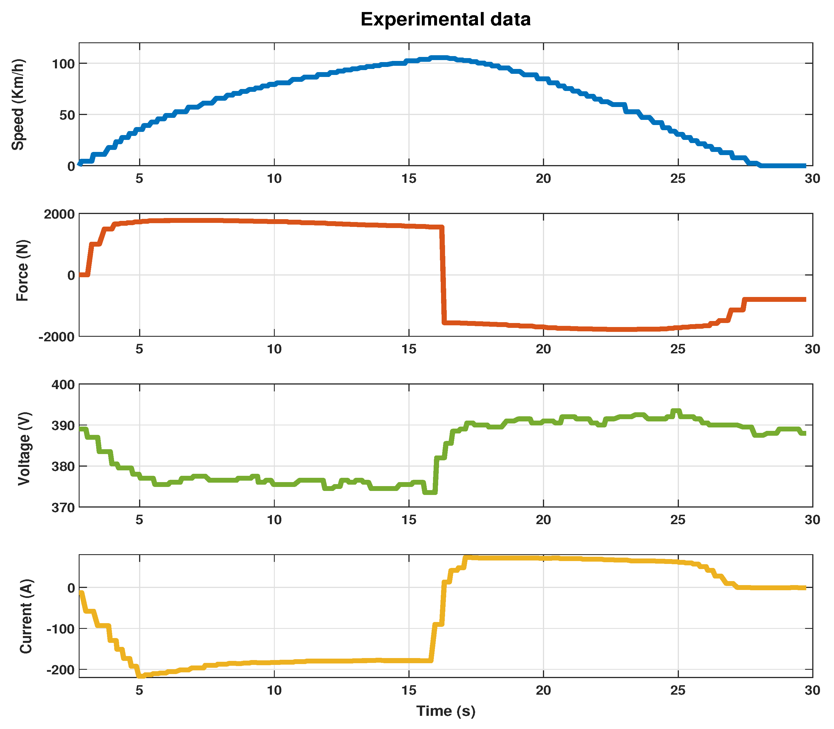
5.1. Real-World Measurement
5.2. Machine Learning Models
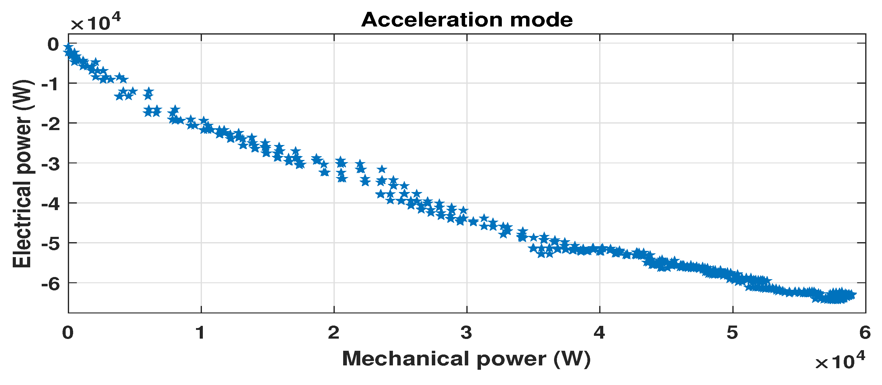
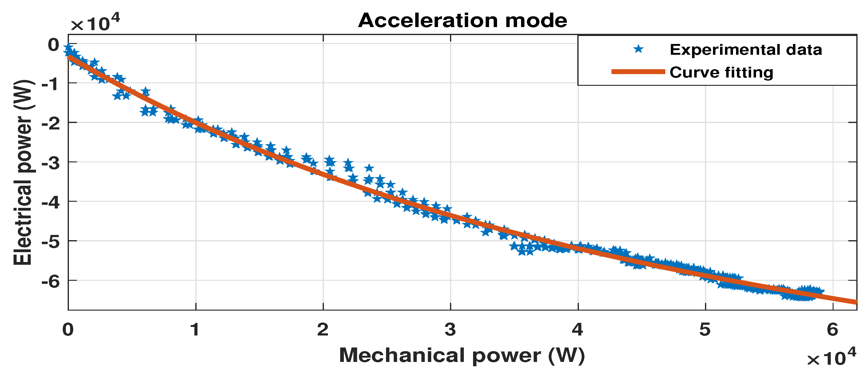
5.2.1. Acceleration Mode
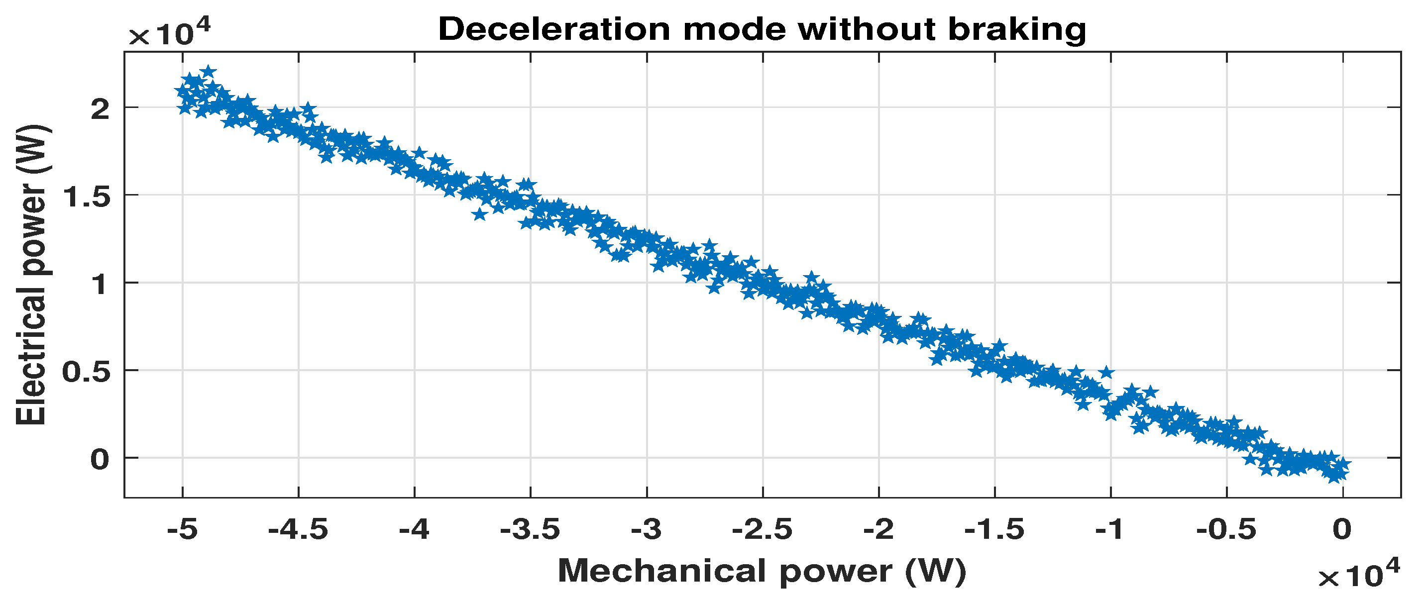
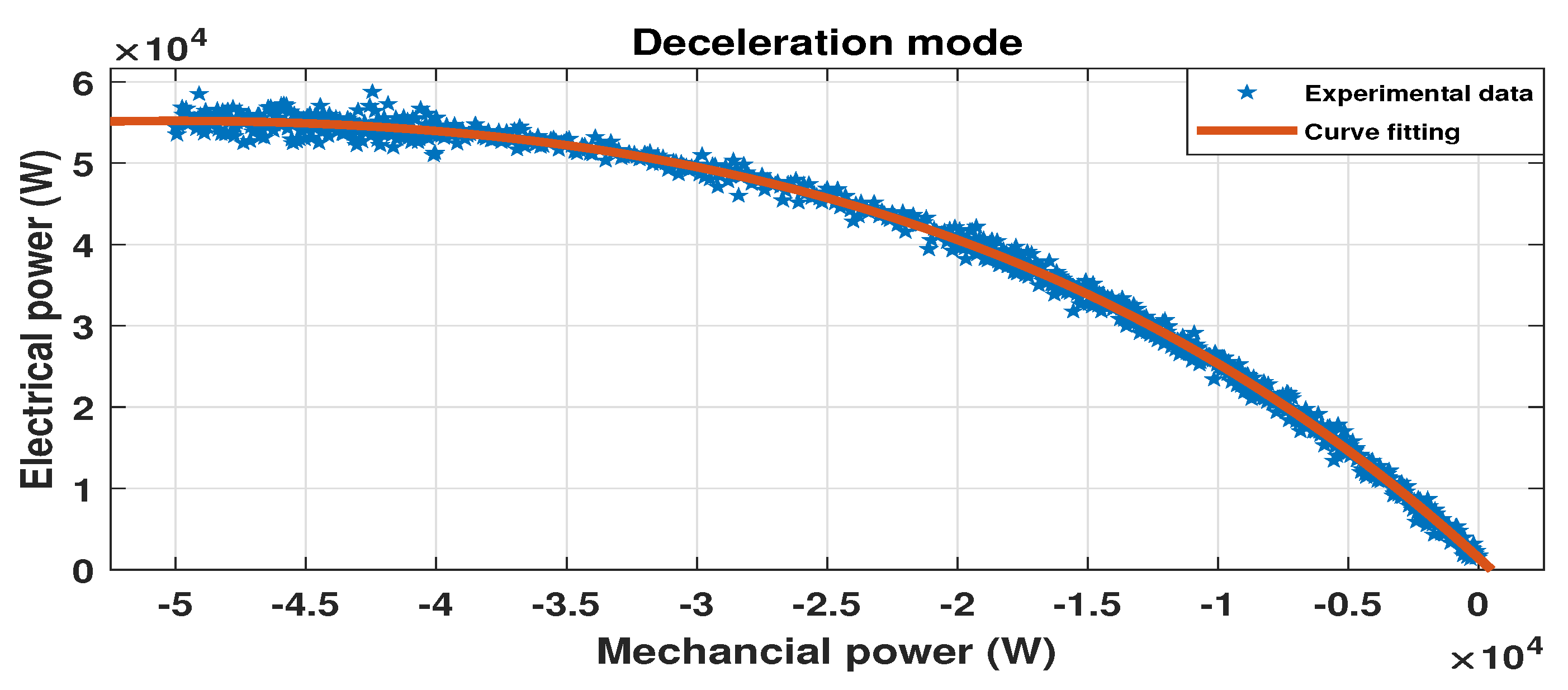
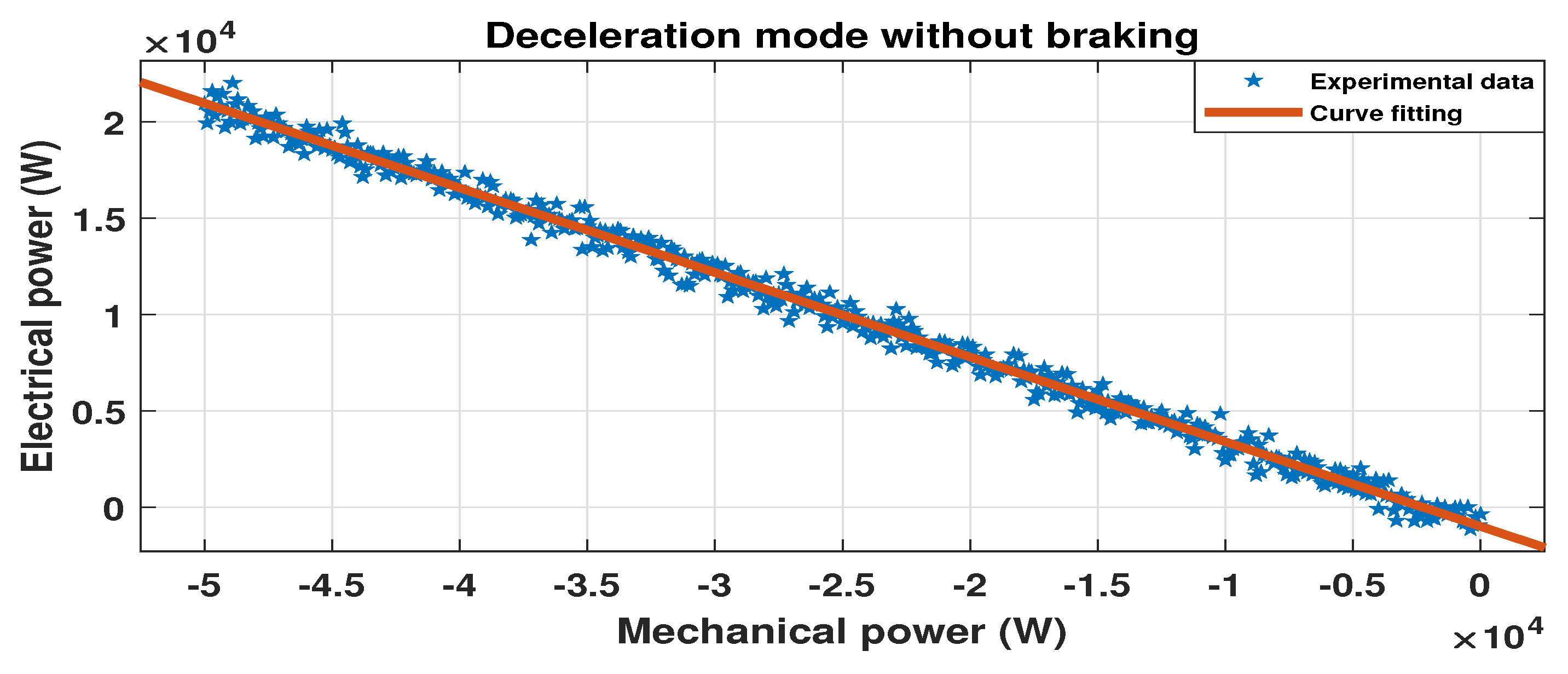
5.2.2. Deceleration Mode
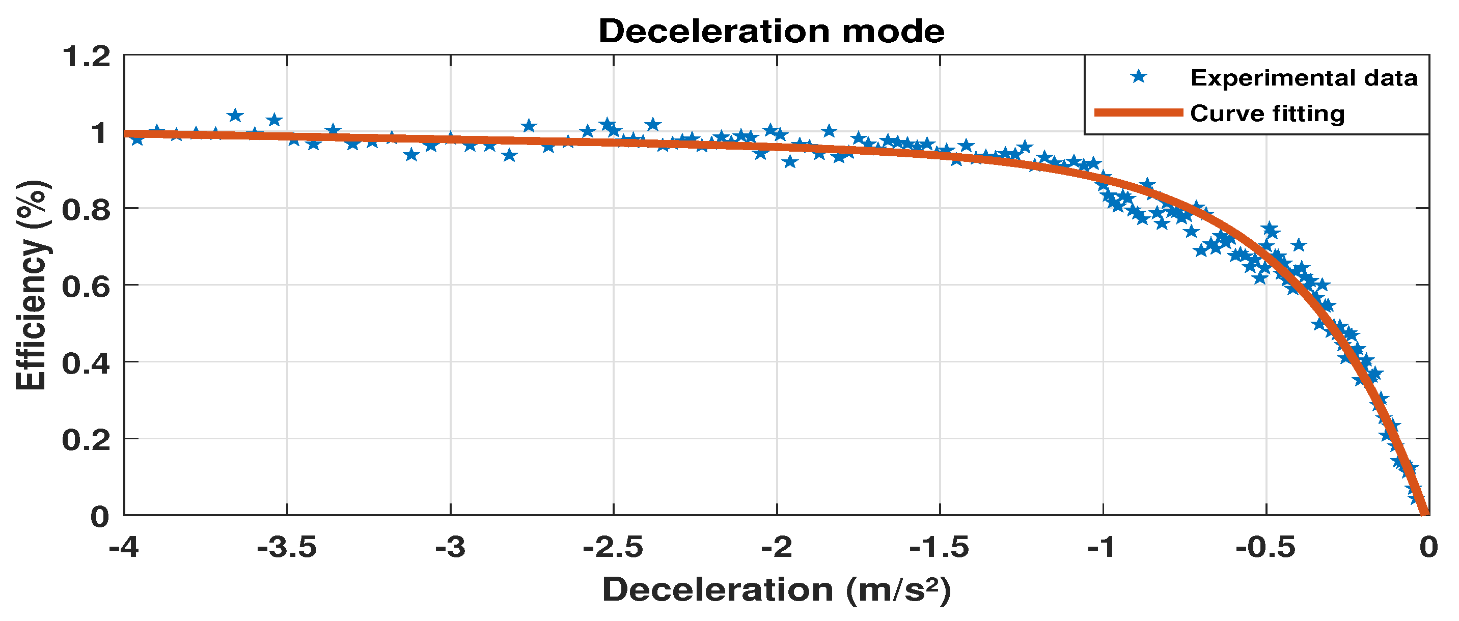
5.3. Regenerative Braking Power Efficiency as a Function of Deceleration
5.4. Results and Discussion
6. Conclusions
Author Contributions
Funding
Conflicts of Interest
References
- Genikomsakis, K.N.; Mitrentsis, G. A computationally efficient simulation model for estimating energy consumption of electric vehicles in the context of route planning applications. Transp. Res. Part D Transp. Environ. 2017, 50, 98–118. [Google Scholar] [CrossRef]
- Shankar, R.; Marco, J. Method for estimating the energy consumption of electric vehicles and plug-in hybrid electric vehicles under real-world driving conditions. IET Intell. Transp. Syst. 2013, 7, 138–150. [Google Scholar] [CrossRef]
- Salvucci, R.; Tattini, J. Global outlook for the transport sector in energy scenarios. In DTU International Energy Report 2019: Transforming Urban Mobility; DTU: Denmark, 2019; pp. 21–27. [Google Scholar]
- De Cauwer, C.; Verbeke, W.; Coosemans, T.; Faid, S.; Van Mierlo, J. A data-driven method for energy consumption prediction and energy-efficient routing of electric vehicles in real-world conditions. Energies 2017, 10, 608. [Google Scholar] [CrossRef]
- Miri, I.; Fotouhi, A.; Ewin, N. Electric vehicle energy consumption modelling and estimation—A case study. Int. J. Energy Res. 2021, 45, 501–520. [Google Scholar] [CrossRef]
- Petrauskiene, K.; Dvarioniene, J.; Kaveckis, G.; Kliaugaite, D.; Chenadec, J.; Hehn, L.; Pérez, B.; Bordi, C.; Scavino, G.; Vignoli, A.; et al. Situation analysis of policies for electric mobility development: Experience from five european regions. Sustainability 2020, 12, 2935. [Google Scholar] [CrossRef]
- Pollák, F.; Vodák, J.; Soviar, J.; Markovič, P.; Lentini, G.; Mazzeschi, V.; Luè, A. Promotion of electric mobility in the European Union—Overview of project PROMETEUS from the perspective of cohesion through synergistic cooperation on the example of the catching-up region. Sustainability 2021, 13, 1545. [Google Scholar] [CrossRef]
- Cerdas, F. Integrated Computational Life Cycle Engineering for Traction Batteries; Springer: Cham, Switzerland, 2022. [Google Scholar]
- Ritzmann, J.; Chinellato, O.; Hutter, R.; Onder, C. Optimal Integrated Emission Management through Variable Engine Calibration. Energies 2021, 14, 7606. [Google Scholar] [CrossRef]
- Treeyakarn, P.; Sooklamai, M.; Jiracheewanun, S.; Meearsa, J. Performance analysis of an electric car when using different battery types. J. Res. Appl. Mech. Eng. 2021, 1–11. [Google Scholar] [CrossRef]
- Qi, X.; Wu, G.; Boriboonsomsin, K.; Barth, M.J. Data-driven decomposition analysis and estimation of link-level electric vehicle energy consumption under real-world traffic conditions. Transp. Res. Part Transp. Environ. 2018, 64, 36–52. [Google Scholar] [CrossRef]
- Croce, A.I.; Musolino, G.; Rindone, C.; Vitetta, A. Traffic and energy consumption modelling of electric vehicles: Parameter updating from floating and probe vehicle data. Energies 2021, 15, 82. [Google Scholar] [CrossRef]
- Zhao, G.; Wang, X.; Negnevitsky, M. Connecting Battery Technologies for Electric Vehicles from Battery Materials to Management. iScience 2022, 25, 103744. [Google Scholar] [CrossRef] [PubMed]
- Szumska, E.M.; Jurecki, R.S. Parameters influencing on electric vehicle range. Energies 2021, 14, 4821. [Google Scholar] [CrossRef]
- Fiori, C.; Ahn, K.; Rakha, H.A. Power-based electric vehicle energy consumption model: Model development and validation. Appl. Energy 2016, 168, 257–268. [Google Scholar] [CrossRef]
- Koengkan, M.; Fuinhas, J.A.; Belucio, M.; Alavijeh, N.K.; Salehnia, N.; Machado, D.; Silva, V.; Dehdar, F. The Impact of Battery-Electric Vehicles on Energy Consumption: A Macroeconomic Evidence from 29 European Countries. World Electr. Veh. J. 2022, 13, 36. [Google Scholar] [CrossRef]
- De Cauwer, C.; Van Mierlo, J.; Coosemans, T. Energy consumption prediction for electric vehicles based on real-world data. Energies 2015, 8, 8573–8593. [Google Scholar] [CrossRef]
- Ai, Y.; Li, J.; Yu, H.; Liu, Y. Real-road energy consumption characteristics of electric passenger car in China: A case study in Shenzhen. In IOP Conference Series: Earth and Environmental Science, Proceedings of the 2019 3rd International Conference on Power and Energy Engineering, Qingdao, China, 25–27 October 2019; IOP Publishing: Bristol, UK, 2020; Volume 431, p. 012064. [Google Scholar]
- Islam, E.; Moawad, A.; Kim, N.; Rousseau, A. An Extensive Study on Sizing, Energy Consumption, and Cost of Advanced Vehicle Technologies; Contract ANL/ESD-17/17; Argonne National Laboratory (ANL): Argonne, IL, USA, 2018. [Google Scholar]
- Dik, A.; Omer, S.; Boukhanouf, R. Electric Vehicles: V2G for Rapid, Safe, and Green EV Penetration. Energies 2022, 15, 803. [Google Scholar] [CrossRef]
- Brady, J.; O’Mahony, M. Development of a driving cycle to evaluate the energy economy of electric vehicles in urban areas. Appl. Energy 2016, 177, 165–178. [Google Scholar] [CrossRef]
- Zhao, X.; Ye, Y.; Ma, J.; Shi, P.; Chen, H. Construction of electric vehicle driving cycle for studying electric vehicle energy consumption and equivalent emissions. Environ. Sci. Pollut. Res. 2020, 27, 37395–37409. [Google Scholar] [CrossRef] [PubMed]
- Sun, D.J.; Zheng, Y.; Duan, R. Energy consumption simulation and economic benefit analysis for urban electric commercialvehicles. Transp. Res. Part Transp. Environ. 2021, 101, 103083. [Google Scholar] [CrossRef]
- Liu, B.; Shi, Q.; He, L.; Qiu, D. A study on the construction of Hefei urban driving cycle for passenger vehicle. IFAC-PapersOnLine 2018, 51, 854–858. [Google Scholar] [CrossRef]
- Li, W.; Stanula, P.; Egede, P.; Kara, S.; Herrmann, C. Determining the main factors influencing the energy consumption of electric vehicles in the usage phase. Procedia Cirp 2016, 48, 352–357. [Google Scholar] [CrossRef]
- Gebisa, A.; Gebresenbet, G.; Gopal, R.; Nallamothu, R.B. Driving Cycles for Estimating Vehicle Emission Levels and Energy Consumption. Future Transp. 2021, 1, 615–638. [Google Scholar] [CrossRef]
- Petersen, P.; Khdar, A.; Sax, E. Feature-Based Analysis of the Energy Consumption of Battery Electric Vehicles. In Proceedings of the 7th International Conference on Vehicle Technology and Intelligent Transport Systems VEHITS, Online Streaming, 28–30 April 2021; pp. 223–234. [Google Scholar]
- Wróblewski, P.; Kupiec, J.; Drożdż, W.; Lewicki, W.; Jaworski, J. The Economic Aspect of Using Different Plug-In Hybrid Driving Techniques in Urban Conditions. Energies 2021, 14, 3543. [Google Scholar] [CrossRef]
- Thatcher, A.; Yeow, P.H. Ergonomics and Human Factors for a Sustainable Future; Springer: Singapore, 2018. [Google Scholar]
- Tal, G.; Karanam, V.C.; Favetti, M.P.; Sutton, K.M.; Ogunmayin, J.M.; Raghavan, S.S.; Nitta, C.; Chakraborty, D.; Davis, A.; Garas, D. Emerging Technology Zero Emission Vehicle Household Travel and Refueling Behavior; eScholarship, UC Davis Institute of Transportation Studies: Davis, CA, USA, 2021. [Google Scholar]
- Vora, A.P.; Jin, X.; Hoshing, V.; Shaver, G.; Varigonda, S.; Tyner, W.E. Integrating battery degradation in a cost of ownership framework for hybrid electric vehicle design optimization. Proc. Inst. Mech. Eng. Part D J. Automob. Eng. 2019, 233, 1507–1523. [Google Scholar] [CrossRef]
- Gaete-Morales, C.; Kramer, H.; Schill, W.P.; Zerrahn, A. An open tool for creating battery-electric vehicle time series from empirical data, emobpy. Sci. Data 2021, 8, 1–18. [Google Scholar] [CrossRef]
- Liu, K.; Yamamoto, T.; Morikawa, T. Impact of road gradient on energy consumption of electric vehicles. Transp. Res. Part Transp. Environ. 2017, 54, 74–81. [Google Scholar] [CrossRef]
- Gorcun, O.F. Reduction of energy costs and traffic flow rate in urban logistics process. Energy Procedia 2017, 113, 82–89. [Google Scholar] [CrossRef]


| Parameters | Value |
|---|---|
| Curb weight | 1468 kg |
| Battery capacity | 22 kWh |
| Motor power | 65 kW |
| Maximum velocity | 135 km/h |
| Battery weight | 275 kg |
| Frontal area | 2.14 m |
| Maximum torque | 220 N.m |
| Drag coefficient | 0.35 |
| Wheel radius | 0.3105 m |
| Characteristics | NEDC | EUDC | HWFET | UDDS | FTP | WLTP C3 |
|---|---|---|---|---|---|---|
| Duration(s) | 1160 | 400 | 765 | 1369 | 1874 | 1800 |
| Distance(km) | 11.2 | 6.95 | 16.51 | 11.99 | 17.77 | 23.26 |
| Max speed (km/h) | 120 | 120 | 96.4 | 91.24 | 91.24 | 131 |
| Average speed (km/h) | 33.57 | 62.28 | 77.47 | 31.48 | 34.09 | 46.47 |
| Max Acceleration (m/s) | 1.04 | 0.69 | 1.43 | 1.47 | 1.47 | 1.75 |
| Parameters | Minimum | Maximum | Step |
|---|---|---|---|
| (km/h) | 0 | 120 | 20 |
| a (m/s) | −3.5 | 2.5 | 0.5 |
| Parameters | Minimum | Maximum | Step |
|---|---|---|---|
| (m/s) | 0 | 40 | 10 |
| (°) | −9 | 9 | 3 |
| 0 | 0.08 | 0.02 | |
| m (kg) | 1468 | 1968 | 100 |
| Parameter | Designation | Factor |
|---|---|---|
| Vehicle speed | Driver behavior | |
| a | Vehicle acceleration | Driver behavior |
| Slope angle | Road topography | |
| Coefficient of rolling resistance | Road topology | |
| m | Additional mass | Vehicle Characteristics |
| Wind speed | Climatic conditions |
| Dataset | R-Square | RMSE (W) |
|---|---|---|
| Synthetic dataset | 0.9954 | 716.14 |
| Real-world measurements | 0.9824 | 856.08 |
| Driving State | Coefficients (with 95% Confidence Bounds) | R-Square | RMSE (W) |
|---|---|---|---|
| Deceleration(with braking) | = −2.754 × 10 (−2.826 × 10, −2.682 × 10) = 0.0001613 (0.0001518, 0.0001708) = 2.494 × 10 (2.423 × 10, 2.565 × 10) = −2.765 × 10 (−3.51 × 10, −2.02 × 10) | 0.9955 | 547.4 |
| Deceleration(without braking) | = −0.4419 (−0.4422, −0.4417) = −1356 (−1363, −1350) | 0.9999 | 58.58 |
| Coefficients (with 95% Confidence Bounds) | R-Square | RMSE (%) |
|---|---|---|
| = 0.9645 (0.8555, 1.073) = −0.009234 (−0.05018, 0.03171) = −1.036 (−1.149, −0.9221) = 2.848 (2.006, 3.69) | 0.9785 | 0.0548 |
Publisher’s Note: MDPI stays neutral with regard to jurisdictional claims in published maps and institutional affiliations. |
© 2022 by the authors. Licensee MDPI, Basel, Switzerland. This article is an open access article distributed under the terms and conditions of the Creative Commons Attribution (CC BY) license (https://creativecommons.org/licenses/by/4.0/).
Share and Cite
Mediouni, H.; Ezzouhri, A.; Charouh, Z.; El Harouri, K.; El Hani, S.; Ghogho, M. Energy Consumption Prediction and Analysis for Electric Vehicles: A Hybrid Approach. Energies 2022, 15, 6490. https://doi.org/10.3390/en15176490
Mediouni H, Ezzouhri A, Charouh Z, El Harouri K, El Hani S, Ghogho M. Energy Consumption Prediction and Analysis for Electric Vehicles: A Hybrid Approach. Energies. 2022; 15(17):6490. https://doi.org/10.3390/en15176490
Chicago/Turabian StyleMediouni, Hamza, Amal Ezzouhri, Zakaria Charouh, Khadija El Harouri, Soumia El Hani, and Mounir Ghogho. 2022. "Energy Consumption Prediction and Analysis for Electric Vehicles: A Hybrid Approach" Energies 15, no. 17: 6490. https://doi.org/10.3390/en15176490
APA StyleMediouni, H., Ezzouhri, A., Charouh, Z., El Harouri, K., El Hani, S., & Ghogho, M. (2022). Energy Consumption Prediction and Analysis for Electric Vehicles: A Hybrid Approach. Energies, 15(17), 6490. https://doi.org/10.3390/en15176490