Article

Numerical Study on Behaviors of the Sloshing Liquid Oxygen Tanks

1
School of Energy and Power Engineering, Huazhong University of Science and Technology, Wuhan 430074, China
2
State Key Laboratory of Technologies in Space Cryogenic Propellants, Beijing 100028, China
*
Author to whom correspondence should be addressed.
Energies 2022, 15(17), 6457; https://doi.org/10.3390/en15176457
Submission received: 16 August 2022 / Revised: 31 August 2022 / Accepted: 1 September 2022 / Published: 4 September 2022
(This article belongs to the Section J2: Thermodynamics)

Abstract

:
In marine storage and transportation, the sloshing of liquid oxygen disturbs the thermodynamic equilibrium and induces stress on tank walls. Numerous problems are associated with the sloshing mechanism and demand a detailed investigation. In this study, a numerical model is developed by coupling the Eulerian framework and the algebraic interface area density (AIAD) method while considering the interphase drag force to investigate the thermal behavior of sloshing liquid oxygen. The effect of the sloshing frequency on the evaporation performance of liquid oxygen is studied. Moreover, anti-sloshing is conducted by employing a T-shaped baffle. The results show that the sloshing induced a vapor explosion phenomenon due to the invalidation of the surface impedance and thermal destratification to enhance free convection, resulting in rapid depressurization and increased evaporation loss. In addition, maximum evaporation loss occurred under the vapor–liquid coupling excitation condition. The T-shaped baffle has an excellent anti-sloshing effect because of the generating tip vortices and the enhanced shearing effect of the walls, which are regarded as motion damping factors.

1. Introduction

In marine storage and transportation, the problems caused by the sloshing of a liquid oxygen tank have received increasing attention. Sloshing is characterized by complex interfacial behaviors with strong randomness and nonlinearity. In a cryogenic tank, sloshing is accompanied by thermal stratification and phase changes due to heat losses [1]. Moreover, the sloshing liquid exerts pressure on the tank walls, resulting in impact and dynamic loads. This disturbs the initial thermodynamic balance and triggers other problems.
Numerical simulation is one of the promising methods for investigating this sloshing behavior. Homogeneous flow models, such as the volume of fluid (VOF) model or the mixture model, are widely applied for sloshing analysis. However, the interfacial drag force is not considered in these models, which limits the accuracy of the analysis. Moreover, the flow state is continuously disturbed because sloshing increases the interfacial force and slip velocity. Considering these problems, the Eulerian model is believed to be more suitable for simulating the sloshing two-phase flow. The Eulerian model solves the N-S equation of the two phases separately, and also considers the phase force. Zheng et al. [2] coupled the Eulerian multiphase model with the Rensselaer Polytechnic Institute (RPI) boiling model and studied the effect of vibration on the boiling flow of liquid hydrogen. Studies have shown that when the Eulerian model is combined with the subgrid method, flow patterns can be reproduced and observed in microchannels in the two-phase flow condensation [3], and the combined model can be applied to simulate flow involving interfaces with large deformations [4]. Considering the interfacial area coefficient, the local flow pattern is decided by considering the phase fraction or phase fraction gradient. The computational domain can be divided into bubble flow, droplet flow, and stratified flow. The model of each region adopts the phase interaction corresponding to the flow pattern [5]. Hohne et al. [6,7] employed the algebraic interfacial area density model (AIAD) to calculate the liquid flooding velocity in the hot section of a pressurized water reactor (PWR).
Interface capture is one of the most prominent issues for accurate two-phase modeling [8]. Various interface tracking models have been proposed to improve the accuracy of simulating multiphase flow interfaces. The level-set method can handle complex free surface flow analysis, such as the following involving overturn, breaking, merging, etc., and supports a suitable mesh size at the non-resonant frequencies for low filling levels [9]. Liu et al. [10] used the VOF method to simulate the free heave, roll, and pitch motions of the ship experiencing oblique waves. The results showed that the heave motion was related to the wave frequency, and the roll motion was affected by the natural frequency. The VOF method can be used with the resonance phenomena under sinusoidal excitations [11]. However, while applying the VOF method, it is difficult to explicitly figure out the interface. Zhao and Chen [12] used the coupled level-set and volume of fluid (CLSVOF) methods to simulate 3D sloshing in a partially liquid-filled LNG storage tank and showed that the method accurately predicted severe sloshing. Boniou et al. [13] made a comparison of four popular interface capturing methods: the VOF, the standard level-set (SLS), the accurate conservative level-set (ACLS), and the CLSVOF.
In the storage tank, the cryogenic liquid evaporates due to the heat leakage from the tank walls. Liu et al. [14,15,16,17] developed a numerical model based on the VOF method by coupling the sloshing, interphase heat, and mass transfer. It was found that the vapor pressure drop was associated with the liquid filling ratio. Their study revealed that the liquid thermal stratification presented an M-shaped distribution. Moreover, the increased gravity level and reduced fill rate shortened the time for liquid thermal stratification. Some studies have shown that the high aspect ratio of cryogenic storage tanks induces stronger gas thermal stratification [18], and the yield of boil-off gas increases with the development of thermal stratification [19]. Wu et al. [20] established a numerical model with the VOF method to study the thermodynamic characteristics of sloshing c-type LNG storage tanks. Their study showed that sloshing delayed the rise of the tank wall temperature in the damaged part of the insulation layer. The above research conducted evaporation utilizing the 2D model in order to improve the efficiency of the simulations. Grotle et al. [21] studied the thermal response of marine LNG fuel tanks through experiments and numerical modeling. They concluded that the discontinuity of temperature exists at the gas–liquid interface [22], which further demonstrates the importance of interface capturing and interfacial drag force when considering evaporation.
The baffle is one of the most effective ways to suppress sloshing. Xue et al. [23] conducted anti-slosh experiments and numerical simulations on liquid tanks under different excitations. The results showed that the vertical baffle and the perforated baffle can reduce the impact of the liquid under low- and high-frequency excitations. Studies have also shown that the combination of horizontal and vertical baffles is the most effective in a gasoline tanker [24]. Nayak and Biswal [25] studied the natural frequencies and damping of liquids in different types of baffles and found that the surface-perforated wall-mounted baffles perform the best and reduce the vibration effect. The annular baffle was found more effective than the perforated one in anti-sloshing [26]. AKyildiz et al. [27] explored the effect of installation position, liquid filling height, and rotating speed of the annular baffle by changing the pressure in the cylindrical tank. Their study demonstrated the effectiveness of annular baffles by reducing the impact loads. Unal et al. [28] evaluated the anti-sloshing performance of the T-shaped baffle by considering the topology, free surface deformation, and vorticity distribution. The results showed that the T-shaped baffle produces a satisfactory inhibitory effect on sloshing when the ratio of the T-shaped baffle height to the liquid level is greater than 0.8.
The literature survey shows that there are limited studies on sloshing while considering strong evaporation in the cryogenic tank. Moreover, in the presented models, the influence of interfacial drag force is often ignored. In the present paper, the Eulerian numerical model is developed by coupling it with the algebraic interface area density (AIAD) method to simulate the sloshing of the liquid oxygen tank. The thermodynamic characteristics of liquid oxygen under different sloshing frequencies and the impact of sloshing on the evaporation characteristics are investigated. Moreover, the different heights of T-shaped baffles are employed to conduct the anti-sloshing investigation based on the explanation of the anti-sloshing mechanism of the T-shaped baffle.

2. Establishment and Verification of the Sloshing Model

2.1. Problem Description

A liquid oxygen tank with a radius of 0.43 m was selected for the numerical simulation of sloshing. For anti-sloshing, the thicknesses of the baffles were set at 4 mm. Pressure monitors were installed in the small tank, as shown in Figure 1. The following assumptions were made for the numerical simulations:
(1)
The tank was treated as a rigid vessel, the thermal insulation layer was not considered, and the specific heat flux was set uniformly on the tank walls.
(2)
Liquid oxygen was considered incompressible, and the variation of density with temperature was based on the Boussinesq approximation. Furthermore, the vapor was treated as real gas using the Soave–Redlich–Kwong model.
(3)
The non-slip boundary was employed on the tank wall.
The anti-sloshing performances of different heights of T-shaped baffles are explored. Various simulation cases are given in Table 1, where the tank liquid ratio (LR) is the ratio of the height of the liquid level to the diameter of the tank and the height ratio (HR) of the baffle denotes the ratio of the height of the baffle to the diameter of the tank.

2.2. Numerical Model

The Eulerian model solves the conservation equation for each phase. The two-phase equation is solved by the pressure and phase exchange coefficient. The liquid phase (liquid oxygen) is set as the main phase. The vapor phase (oxygen vapor) is set as the secondary phase. The Eulerian model considers the dispersed phase and the continuous phase. The interfacial drag force is calculated by the AIAD model with a higher calculation accuracy.
(1)
Governing equations:
t ( α l ρ v ) + ( α l ρ l v l ) = S m t
t ( α l ρ l v l ) + ( α l ρ l v l v l ) = α l p + τ = l + α l ρ l g + F D + F l
t ( α l ρ l h l ) + ( α l ρ l u l h l ) = α l d p l d t + τ = l : u l q l + v = 1 n ( Q v l ) + S h
where the subscripts v and l stand for vapor and liquid, respectively; α is the phasic volume fraction;   v is velocity; ρ is the density; S m t is the mass source term, which stands for the contribution of mass transfer; g is the gravitational acceleration; and p is the pressure shared by two phases. τ = l is the stress–strain tensor of liquid defined by:
τ = l = α l μ l ( v l + v l T ) + α l ( λ l 2 3 μ l ) v l I =
where μ and λ are the shear viscosity coefficient and volume viscosity coefficient, respectively; F D is the drag between the phases; F l is the external volume force, which is calculated by the continuum surface force (CSF) model [29] and is defined by:
F l = σ v l α l ρ l κ v α v + α v ρ v κ l α l 0.5 ( ρ l + ρ v )
where σ v l is the surface tension coefficient; κ is the surface curvature; q is the heat flux; h is the specific enthalpy; S h is the energy source term; and Q v l is the heat transfer between two phases, which follows the local balance conditions of Q v l = Q l v and Q l l = 0 .
(2)
The algebraic interface area density (AIAD) model:
According to the scale of the phase interface, flow states can be divided into three categories: free surface flow, bubble flow, and drop flow. When 0.3 ≤ αG ≤ 0.7, it is considered a free interfacial flow. When αG > 0.7, it is considered a bubble flow, and when αG < 0.3, it is considered a droplet flow. The full cavitation rate range (0–1) includes the phase area density and drag coefficient matching. More details can be found in Ref. [7].
The drag between the phases is expressed as:
| F D | = 1 2 C D A ρ | U | 2
where C D is the coefficient of drag and U is the difference in velocity between the two phases (slip velocity). The interface area density A depends on the phase flow state.
For free surface flow at the larger interface scales, A is calculated as the absolute value of the liquid fraction gradient along the x , y , and z directions, which is expressed as:
A F S = | α l | = ( α l x ) 2 + ( α l y ) 2 + ( α l z ) 2
Based on the mixing function of the volume fraction, which can switch between the morphology of the bubble ( R B ), droplet ( R D ), and free surface ( R F S ), the equation of different interface area densities and drag coefficients can be adopted according to the local flow pattern. The weight function can be expressed as:
A = R F S A F S + R B A B + R D A D
C D = R F S C D , F S + R B C D , B + R D C D , D
where the mixing coefficients C D , B and C D , D are equal to 70. A B , A D , and A F S represent the interface area density of the bubble, droplet, and free liquid surface, respectively.
The drag coefficient of a free surface flow in terms of wall shear stress is expressed as:
C D , F S = 2 ( α l τ l + α v τ v ) ρ l v U 2
where ρ l v is the average density.
(3)
Heat and mass transfer model:
The Ranz–Marshall correlation is employed for Eulerian multiphase simulations. For the volumetric rate of energy transfer between phases, Q v l is assumed to be a function of the temperature difference:
Q v l = h v l A i ( T v T l )
where h v l is the volumetric heat transfer coefficient between two phases and A i is the interfacial area. The heat transfer coefficient is related to the vapor Nusselt number, which is defined as [30,31]:
N u v = 2.0 + 0.6 R e v 1 / 2 P r v 1 / 3
R e v is the relative vapor Reynolds number, which is based on the relative velocity | u v u l | , and P r is the Prandtl number.
P r l = c p l u l k l
The evaporation–condensation model is added to simulate the phase transition between vapor and liquid. Among the existing phase transition models, the model proposed by Lee [32] is widely used. If T > T sat   (evaporation), the mass source term ( S m t ) in the continuity equation is calculated by:
S m t = r α l ρ l T T sat   T sat  
If T < T sat (condensation):
S m t = r α g ρ g T sat T T sat
The energy transfer term is expressed as:
S h = S m t I l h
where   I l h is the latent heat of the phase change and r is the factor controlling the mass transfer intensity.

2.3. Numerical Implementation

The FLUENT 2020R2 code was used to simulate the sloshing problem by employing the double-precision solver. The 2D planner model was considered to simulate the transverse sloshing. On the one hand, the sloshing wave evolved mainly along the direction of the applied excitation, which was only applied on the xy plane in the present work. Therefore, the evolution in the z direction was ignored. On the other hand, the effectiveness and availability of the 2D model have been demonstrated by many scholars. The standard k- ω turbulence model was selected. The AIAD model was accomplished by loading the user-defined function (UDF). The surface tension coefficient of liquid oxygen was set as 0.011 N·m−1. The SIMPLE algorithm was adopted for the pressure velocity coupling, the PRESTO! scheme was considered for the pressure equation, the volume fraction equation applied the modified high-resolution interface capturing (HRIC) scheme, and the first-order upwind scheme was used for discretizing the momentum and energy equations for faster convergence. The time step of the transient calculation was set to 0.005 s. Because the properties change with pressure and temperature, the initial thermophysical properties of the saturated oxygen are shown in Table 2. All thermophysical parameters were obtained from the National Institute of Standards and Technology (NIST).

2.4. Initial and Boundary Conditions

A slight positive pressure than the atmosphere is a common state for the cryogenic tank due to the inevitable evaporation. The initial conditions used in the simulation include the pressure of 134.67 kPa and saturated temperature of 93 K. Considering the heat leakage, a uniform heat flux of 5 W·m−2 is used. The sinusoidal excitations on the fluid can be expressed as:
y = C sin ( 2 π f t )
where C is the excitation amplitude with a value of 0.2 m, f is the excitation frequency with a value of 1.0 Hz, and t is the sloshing time.
The related sloshing velocity and acceleration are given by:
v = y = 2 π f C cos ( 2 π f t )
a = v = y = 4 π 2 f 2 C sin ( 2 π f t )
The sloshing excitation equation is obtained by the acceleration UDF and applied in the numerical model. The sloshing acceleration UDF is loaded into the x-momentum source term of the liquid phase to simulate sloshing.

2.5. Mesh Independence Validation

Figure 2 shows the schematic diagrams of the structured grid in the xy view. A mesh independence investigation was conducted by monitoring the pressure in the center of the vapor region with various grids, as shown in Figure 3. It was found that the variation in the calculated sloshing pressure can be neglected when the grid number increases to 18,565. The minimal grid size of this grid in Figure 2a is equal to 5 mm. The suitable minimal grid size ensures the stable pressure and temperature fields to realize more accurate simulations. Therefore, the minimal grid sizes of other grids are consistent with 5 mm in order to maintain the effectiveness of other grids with various baffle types. This meshing was considered optimal to balance the accuracy and efficiency.

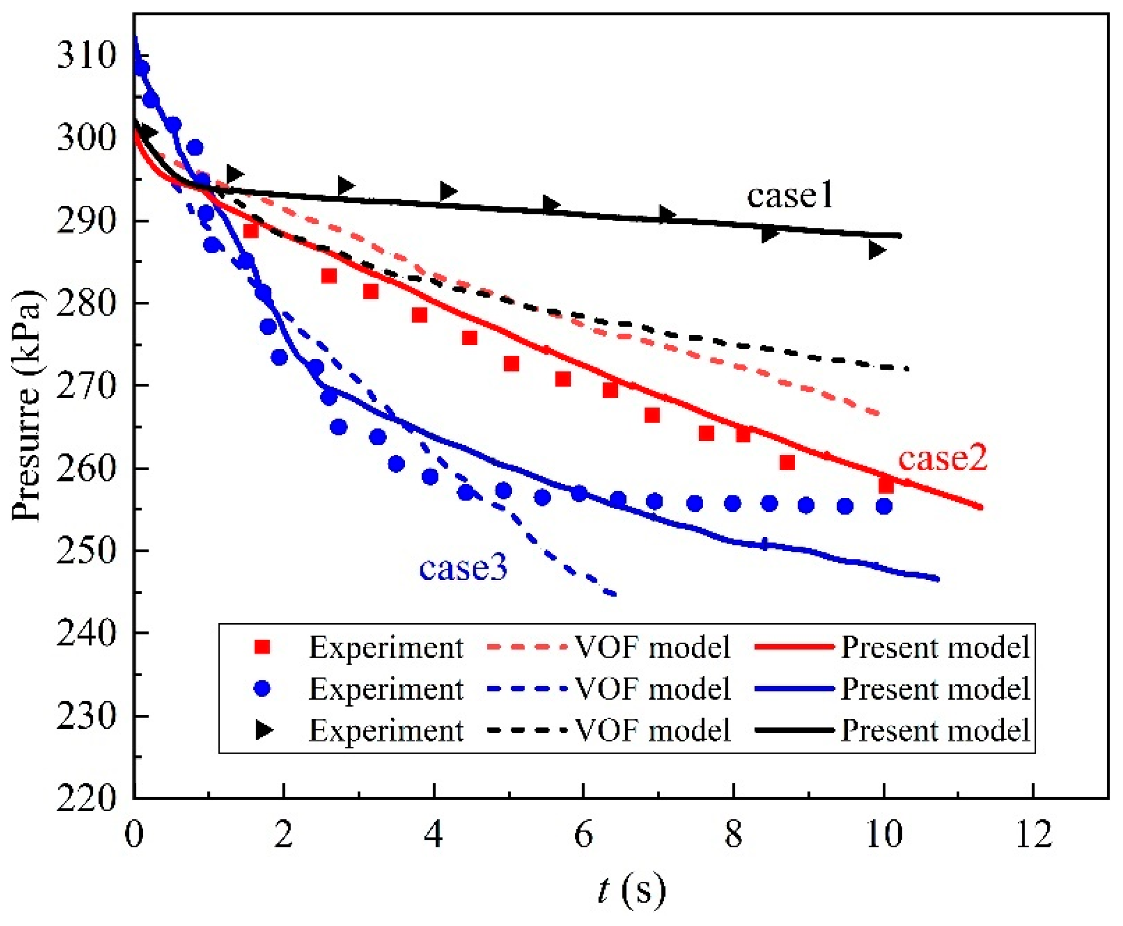
2.6. Validation of CFD Model

In the presented study, the numerical model is validated by comparing it with the liquid sloshing experiments conducted by Grotle et al. [21] and Esoy et al. [33]. The experiments were carried out with a water storage tank mounted on a rotating platform. In the experimental vessel, the midpoint is taken at the bottom of the vessel acting as the rotation center, θ A represents the maximum rotation angle, and f is the rotation frequency. Pressure sensors installed on the top of the test vessel were used to measure the pressure change in the vessel, and a transparent vessel was used for better visualization of morphology. The working fluids of the experiments were water, of which the initial temperature was 393.15 K, and vapor temperature at 406.15 K; thus, the experiments use a condensation process and the pressures of the vapor regions continuously decrease. In the model verification, the geometry model, the working fluid and working conditions were the same as the experiments in order to ensure the consistency of the setting of the simulation cases and the experiments. Figure 4 shows the tank pressure comparison between the numerical results and three experimental cases. The numerical results by Wu and Ju [20], who applied the VOF model and ignored the interfacial drag, are also compared. The comparison reveals that the present model performs a better coincidence against the experimental data. In addition, the simulated flow pattern is satisfactorily consistent with the experimental results, as seen in Figure 5.

3. Results and Discussion

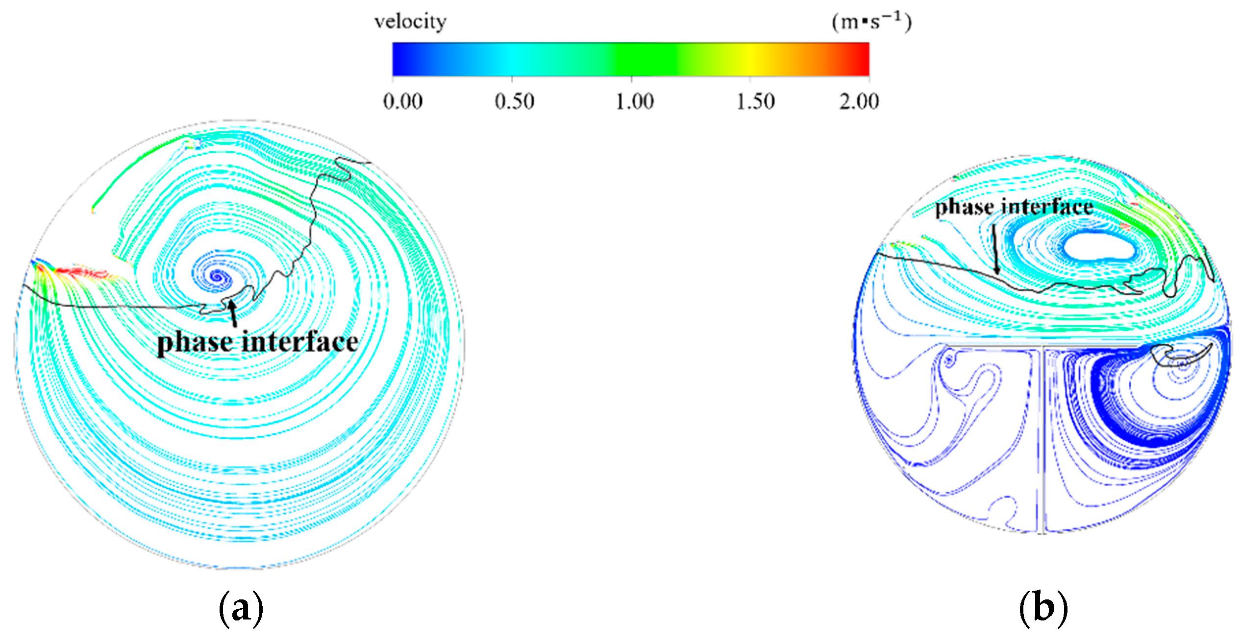
3.1. Interfacial Behaviors

The interfacial behavior with an LR of 50% at various times in a period is shown in Figure 6. Within 0–0.5 s, the liquid sloshes to the left. The sloshing excitation peaks at half a cycle of sloshing (t = 0.5 s) and the liquid reaches to the top wall. Within 0.5–1 s, the liquid sloshes to the right, and the sloshing height is lower than that on the left because the liquid tends to slosh to the left due to inertia, and the tank moves in the opposite direction. A portion of the liquid bulk flows to the right because the direction of rotation of the tank changes, and the liquid on both sides of the tank collides towards the center of the tank when there is a change in sloshing direction. A liquid splash phenomenon occurs in the sloshing process.
The centroid displacements of the liquid tank with different LRs are shown in Figure 7. With the increase in the LR, the displacement of the centroid decreases, and the degree of sloshing decreases. On the one hand, as the volume of the liquid increases and its inertial force increases, which causes the liquid to dissipate more energy due to external work, the degree of liquid sloshing becomes smaller. With the larger LR, the sloshing liquid easily collides with the top of the tank. The top of the tank limits the movement of the liquid, thus reducing the centroid displacement of the sloshing liquid. The impact load on the liquid tank is larger at a low LR.

3.2. Evaporation Characteristics of Liquid Oxygen

Before the sloshing process, the tank keeps quiescent for about 300 s due to the thermal stratification caused by the heat leakage. A free convective boundary layer along the interior surface of the wall is generated. The warmed liquid becomes lighter, and moves upward due to the thermal buoyancy, as shown in Figure 8. After the liquid converges at the center, a small part of the liquid evaporates to move upward, forming small vortices at the interface. Most of the liquid returns at 90° as a downward fluid. The excess heat is not released by surface evaporation, transfers into the core of the liquid, and produces superheated vapors through secondary convection. Simultaneously, almost symmetrical vortices are formed on both sides of the liquid.
The liquid absorbs heat at the interface and near the walls, thus the minimum temperature exists at the core of the liquid region. From Figure 9, it can be observed that the minimum temperature area gradually moves downward. Due to the upward movement of hot vapor, a lot of heat is accumulated at the top of the tank, which results in the formation of a high-temperature zone. Furthermore, part of the vapor is squeezed to flow downward, causing the formation of vortices at the top of the tank. For the vapor region, its minimum temperature occurs at the phase interface. The vapor at the interface flows to the wall under the impetus of the central vortices and fully exchanges heat with the liquid. Figure 10 shows violent surface evaporation at the vapor–liquid interface, and the evaporation rate increases rapidly at the initial stage of static evaporation. At t = 65 s, the evaporation rate rises to the maximum. After that, thermal stratification gradually forms to hinder free convection [1], and the evaporation rate slowly increases under the incessant heat input. At t = 300 s, an elevated temperature is maintained for the complete liquid. According to Figure 10, the evaporation loss of the whole static evaporation process is 1.46 × 10⁻⁴ kg.
The effect of the sloshing frequency on evaporation was studied in detail. To monitor the pressure and temperature changes, three monitoring points were selected in the vapor region. The coordinates of each point are given in Table 3. The data collected at the three monitoring points are averaged to estimate the average pressure and temperature changes.
When liquid suddenly sloshes, the evaporation rate increases rapidly, then drops and stabilizes, as shown in Figure 11. This implies that the convective impedance of surface evaporation suddenly fails and then rapidly restores itself. This phenomenon is called a vapor explosion. The shocking vapor explosions are not dangerous because they are surface evaporation phenomena caused only by the disturbance of the surface layer. According to Scurlock, a surface sublayer which resists evaporation exists at the gas–liquid interface. The molecular evaporation region acts as a weak impedance, whereas the convection region holds a high impedance [34]. The thin and high-resistance region separates the bulk superheated liquid from the surface molecular evaporation region and prevents any severe evaporation.
The intensity of the vapor explosion becomes more apparent when the sloshing frequency increases; however, the most intense vapor explosion is shown by the sloshing liquid bulk when f = 0.8 Hz, and the evaporation rate following the explosion also fluctuates dramatically. This frequency, which falls into the low-frequency band and is lower than the resonant frequency of the tank, is assumed to be similar to the value of the vapor–liquid coupling excitation frequency. One of the generation mechanisms of the vapor–liquid coupling excitation is the collision and impact effect of the liquid slug or the liquid film when the flow is turned; thus, this phenomenon is very likely to occur in the sloshing of the liquid tank. The internal flow excitation of the two-phase flow, which generates the pulse excitation force, can potentially cause the tank to vibrate and damages its structure. Therefore, the natural frequency of the tank should be increased as much as possible to avoid resonance [35]. Moreover, the evaporation rate at a lower sloshing frequency (f = 0.2 Hz and f = 0.5 Hz) gradually reduces after the vapor explosion. For a high sloshing frequency, the evaporation rate increases with time. This is because the high-frequency sloshing destratifies the thermal stratification and the surface impedance is eliminated appreciably, which accelerates the evaporation.
The vapor temperature increases steadily during the static evaporation, as shown in Figure 12. When sloshing starts, the thermal stratification is quickly dissolved and the vapor–liquid starts mixing as the superheated vapor at the top of the tank makes contact with the saturated liquid, which reduces the vapor temperature. As the frequency increases, the temperature drops drastically. Following this, the vapor temperature rises with fluctuations due to continuous input heat. On the other hand, due to the existence of viscosity, the mechanical energy of the sloshing liquid is converted into internal energy, which increases temperature and promotes evaporation. In the vapor–liquid coupling excitation condition, the vapor temperature rises slowly. The explication is that a larger heat exchange area between the steam and the liquid due to a higher degree of liquid fragmentation incurs more heat absorption by the liquid from vapor. When the sloshing frequency is extremely low (f = 0.2 Hz), the temperature drops by a minor extent.
Figure 13 explains the phenomenon of rapid pressure loss. First, the vapor and liquid are squeezed and contacted, then the vapors are cooled by liquid oxygen. A higher sloshing frequency leads to a faster pressure drop and causes an intense vapor–liquid heat exchange, whereas pressure loss results in a lower saturation temperature. Therefore, vapor pressure rises faster after depressurization. The pressure recovery under the excitation conditions is accompanied by fluctuations, and the evaporation of liquid oxygen occurs under different sloshing frequencies as shown in Figure 14. The maximum evaporation loss of the vapor–liquid coupling excitation condition is 0.0272 kg, and the minimum evaporation loss with the lowest sloshing frequency is 2.26 × 10⁻⁴ kg. Sloshing increases the evaporation loss of the liquid oxygen.

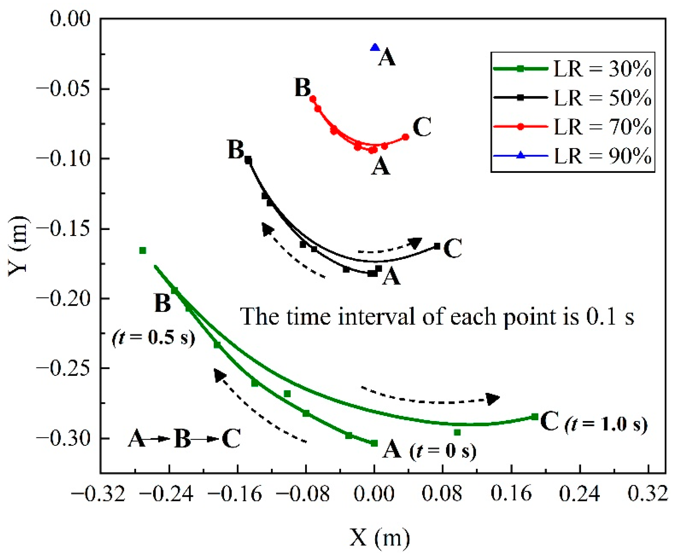
3.3. Anti-Sloshing Performance of T-Shaped Baffle

Baffles with simple structures are preferred to avoid any compatibility issues with the tank design. A T-shaped baffle provides an excellent anti-sloshing effect [28]. In the presented study, a detailed anti-sloshing mechanism was investigated by comparing the cases of no baffle tank with the 50% and 70% LR. The vorticity in the sloshing motion is created by the opposite ends of the baffle, free surface, and tank boundary layers, which can make the fluid move regularly. Figure 15a shows a mild sloshing phenomenon for the 70% LR. The vapor and liquid together form a large vortex and maintain a stable state. It is inferred that the stable vortex can be used as a motion damping factor to reduce the degree of sloshing. Figure 15b shows that the formations of the tip vortices rotate the liquid near the wall around the centers of the vortices, and constantly induce a shearing effect on the wall. Simultaneously, the baffle accelerates the movement of the liquid above it. The combined action of the tip vortices and the shearing effect of the wall cause energy loss, which is not enough to offset the increase in the momentum of the liquid above the baffle, resulting in increased sloshing. As shown in Figure 16a, there is no vortex in the tank with 50% LR, and the fluid movement is irregular. For 0.5LR0.5HR, the liquid is rotated below the baffle, as shown in Figure 16b, which causes energy loss and reduces the liquid momentum. The height of the baffle is the same as that of the liquid level and the complexity of the free surface is strengthened. This phenomenon enhances the interaction between the boundary layer and the free surface and results in enhanced wall shear effects. Based on liquid momentum reduction, the enhanced shearing effect on the wall inhibits movement and reduces the sloshing extent.
As shown in Figure 17a, for 0.5LR0.25HR, the baffle accelerates the liquid above it and does not restrict the liquid movement. The T-shaped baffle enhances the liquid bulk motion above the baffle, which increases the impact on the wall. In 0.5LR0.75HR, the baffle divides the liquid into smaller spaces and small vortices are formed to stabilize the fluid movement in Figure 17c. However, the degree of inhibition is not as good as that of 0.5LR0.5HR. The baffle with an HR of 0.5 provides a superior anti-sloshing effect with 50% LR.
The baffle with an HR of 0.75 has the most obvious sloshing suppression effect when the LR value is equal to 70%, as shown in Figure 18. The vapor and liquid below the baffle form vortices to dampen the motion. On the other hand, a T-shaped baffle divides the inner cavity of the liquid tank into smaller areas, thus the liquid movement is buffered by the wall and baffle in Figure 18c. The liquid bulk above the baffle is accelerated and below the baffle is controlled, but the height of the baffle far beyond the liquid level weakens its control on liquid motion.
Furthermore, the centroid displacement in Figure 19 quantitatively shows the sloshing amplitude with various sloshing conditions. The baffle with an HR of 0.25 shows a negligible effect on the sloshing liquid tank with an LR of 50% and 70%. For the 50% LR, the baffle with an HR of 0.5 reduces the horizontal centroid displacement by 0.13 m and the vertical displacement by 0.08 m within 1 s. In addition, the 0.5HR baffle makes the centroid of the 0.7LR0.5 HR only move to the left. The liquid below the baffle attains a stable state under the restriction of the vortex. Since the vorticity on the right side of the plate is larger, therefore, the motion damping effect becomes stronger, as shown in Figure 18b. The baffle with an HR of 0.75 provides an apparent sloshing suppression effect for the 70% LR, which reduces the horizontal and vertical displacement of the liquid oxygen centroid by 0.06 m and 0.03 m. The 0.75 HR baffle also suppresses the sloshing for the 50% LR. Consequently, the anti-sloshing effect of the T-shaped baffle is determined by the relationship between the height of the baffle and liquid level, which connotes the weight of energy loss and the momentum increment. The energy loss is contributed by the formation of tip vortices and the enhancement of the wall shearing effect. The momentum increment occurs due to the acceleration of the liquid above the baffle.

4. Conclusions

In this study, a 2D sloshing evaporation numerical model was developed by coupling the Eulerian framework and the AIAD method with the consideration of the interphase drag force. The thermodynamic behaviors and the effect of the sloshing frequency on evaporation were discussed. Moreover, based on the anti-sloshing mechanism of the T-shaped baffle, the effects of the baffle height were investigated in detail. The main conclusions of the research include:
(1)
The evaporation rate is significantly promoted once the sloshing condition is imposed. It is attributed to the sharp pressure loss and the conversion of kinetic energy into friction heat.
(2)
Thermal destratification and vapor explosion stimulated by sloshing jointly promote evaporation. The evaporation loss under the vapor–liquid coupling excitation is approximately 120 times that of the evaporation loss under the low-frequency sloshing. This phenomenon may induce structural vibrations and pose a safety hazard.
(3)
The T-shaped baffle behaves with an ascendant anti-sloshing performance when the baffle height approaches the liquid level. The generation of tip vortices and the enhancement of the wall shearing effect contribute to the energy loss and act as the motion damping factors. However, the momentum increment is incurred by the acceleration of the liquid above the baffle. The anti-sloshing performance of the T-shaped baffle is determined by the optimal weight of the energy loss and increased momentum.

Author Contributions

Conceptualization, H.Z. and X.P.; methodology, H.Z. and J.C.; software, H.Z.; validation, H.Z.; formal analysis, H.Z. and X.P.; investigation, H.C., X.G., J.X. and J.C.; resources, H.C., X.G., Q.H. and J.C.; data curation, H.Z. and Q.H.; writing—original draft preparation, H.Z.; writing—review and editing, H.Z., H.C., X.G., X.P., Q.H., J.X. and J.C.; visualization, H.Z. and Q.H.; supervision, X.P., J.X. and J.C.; project administration, H.C., X.G. and J.C.; funding acquisition, J.X. and J.C. All authors have read and agreed to the published version of the manuscript.

Funding

The authors acknowledge the support from the State Key Laboratory of Technologies in Space Cryogenic Propellants (SKLTSCP1507).

Acknowledgments

The computing work in this paper is supported by the public computing service platform provided by the Network and Computing Center of HUST.

Conflicts of Interest

The authors declare no conflict of interest.

References

  1. Duan, Z.; Sun, H.; Cheng, C.; Tang, W.; Xue, H. A moving-boundary based dynamic model for predicting the transient free convection and thermal stratification in liquefied gas storage tank. Int. J. Therm. Sci. 2021, 160, 106690. [Google Scholar] [CrossRef]
  2. Zheng, Y.; Chen, J.; Shang, Y.; Chang, H.; Chen, H.; Shu, S. Numerical analysis of the influence of wall vibration on heat transfer with liquid hydrogen boiling flow in a horizontal tube. Int. J. Hydrogen Energy 2017, 42, 30804–30812. [Google Scholar] [CrossRef]
  3. Wang, Y.; Wang, Z. An overview of liquid–vapor phase change, flow and heat transfer in mini-and micro-channels. Int. J. Therm. Sci. 2014, 86, 227–245. [Google Scholar] [CrossRef]
  4. Davy, G.; Reyssat, E.; Vincent, S.; Mimouni, S. Euler–Euler simulations of condensing two-phase flows in mini-channel: Combination of a sub-grid approach and an interface capturing approach. Int. J. Multiph. Flow 2022, 149, 103964. [Google Scholar] [CrossRef]
  5. Zhang, W.; Ke, P.; Yang, C.; Zhou, C. Progress of computability of multi-scale interface problems in gas-liquid two-phase flow. CIESC J. 2014, 65, 4645–4654. [Google Scholar]
  6. Hoehne, T.; Lucas, D. Numerical simulations of counter-current two-phase flow experiments in a PWR hot leg model using an interfacial area density model. Int. J. Heat Fluid Flow 2011, 32, 1047–1056. [Google Scholar] [CrossRef]
  7. Höhne, T.; Vallée, C. Experiments and numerical simulations of horizontal two-phase flow regimes using an interfacial area density model. J. Comput. Multiph. Flows 2010, 2, 131–143. [Google Scholar] [CrossRef]
  8. Dalla Barba, F.; Scapin, N.; Demou, A.D.; Rosti, M.E.; Picano, F.; Brandt, L. An interface capturing method for liquid-gas flows at low-Mach number. Comput. Fluids 2021, 216, 104789. [Google Scholar] [CrossRef]
  9. Chen, Y.G.; Djidjeli, K.; Price, W.G. Numerical simulation of liquid sloshing phenomena in partially filled containers. Comput. Fluids 2009, 38, 830–842. [Google Scholar] [CrossRef]
  10. Liu, C.; Wang, J.; Wan, D. CFD Computation of Wave Forces and Motions of DTC Ship in Oblique Waves. Int. J. Offshore Polar Eng. 2018, 28, 154–163. [Google Scholar] [CrossRef]
  11. Sanapala, V.S.; Velusamy, K.; Patnaik, B.S.V. CFD simulations on the dynamics of liquid sloshing and its control in a storage tank for spent fuel applications. Ann. Nucl. Energy 2016, 94, 494–509. [Google Scholar] [CrossRef]
  12. Zhao, Y.; Chen, H. Numerical simulation of 3D sloshing flow in partially filled LNG tank using a coupled level-set and volume-of-fluid method. Ocean Eng. 2015, 104, 10–30. [Google Scholar] [CrossRef]
  13. Boniou, V.; Schmitt, T.; Vié, A. Comparison of interface capturing methods for the simulation of two-phase flow in a unified low-Mach framework. Int. J. Multiphase Flow 2022, 149, 103957. [Google Scholar] [CrossRef]
  14. Liu, Z.; Feng, Y.; Lei, G.; Li, Y. Hydrodynamic performance on sloshing process in a liquid oxygen tank under intermittent excitation. Cryogenics 2019, 98, 92–101. [Google Scholar] [CrossRef]
  15. Liu, Z.; Li, C. Influence of slosh baffles on thermodynamic performance in liquid hydrogen tank. J. Hazard. Mater. 2018, 346, 253–262. [Google Scholar] [CrossRef] [PubMed]
  16. Liu, Z.; Li, Y. Thermal physical performance in liquid hydrogen tank under constant wall temperature. Renew. Energy 2019, 130, 601–612. [Google Scholar] [CrossRef]
  17. Liu, Z.; Li, Y.; Zhou, G. Study on thermal stratification in liquid hydrogen tank under different gravity levels. Int. J. Hydrogen Energy 2018, 43, 9369–9378. [Google Scholar] [CrossRef]
  18. Kumar, S.P.; Prasad, B.; Venkatarathnam, G.; Ramamurthi, K.; Murthy, S.S. Influence of surface evaporation on stratification in liquid hydrogen tanks of different aspect ratios. Int. J. Hydrogen Energy 2007, 32, 1954–1960. [Google Scholar] [CrossRef]
  19. Roh, S.; Son, G.; Song, G.; Bae, J. Numerical study of transient natural convection in a pressurized LNG storage tank. Appl. Therm. Eng. 2013, 52, 209–220. [Google Scholar] [CrossRef]
  20. Wu, S.; Ju, Y. Numerical study of the boil-off gas (BOG) generation characteristics in a type C independent liquefied natural gas (LNG) tank under sloshing excitation. Energy 2021, 223, 120001. [Google Scholar] [CrossRef]
  21. Grotle, E.L.; Aesoy, V. Dynamic modelling of the thermal response enhanced by sloshing in marine LNG fuel tanks. Appl. Therm. Eng. 2018, 135, 512–520. [Google Scholar] [CrossRef]
  22. Zuo, Z.; Jiang, W.; Pan, P.; Qin, X.; Huang, Y. Quasi-equilibrium evaporation characteristics of oxygen in the liquid–vapor interfacial region. Int. Commun. Heat Mass Transf. 2021, 129, 105697. [Google Scholar] [CrossRef]
  23. Xue, M.; Lin, P.; Zheng, J.; Ma, Y.; Yuan, X.; Nguyen, V. Effects of perforated baffle on reducing sloshing in rectangular tank: Experimental and numerical study. China Ocean Eng. 2013, 27, 615–628. [Google Scholar] [CrossRef]
  24. Brar, G.S.; Singh, S. An experimental and CFD analysis of sloshing in a tanker. Procedia Technol. 2014, 14, 490–496. [Google Scholar] [CrossRef]
  25. Nayak, S.K.; Biswal, K.C. Fluid damping in rectangular tank fitted with various internal objects—An experimental investigation. Ocean Eng. 2015, 108, 552–562. [Google Scholar] [CrossRef]
  26. Panigrahy, P.K.; Maity, S.U.K. Experimental studies on sloshing behavior due to horizontal movement of liquids in baffled tanks. Ocean Eng. 2009, 36, 213–222. [Google Scholar] [CrossRef]
  27. Akyildiz, H.; Uenal, N.E.; Aksoy, H. An experimental investigation of the effects of the ring baffles on liquid sloshing in a rigid cylindrical tank. Ocean Eng. 2013, 59, 190–197. [Google Scholar] [CrossRef]
  28. Unal, U.O.; Bilici, G.; Akyildiz, H. Liquid sloshing in a two-dimensional rectangular tank: A numerical investigation with a T-shaped baffle. Ocean Eng. 2019, 187, 106181–106183. [Google Scholar] [CrossRef]
  29. Brackbill, J.U.; Kothe, D.B.; Zemach, C. A continuum method for modeling surface tension. J. Comput. Phys. 1992, 100, 335–354. [Google Scholar] [CrossRef]
  30. Marshall, W.R.; Ranz, W.E. Evaporation from Drops—Part I. Chem. Eng. Prog. 1952, 48, 141–146. [Google Scholar]
  31. Ranz, W.R. Evaporation from drops Part II. Chem. Eng. Prog. 1952, 48, 173–180. [Google Scholar]
  32. Lee, W.H. Pressure iteration scheme for two-phase flow modeling. In Mutiphase Transport: Fundamentals, Reactor Safety, Applications, Proceedings of the Multi-Phase Flow and Heat Transfer Symposium-Workshop, Miami Beach, FL, USA 16–18 April 1979; Hemisphere Publishing Corp.: Washington, DC, USA, 1980; pp. 407–432. [Google Scholar]
  33. Grotle, E.L.; Æsøy, V. Numerical simulations of sloshing and the thermodynamic response due to mixing. Energies 2017, 10, 1338. [Google Scholar] [CrossRef] [Green Version]
  34. Scurlock, R.G. Surface Evaporation of Cryogenic Liquids, Including LNG and LPG. In Stratification, Rollover and Handling of LNG, LPG and Other Cryogenic Liquid Mixtures; Springer: Cham, Switzerland, 2016; pp. 41–62. [Google Scholar]
  35. Ma, X.; Tian, M.; Zhang, G.; Leng, X. Numerical investigation on gas-liquid two-phase flow-induced vibration in a horizontal tube. J. Vib. Shock 2016, 35, 204–210. [Google Scholar]
Figure 1. Diagram of the liquid oxygen tank.
Energies 15 06457 g001
Figure 2. Grid schematic diagrams. (a) non-baffle; (b) baffle with HR = 0.25; (c) baffle with HR = 0.50; (d) baffle with HR = 0.75.
Energies 15 06457 g002
Figure 3. Pressure with various mesh numbers.
Energies 15 06457 g003
Figure 4. Comparison of tank pressure (CFD simulation and experimental results) [20]. (Case 1: f = 0.29, θ A = 3°; Case 2: f = 0.40, θ A = 3°; Case 3: f = 0.57, θ A = 3°).
Energies 15 06457 g004
Figure 5. Comparison of interface shape between experimental and simulation results. (a) Case 2; (b) Case 3.
Energies 15 06457 g005
Figure 6. Interfacial behavior at various times in a period (LR = 50%).
Energies 15 06457 g006
Figure 7. Centroid displacements of liquid with different LRs.
Energies 15 06457 g007
Figure 8. Direction of vapor–liquid flow during the static evaporation.
Energies 15 06457 g008
Figure 9. Temperature distribution during the static evaporation. (a) t = 20 s; (b) t = 40 s; (c) t = 120 s; (d) t = 300 s.
Energies 15 06457 g009
Figure 10. The evaporation rate and evaporation loss during static evaporation.
Energies 15 06457 g010
Figure 11. Variation of evaporation rate with different sloshing frequencies.
Energies 15 06457 g011
Figure 12. Vapor temperature with different sloshing frequencies.
Energies 15 06457 g012
Figure 13. Variation of vapor pressure under different sloshing frequencies.
Energies 15 06457 g013
Figure 14. Dynamic evaporation loss under different sloshing frequencies.
Energies 15 06457 g014
Figure 15. Flow diagram with T-shaped baffle vs. non-baffle (LR = 70%, t = 1 s). (a) non-baffle; (b) baffle with HR = 0.5.
Energies 15 06457 g015
Figure 16. Flow diagram with T-shaped baffle vs. non-baffle (LR = 50%, t = 1 s). (a) non-baffle; (b) baffle with HR = 0.5.
Energies 15 06457 g016
Figure 17. Flow diagram of liquid velocity with T-shaped baffle (LR = 50%, t = 1 s). (a) baffle with HR = 0.25; (b) baffle with HR = 0.5; (c) baffle with HR = 0.75.
Energies 15 06457 g017
Figure 18. Flow diagram of liquid velocity (LR = 70%, t = 1 s). (a) baffle with HR = 0.25; (b) baffle with HR = 0.5; (c) baffle with HR = 0.75.
Energies 15 06457 g018
Figure 19. Centroid displacement with various LR values and HR values. (a) non-baffle; (b) baffle with HR = 0.25; (c) baffle with HR = 0.5; (d) baffle with HR = 0.75.
Energies 15 06457 g019aEnergies 15 06457 g019b
Table 1. Simulation cases.
No.CaseLRType of BaffleHRNo.CaseLRType of BaffleHR
10.5LR50%none-60.7LR70%none-
20.5LR0.25HR50%T-shaped0.2570.7LR0.25HR70%T-shaped0.25
30.5LR0.5HR50%T-shaped0.5080.7LR0.5HR70%T-shaped0.50
40.5LR0.75HR50%T-shaped0.7590.7LR0.75HR70%T-shaped0.75
50.9LR90%none-100.3LR30%none-
Table 2. Initial thermophysical properties of the saturated oxygen.
Materials Density   k g ·   m 3 Specific   Heat   Capacity   J   ( kg × K ) 1 Thermal   Conductivity   W × ( m × K ) 1 Dynamic   Viscosity   k g · ( m × s ) 1 Thermal   Expansion   Coefficient   ( K ) 1
Oxygen-liquid1127.11707.90.146771.8 × 10−40.0045085
Oxygen-vapor5.802975.90.008477.2 × 10−60.0121
Table 3. Coordinates of pressure monitoring points.
MonitorCoordinatesMonitorCoordinatesMonitorCoordinates
P1(0, 0.215)P2(0.2, 0.215)P3(−0.2, 0.215)
Publisher’s Note: MDPI stays neutral with regard to jurisdictional claims in published maps and institutional affiliations.

