The Railway Timetable Evaluation Method in Terms of Operational Robustness against Overloads of the Power Supply System

Abstract

The main aim of this study was to develop a method for assessing the level of robustness of timetabled transport performance in rail transport. When the railway lines are supplied by DC networks, lower voltages are observed, and consequently, current values are often ten times higher than in AC networks. This is an operational problem, as high currents make it easier to overload the supply network. Based on a literature review, the authors show that the problem of running railway traffic when the capacity of the power supply network is limited (by the size of the permitted currents) is not well studied. The authors propose a method based on the Markov approach supplemented by classical theoretical vehicle traffic dynamics to improve the operational robustness of the rail transport system using DC power supply system. Each train run was parameterised in such a way that it is possible to determine the state that the train is in during the run, the transitions between states, and the determination of the probabilities of occurrence of such states. On the other hand, classical vehicle dynamics was used to assess the load generated by the train on the power grid. The proposed method—reduced to a function—was verified using a case study. The method of timetable reconfiguration proposed by the authors increased the operational robustness from 0.9454 to 0.9774.

1. Introduction

The most common consequences of unwanted events in the railway system are delays and other disruptions caused by them. Approximately 98% of all undesirable events on the railway are classified as safe. Nevertheless, such small consequence events can cause the occurrence of other more significant events such as via the domino effect. Because of delays or general disruptions, the theoretical schedule cannot be implemented (as a deviation in time and space). The resulting changes destroy the planned operation schedule.

Consequently, the scheduled train traffic without collisions and direct interactions between trains is lost. For example, traffic disruptions can lead to an aggregation of trains on an energy supply section and consequently cause an overload of the equipment with further damages and traffic consequences. Therefore, this paper aimed to elaborate on a solution for evaluating the timetables in terms of overloads and robustness against them.

The contribution is built on six chapters, including the introduction and conclusions. The literature research shows that the gap filled by this contribution and the starting level in terms of approaches and concepts. This is followed by chapter three, which describes the energetical basics and assumptions necessary for the evaluation. Chapter four describes the evaluation method, while the following chapter shows a railway case study. Finally, chapter six ends the paper with conclusions.

2. Literature Review

The problem of the energy demand in rail transport for electricity has been addressed by numerous researchers, as confirmed by some review papers [1,2], wherein the authors have collected dozens of works on the subject. Solutions to reduce the energy intensity of the system, including through the implementation of energy-efficient train driving techniques, are frequently mentioned in previously published works. Researchers are proposing different approaches: using coasting to save on energy in cases where automatic train operation systems are implemented [3] or a precise train driving strategy [4], trajectory optimisation using microsimulation [5], implementing the Ant Colony Algorithm for train scheduling using the traveling salesman problem [6] or graph theory [7], coordination between trains changing drive modes [8], using line slopes to save energy [9], or changing the trajectory of an existing timetable train using the time margin [10]. Such train driving strategies are highly desirable for railway operators. They are usually applied when the operating schedule of the rail transport system is homogeneous, that is, when vehicles of the same type are used on the network or when there are many repetitive traffic situations: the freight line with long slope [9] or homogeneous, autonomic traffic in the metro system [11]—the metro system was also considered in [12,13], wherein synchronisation between trains was proposed. The authors proposed modifying stop times in stations to synchronise train modes and transfer energy between trains. Supporting accelerated trains with energy from synchronised braking trains was also proposed in [5,14,15]. These measures aim to use the braking energy of one train to accelerate another train, thereby reducing the energy demand on the country’s electricity grid. The energy intensity of the planned schedule was also investigated to check the possibility of recovering braking energy and using it for traction. Here, publications have predominantly proposed one of three basic approaches: (a) directly transferring the energy recovered from the braking process to the acceleration of another train on the railway line using the overhead line; (b) installing an energy store (usually a supercapacitor) on the vehicle that stores the energy recovered during braking and gives it back during the subsequent switching on of the traction motors—with supercapacitors in metro trains [16] or a hybrid accumulation system directly installed onboard [17,18]; and (c) rebuilding the power supply network to create global energy stores that take the energy given to the overhead line by braking trains and give it back in a trailing manner as required: the energy is immediately used by another vehicle [19]; electricity is returned to the grid or stored in energy storage tanks (ESSs) [20]; the energy recovered from a braking vehicle is used to accelerate the other one in the example of an urban railway network [21]; and energy is transferred between paired trains [22]. The third group of approaches to considering the rail transport system’s energy intensity relates to permissible capacity issues on the power supply network [12,22]. Such problems are relevant when using DC power systems with relatively low voltages (0.75 kV DC, 1.5 kV DC, 3.0 k V DC) compared to AC power systems. In the case of timetabled operation, the permissible load capacity is considered at the timetable construction stage. As such, the research undertaken to date [23,24,25,26] has discussed the issue of the long-term strategic decision-making process for the railway transport system and the detailed business planning process. However, the rail transport system disruptions and train movements do not follow a pre-planned timetable. It is therefore necessary to plan the use of the rail transport system so that it can withstand the effects of deviations from the timetable. In the context of energy consumption, the robustness of the rail system can be considered as the ability to carry out train services, i.e., not to exceed the permissible load on the supply system. The incorrect implementation of the timetable is associated with the occurrence of delays. A flexible timetable structure allows train delays to be minimised. This is a crucial issue during timetable evaluation [27,28,29]. Due to the use of high-speed circuit breakers in the mains, which react by disconnecting the power supply when the permissible load indications of the electrical substation are exceeded, the system’s robustness should be verified at the critical point. This approach was used in [30] and the application shows an optimisation method: ex-post evaluation using microscopic simulation. Such an action aims to understand the increase in robustness at the critical point.

Previous work has used Markov approaches for train scheduling, but not in the context of increasing the robustness of the system against network overload, for example, the states of moving trains are used in [31] to a variable-speed model for the timetable rescheduling problem or in [32] to specify the delay distribution in train schedules.

Based on the performed review of the state of the art, it is possible to conclude that the energy intensity of the rail transport system has been widely addressed. Researchers have pointed to opportunities for the rational use of recoverable energy and indicated the conditions and constraints for power supply networks. They have also addressed the robustness of the rail transport system, including the occurrence of disturbances and pointed to measures to minimise their effects. This work defines an assessment of schedule robustness to disruption. However, a gap was perceived in the absence of a comprehensive study on robustness in the context of power supply network loads under disturbed traffic conditions. In this paper, the authors attempted to do so.

3. Physical Description of Train Movement

The capacity of a railway line can be limited not only by the physical occupation of the railway track by a train, but also by the load on the power supply network caused by the trains on the system. This limitation is especially relevant for power supply systems with a relatively low—for railway realities—voltage, including the 3 kV DC power supply system. In the case of trains equipped with the most powerful engines, it is necessary at the timetable construction stage to verify whether the scheduled traffic overloads the electrical substations. However, in the case of disrupted traffic implemented with deviations from the timetable, electrical substations can also be overloaded. This is facilitated by the frequent stopping of trains caused by a train waiting for a section of the railway line to be cleared by another train moving ahead.

The current load on an electrical substation by a passing train is primarily defined by the power at which the traction motors are currently operating:

$$I=\frac{P}{U}$$

(1)

It is known that the formula for the power with which the traction engines of a train operate takes the form:

$$P=F·\frac{dx}{dt}$$

(2)

where: F—tractive effort; x—distance; and t—time.

The value of the traction force generated by the traction motors is also known. Its value for the train is obtained by solving the equation of motion of the train, based on Newton’s second law of dynamics [33,34]:

$$F\left(v,x\right)=m·k·\frac{d^{2}x}{d{t}^2}$$

(3)

where: m—the mass of train; and k—coefficient of swirling mass.

The value of the tractive effort varies as a function of velocity and distance. Moreover, it depends on the driving mode that the train is in. There are four primary driving stages for each train [35]. The acceleration mode (mode ‘a’, Equation (4)) aims to increase the train’s velocity. Acceleration consists of two phases: starting (from standstill to a certain limiting speed—phase ‘a₁’) and accelerating (further increasing velocity—phase ‘a₂’) [35]. These phases use different parts of the traction characteristics in the vehicle. The constant-speed running mode (mode ‘b’) involves overcoming resistance to motion to maintain a uniform crossing speed (Equation (5)) [34]. Coasting mode (mode ‘c’) consists of running the train with the traction motors switched off [5,34]—the balance of forces is described in Equation 6. Braking mode (mode ‘d’) involves applying the brakes and reducing the running speed (Equation (7)) [34]. In Equations (6) and (7), there is no component involved in traction effort. This means that there is no energy consumption for traction purposes in the coasting and braking modes. For this reason, only three states will appear in the remainder of this work: the generalised acceleration state (1); the constant-speed running state (2); and the state in which the train does not consume energy for traction purposes (3).

F(v,x) = Z(v) − W(v)−I(x)

(4)

F(v,x) = 0, Z(v,x) = W(v) + I(x)

(5)

F(v,x)= –W(v) − I(x)

(6)

F(v,x) = B(v) + W(v) + I(x)

(7)

where: Z—tractive effort; B—braking force; W—movement resistance force; and I—resistance forces depending on the tenor of the railway line.

Graphically, the driving modes are presented in Figure 1 in the form of interconnected graphs showing (as a function of distance) the effect of varying the driving force on the speed of the train and its instantaneous energy intensity.

Due to the relatively small speed range in which phase a₁ is used and the resulting short start-up time, it can be assumed that, with only a slight simplification, the current consumption is the same for the entire phase ‘a’ and that it takes on a constant value. This is, moreover, the law in the case of the use of resistance control, which is commonly used in vehicles that are several decades old and still in use today.

Combining Equations (1)–(3) gives the relationship between the current value measured at the primary circuit of the traction vehicle and the train movement parameters:

$$I=\frac{m·k·\frac{d^{2}x}{d{t}^2}·\frac{dx}{dt}}{U}$$

(8)

In addition to the traction purposes, other components and apparatus installed on the vehicle must also be powered. These include vehicle heating/air-conditioning, lighting, the powering of electrical sockets in the carriages, the heating of water in the toilets, communication equipment installed in the rail vehicle, automation systems related to train safety, on-board computer, compressors for maintaining pressure in the primary and auxiliary lines, and inverter.

The increased load on the electricity network also generates losses between the wheel–rail contact and the entrance to the electrical substation. The efficiencies of such assemblies and system components must be considered in this case, in particular: η₁—efficiency counting other energy consumption, e.g., to the power apparatus located in locomotive or cars (0.96); η₂—efficiency counting the train’s interior heating (0.93); η₃—efficiency of contact line (0.91); η₄—efficiency counting the aberrant movement work (0.98); and η₅—efficiency of an electricity substation (0.94) [33,36]. This is a simplifying approach, but one that can be applied when aggregating the train movement parameters to several states in which the train resides. Therefore, Equation (8) should be expanded to the following form:

$$I=\left(\frac{m·k·\frac{d^{2}x}{d{t}^2}·\frac{dx}{dt}}{U}+I_{nt}\right)·\frac{1}{{\eta }_1}·\frac{1}{{\eta }_2}·\frac{1}{{\eta }_3}·\frac{1}{{\eta }_4}·\frac{1}{{\eta }_5}$$

(9)

where: I_nt—current drawn by the train for non-traction purposes.

4. Method Description

The presented approach, the used assumptions, and the definitions based on the research work of the authors. A more detailed understanding of the helpful basics referring to robustness and its calculation can be found in the papers [37,38,39,40]. Operational robustness is related to the processes implemented by the socio-technical system. It can be defined as the ability to compensate for process disruptions by designing the process schedule. Thus, a fully operational robust system has no disruptions in process implementation after system unavailability, without any reconfiguration actions. Operational robustness is analysed for a pair of processes, as the probability $Pr\left(\mathsf{\Delta }{T}_{\alpha }\le T_{\beta }^{\alpha }\right)$ that the time deviation $\mathsf{\Delta }{T}_{\alpha }$ of process $\alpha$ from the shortest implementation time $min{T}_{\alpha }^{dur}$ will be no higher than the time–space $T_{\beta }^{\alpha }$ between processes $\alpha$ and $\beta$. Thus:

$$OR{o}_{\beta }^{\alpha }=Pr\left(\mathsf{\Delta }{T}_{\alpha }\le T_{\beta }^{\alpha }\right)={\mathrm{F}}_{\alpha }\left(T_{\beta }^{\alpha }\right)=\underset{0}{\overset{T_{\beta }^{\alpha }}{{\displaystyle \int }}}{f}_{\alpha }\left(\mathsf{\Delta }{T}_{\alpha }\right)d\left(\mathsf{\Delta }{T}_{\alpha }\right)$$

(10)

where: $OR{o}_{\beta }^{\alpha }$—operational robustness for processes α and β; $f_{\alpha }\left(\Delta T_{\alpha }\right)$—probability distribution of the time deviation $\mathsf{\Delta }{T}_{\alpha }$ of process $\alpha$ from the shortest implementation time $min{T}_{\alpha }^{dur}$; ${\mathrm{F}}_{\alpha }\left(T_{\beta }^{\alpha }\right)$—cumulated distribution function for $\mathsf{\Delta }{T}_{\alpha }=T_{\beta }^{\alpha }$; meanwhile, the distribution $f_{\alpha }\left(\mathsf{\Delta }{T}_{\alpha }\right)$ is shown in Figure 2.

The operational robustness against overloads is the ability of the system to prevent overload situations only involving process resources. Thus, an appropriate process structure and time reserves are sufficient to compensate for consequences, and reconfiguration is not necessary to prevent overloads. Operational robustness against overloads can be quantified by the probability that no overload situation will occur:

$$OR{o}_{overload}^g={\displaystyle \prod }_{j=1}^{J}OR{o}_{overload}^{j|g}={\displaystyle \prod }_{j=1}^J\left(1-OV{u}_{overload}^{j|g}\right)$$

(11)

where: $OR{o}_{overload}^g$—operational robustness against overloads; $J$—number of identified aggregated traffic train groups; $OR{o}_{overload}^{j|g}$—operational robustness against overloads of j-th train group on section g; $OV{u}_{overload}^{j|g}$—operational vulnerability to overloads of the j-th train group on section g.

The aggregated train traffic groups are identified based on the trains’ cumulated current, where the trains are analysed one after the other in the order resulting from the schedule. A given set of trains is classified as a group if their cumulated maximum current exceeds the limit of the section:

$$I_{cum}^{j|g}={\displaystyle \sum }_{i=\alpha }^{\omega }{I}_{max}^{i|g} \underset{I_{cum}^j}{\overset{{\displaystyle \bigvee }}{}} {\displaystyle \sum }_{i=\alpha }^{\omega -1}{I}_{max}^{i|g}\le I_{max}^g \wedge {\displaystyle \sum }_{i=\alpha }^{\omega }{I}_{max}^{i|g}>I_{max}^g$$

(12)

where: $I_{cum}^{j|g}$—cumulated maximum current for train group j on section g; $I_{max}^{i|g}$—the maximum current created by train i on section g; $I_{max}^g$—cumulated maximum current for section g; and $\alpha , \omega$—the first and the last train of group j, respectively.

Operational vulnerability to overloads is the opposite quality of operational robustness. For the j-th train group, a probability measure can be represented calculated according to the formula:

$$OV{u}_{overload}^{j|g}=P_{\mathsf{\Delta }}^{\alpha |\omega }\cdot P_{sch}^{\omega }\cdot P_{Imax}^{j|g}$$

(13)

where: $P_{\Delta }^{\alpha |\omega }=Pr\left(\mathsf{\Delta }{T}_{\alpha }\ge T_{\omega }^{\alpha }-T_{min}^{\beta }\right)$—the probability that the first train $\left(\alpha \right)$ of the aggregated train group will be delayed $\left(\mathsf{\Delta }{T}_{\alpha }\right)$ at least so that the time–space between the first $\left(\alpha \right)$ and last train $\left(\omega \right)$ of the group will be consumed (excluding the minimum time–space $\left(T_{min}^{\beta }\right)$ necessary for all trains between the first and last to pass the given section); $P_{sch}^{\omega }=Pr\left(\mathsf{\Delta }{T}_{\omega }=0\right)$—the probability that the last train $\left(\omega \right)$ of the group will be punctual; and $P_{Imax}^{j|g}$—the probability that the j-th train group will reach the maximum current on section g.

The probability of a maximum current occurrence for a given train group on a given section is calculated as the product of probabilities that each train in the group on the section will use the maximum current.

$$P_{Imax}^{j|g}=\mathrm{Pr}\left({\displaystyle \sum }_{i=\alpha }^{\omega -1}{I}_{max}^i\le I_{max}^g \wedge {\displaystyle \sum }_{i=\alpha }^{\omega }{I}_{max}^i>I_{max}^g\right)={\displaystyle \prod }_{i=\alpha }^{\omega }{P}_{Imax}^{i|g}$$

(14)

where: $P_{max}^{i|g}$ is the probability that the i-th train will reach the maximum current on section g. The scheduled and disrupted trains are considered separately because of unscheduled stops, and the energy consumption will increase.

The scheduled and disrupted trains are separately considered because:

$$P_{max}^{i|g}=P_{1|sch}^{i|g}·P_{sch}^{i|g}+P_{1|dis}^{i|g}·P_{dis}^{i|g}$$

(15)

where: $P_{1|sch}^{i|g}$—the probability that train $i$ will be in a state of maximum current load for a scheduled situation on section g; $P_{sch}^{i|g}$—punctuality, the probability that train $i$ will be punctual on section g; $P_{1|dis}^{i|g}$—the probability that train $i$ will be in a state of maximum current load for a disrupted traffic situation on section g; and $P_{dis}^{i|g}$—the probability that train $i$ will be disrupted on section g.

The separation of these two situations is caused by considering the best-case scenario (there are only stops and accelerations resulting from the schedule) and the worst-case scenario (additional unscheduled stops due to a changing traffic situation), examples of which are shown in Figure 3 and Figure 4, respectively.

The $P_{1|sch}^{i|g}$ and the $P_{1|dis}^{i|g}$ probability for one train will be calculated using a state-transition model solved by the Markov approach. For a general situation, the graph model was elaborated, as shown in Figure 5. The Markov approach is most often used for reliability and operation process analysis. The qualities of this approach are described in terms of the railway system, for example, in [41]. According to the qualities, the modelling method fits the problem of determining the probability of a maximum current situation.

The shown state-transition model consists of three states and six possible transitions. State one represents the acceleration phase, first with the constant traction force and then the constant power. State two represents the phases in which the vehicle drives at a constant speed. The infrastructure characteristics can be considered as the almost maximum current situation or lower current level. The present study assumes that the current level for state two is significantly lower than the maximum one. Finally, state three represents the situation in which the energy consumption is at the minimum level during braking, driving without traction or standing in stations (Figure 6).

Three differential equations describe the model:

$$\{\begin{array}{c}{P^{\prime }}_1\left(t\right)=-\left({\lambda }_{12}+{\lambda }_{13}\right)·P_1\left(t\right)+{\lambda }_{21}·P_2\left(t\right)+{\lambda }_{31}·P_3\left(t\right)\\ {P^{\prime }}_2\left(t\right)={\lambda }_{12}·P_1\left(t\right)-\left({\lambda }_{21}+{\lambda }_{23}\right)·P_2\left(t\right)+{\lambda }_{32}·P_3\left(t\right)\\ {P^{\prime }}_3\left(t\right)={\lambda }_{13}·P_1\left(t\right)+{\lambda }_{23}·P_2\left(t\right)-\left({\lambda }_{31}+{\lambda }_{32}\right)·P_3\left(t\right)\end{array}$$

(16)

where: $P_1\left(t\right)$—the probability of being in the maximum current state; $P_2\left(t\right)$—the probability of being in the current intermediate state; $P_3\left(t\right)$—the probability of being in the minimum current state; and ${\lambda }_{12},\dots ,{\lambda }_{32}$—transition intensities between states 1 and 2, 2 and 3, etc.

Introducing the standardisation formula that all probabilities must give the sum of one and the assumption of stationarity because of the time reaching infinity, the stationary probability of maximum current is given by the formula:

$$P_1=\frac{{\lambda }_{21}{\lambda }_{32}+{\lambda }_{21}{\lambda }_{31}+{\lambda }_{23}{\lambda }_{31}}{{\lambda }_{12}{\lambda }_{23}+{\lambda }_{12}{\lambda }_{32}+{\lambda }_{12}{\lambda }_{31}+{\lambda }_{21}{\lambda }_{32}+{\lambda }_{21}{\lambda }_{31}+{\lambda }_{21}{\lambda }_{13}+{\lambda }_{23}{\lambda }_{31}+{\lambda }_{23}{\lambda }_{13}+{\lambda }_{32}{\lambda }_{13}}$$

(17)

The proposed method using the above-explained knowledge consists of seventeen steps, from data analysis to a synthetical estimation of the operational robustness measure. A general view is shown in Figure 7.

Step 1.

The infrastructure parameters are analysed using available databases, and data are gathered for calculations. The minimum data needed for further analyses are the speed limits, the longitudinal profile, the curves, the energy section locations, and the maximum current available.

Step 2.

The second step is based on the parameter identification process. The scheduled train speeds are identified from the planned timetable, mainly the intermediate stops.

Step 3.

Using the operational database, the delay probability density function is estimated for the train in the given section.

Step 4.

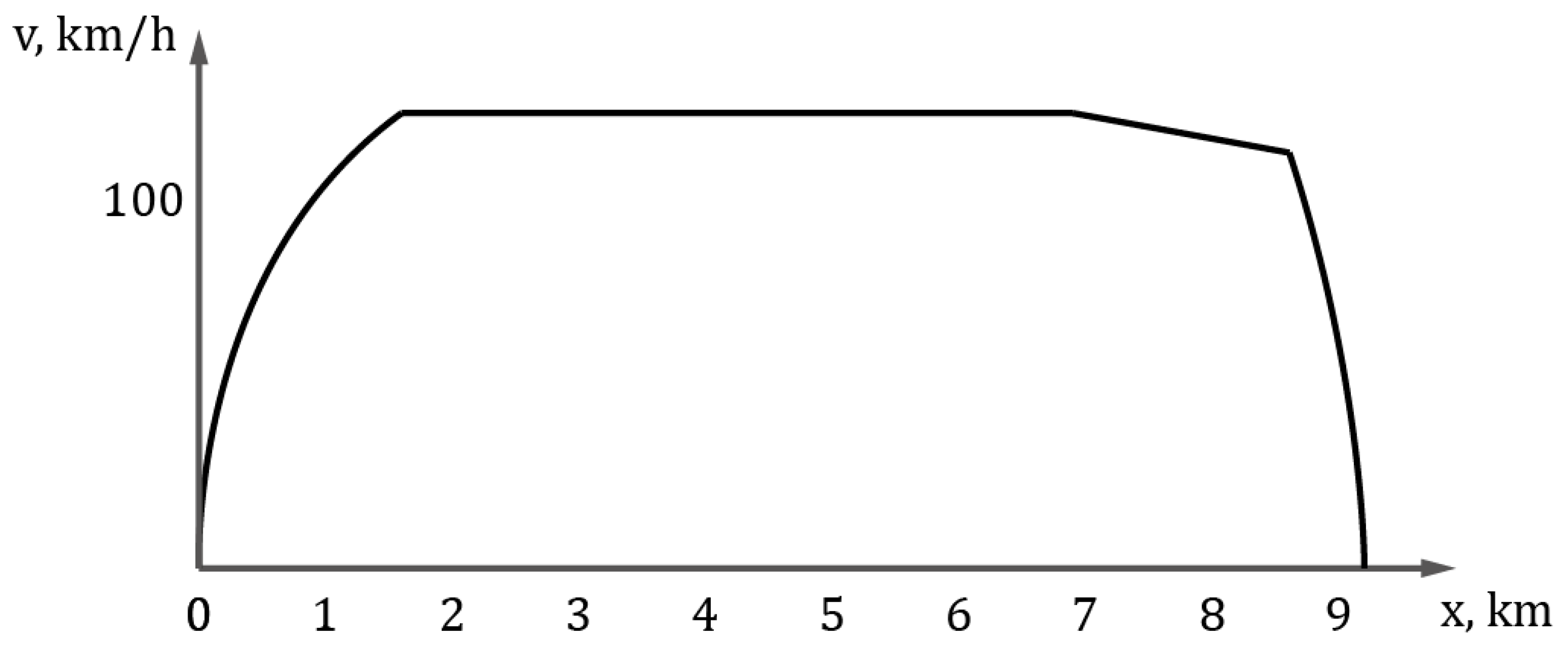
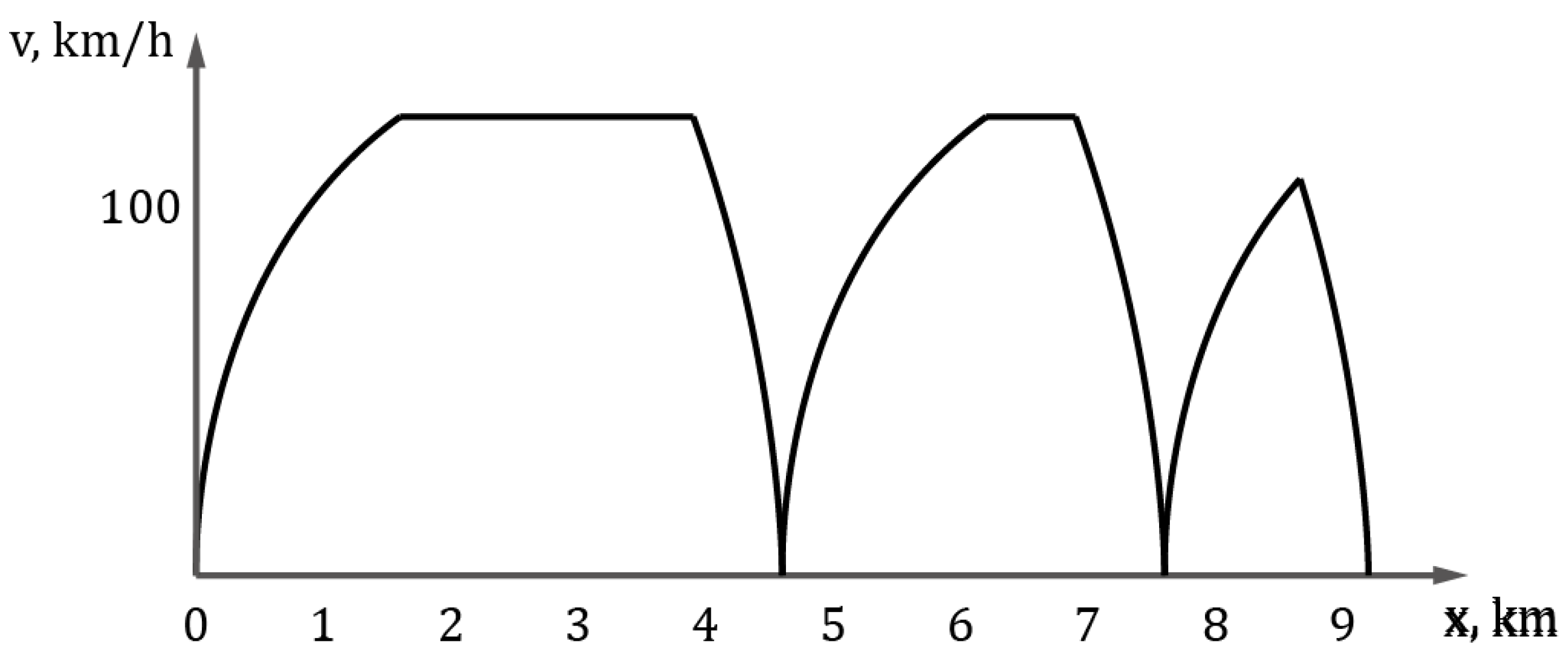
Using the gathered data on infrastructure and timetable, the equation of motion is solved for the analysed section and the first train for a scheduled traffic situation.

Step 5.

This step finds the maximum current for a given train on the section.

Step 6.

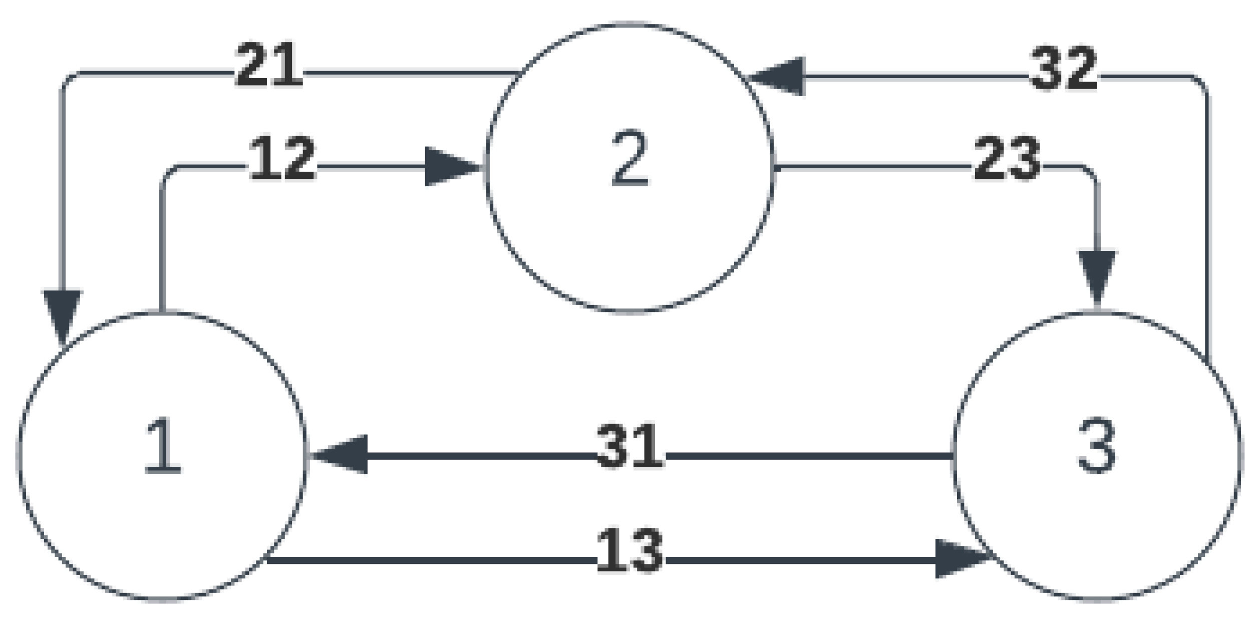
Simplifying the equation of motion results in a discrete form of current vs. time form: state vs. time, where all current values are translated into one of three possible current-dependent states (maximum, intermediate, and low).

Step 7.

The times between states are extracted from the state vs. time graph to calculate the mean time between the transition from one state to another. Then, the inverse values of the mean times between the states are calculated to obtain the transition intensities between these states.

Step 8.

According to the Markov model and the final formula (17), the probability of maximum current occurrence is calculated for the given train on the given section. The probability estimation is performed for the scheduled operation for the first iteration.

Step 9.

Step 9a. The decision is made depending on whether the estimation was performed for the scheduled operation or disrupted traffic. If it was for scheduled operation, the algorithm moves to step 8a. If not, then it moves to step 10.

Step 9b. During this step, the third one is repeated for the disrupted scenario, and the algorithm continues from step 5.

Step 10.

According to formula (15), the maximum current probability occurrence for the given train on the given section (including disrupted and scheduled situations) is calculated.

Step 11.

The decision depends on whether the train is the last one to analyse. If so, then the algorithm moves on to step 12. If not, then it moves back to step 3.

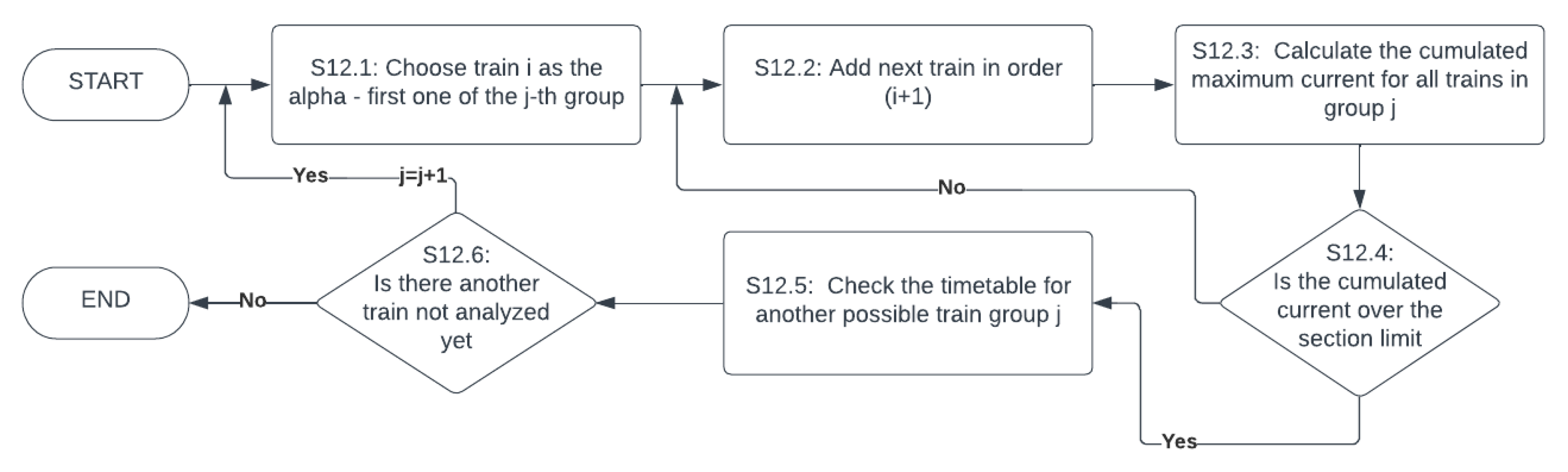
Step 12.

In this step, train groups are built. Starting from the first train in the schedule, the trains are grouped together until the maximum current on the section is exceeded by their cumulated maximum current. Step is described as a Figure 8.

Step 13.

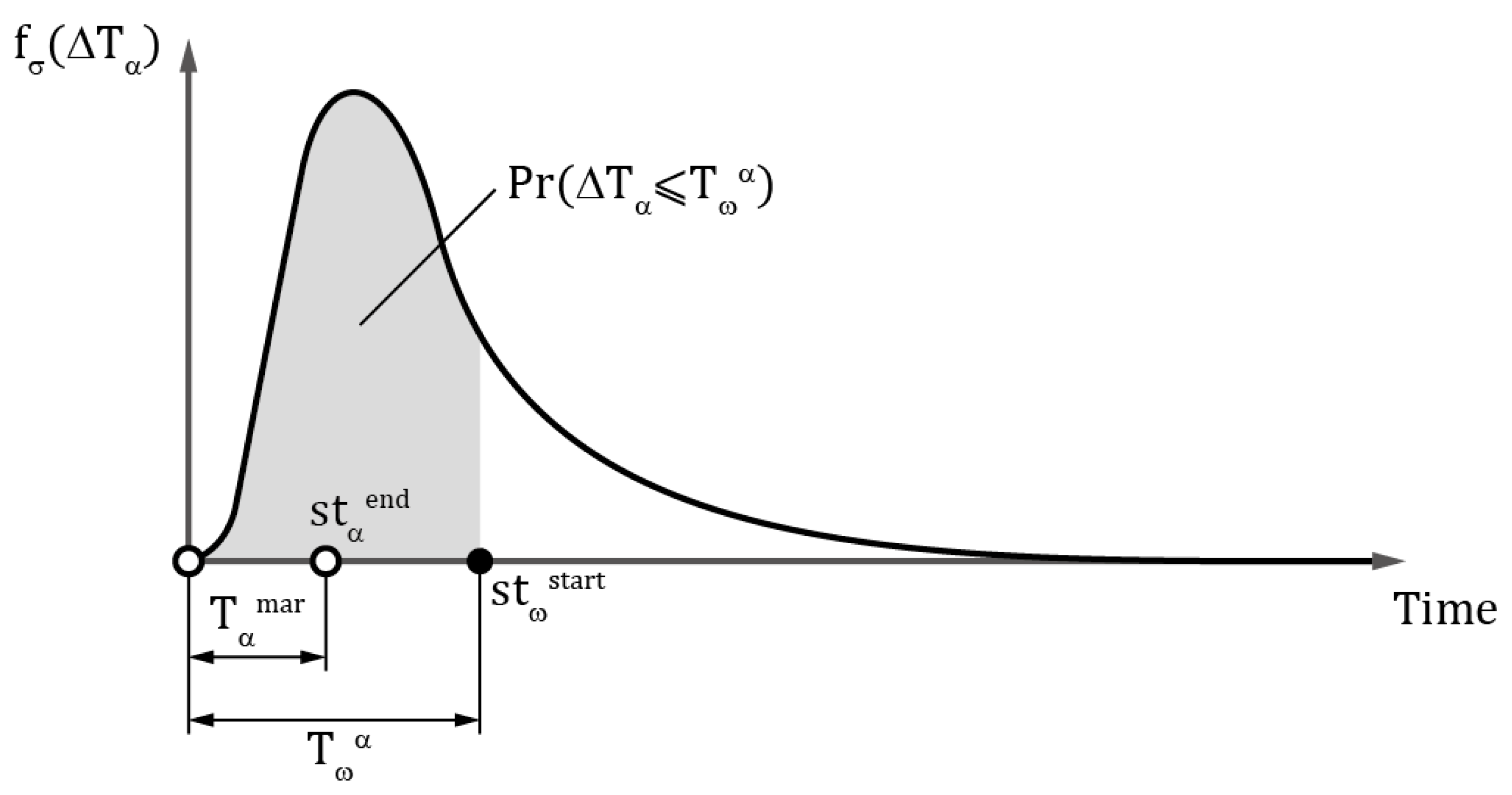
Based on the estimated delay probability functions in step 10, the probability that train alpha will aggregate the group by being late and the probability that the omega train in the group will be on time are calculated. Their product gives the probability that the j-th group will occur. After multiplying them by the probability that the maximum current will occur (Equation (14)), we obtain the probability that the j-th group will cause an overload (Equation (13)).

Step 14.

It is analysed whether group j is the last one. If not, the algorithm moves back to step 13 to calculate the overload probability for the next aggregated group in the section.

Step 15.

According to Equation (11), the final measure of robustness against overloads is calculated.

Step 16.

If there is no other section to analyse, the algorithm ends.

5. Case Study

The method proposed in this paper was verified through the example of a section of railway line with mixed passenger and freight traffic. Below, the results of the given steps are explained according to the previous paragraph.

Step 1. and Step 2. A section of railway line consisting of three feeder sections—with lengths of 9.9, 9.2, and 11.6 km, respectively, was considered. The sections are fed on both sides from two feeder substations of 4 MW each, with one substation feeding two adjacent feeder sections. The boundaries of the supply sections are located within the substations. The railway line is equipped on the routes between the stations with automatic line interlocking, increasing the line’s capacity.

Two types of trains run on the railway line under consideration. The first type is the four-member electric multiple units (EMUs) with a total traction motor power of 2.4 MW, and a permitted running speed of 160 km/h; however, due to the limitation of the permitted velocity due to the one-person traction team, they run at a speed not exceeding 130 km/h. In addition, these trains generate an average non-traction current consumption of 32.9 A. These trains run on passenger services with scheduled stops at stations. They have priority over freight trains.

Freight trains with an average weight of 2.2 Gg are run with 5 MW electric locomotives. They run at speeds not exceeding 80 km/h. They are halted only when necessary. The auxiliary equipment installed on the trains generates an average non-traction current consumption of 24.3 A.

The rail system’s use schedule for approximately three hours was analysed. A total of 32 trains were identified, including 18 passenger trains (9 connections in the “there” direction and 9 in the “return” direction) and 14 freight trains (7 trains in each direction). The figure shows the timetable as a traffic diagram (Figure 9).

Due to the need to maintain technical times, freight trains often have to make additional stops even though the railway line is equipped with automatic line interlocking. The track occupation on the railway track would not determine such a necessity. In practice, line interlocking is used when a slower (generally freight) train is followed by a faster (passenger) train. However, this involves an increase in the running time of the passenger train due to the need to wait for the preceding train to clear the gap.

Step 3. Using the operation database on undesirable events, the basic probability qualities were estimated for the given section and types of trains. The results are shown in

Table 1. The results of estimations of probability qualities.

Train Type	${\mathit{P}}_{\mathit{s}\mathit{c}\mathit{h}}^{\mathit{i}|\mathit{g}}$	${\mathit{P}}_{\mathit{d}\mathit{i}\mathit{s}}^{\mathit{i}|\mathit{g}}$	Delay PDF
Passenger	0.71	0.29	$0.29·LN\left(1.487;0.852\right)$
Freight	0.67	0.33	$0.33·LN\left(2.451;0.799\right)$

.

The table contains the punctuality measure $P_{sch}^{i|g}$, which is higher for the passenger trains, as well the unpunctuality measure $P_{dis}^{i|g}$. Moreover, the delay probability function in both cases is the Lognormal distribution with different parameters between the passenger and freight trains. The Lambda–Kolmogorov test was used to verify the theoretical distributions with a significance level of 0.1. The maximum difference between the theoretical and empirical cumulated distribution function was in both cases below 0.04.

Steps 4–11. As they move along the railway line, the trains draw electricity from the overhead line. Its electricity requirements vary depending on a particular train’s type and running mode. For the section of the railway line under consideration, consisting of three power supply sections, the total instantaneous energy demand of the trains for a scheduled traffic situation is shown in Figure 10. The results are shown in

Table 2. The intensity of transitions between trains movement stages.

Train Type	Max Current (A)	${\mathit{\lambda }}_{12}$	${\mathit{\lambda }}_{23}$	${\mathit{\lambda }}_{31}$	${\mathit{\lambda }}_{13}$	${\mathit{P}}_{1|\mathit{s}\mathit{c}\mathit{h}}^{}$	${\mathit{P}}_{1|\mathit{d}\mathit{i}\mathit{s}}^{}$
Passenger (sch)	887	0.833	0.345	0.455	0.000	0.190	-
Passenger (dis)		0.833	1.176	1.667	1.111	-	0.348
Freight (sch)	2193	0.278	0.357	0.294	0.000	0.367	-
Freight (dis)		0.244	0.679	0.737	0.526	-	0.416

. The maximum current was calculated for the worst-case scenario when the trains are accelerated as to be fast as possible. The transition intensities shown in the table are the only ones useable in this case; thus, the general state-transition model can be simplified.

The calculated probability of being in an acceleration state with maximum current is divided into the scheduled and disrupted scenarios.

Steps 12–16. First, the aggregated train groups were identified. In total, in one direction, twelve groups could be found, made up of passenger and freight trains or of freight trains only. The smallest group has two trains; the most significant is five trains. Knowing the train types, the maximum current probability $P_{Imax}^{j|g}$ for the group was calculated using data from Table 1 and Table 2. Then, the time–space $T_{\omega }^{\alpha }$ between the group’s first and last train were calculated from the timetable. Using that time value and the delay distributions from Table 1, the probability $P_{·}^{\alpha |\omega }$ that the first train will aggregate, the group was calculated. Using the delay distributions from Table 1, the probability $P_{sch}^{\omega }$ that the last train in the group will be punctual again was calculated. In the next phase, the operational vulnerability $OV{u}_{overload}^{j|g}$ and the operational resilience $OR{o}_{overload}^{j|g}$ were calculated for each aggregated train group. Finally, the product of the train groups’ robustness was calculated to obtain the synthetical robustness measure for the timetable.

The final function and its value can be used as a goal function for optimisation, which will be implemented in further research. Nevertheless,

Table 3. Analysis results of the current timetable.

Train Group	1	2	3	4	5	6	7	8	9	10	11	12
No. of passenger trains	2	1	1	0	0	3	3	3	2	1	3	2
No. of freight trains	2	2	2	2	2	1	1	1	2	2	2	2
$T_{\omega }^{\alpha }$ [min:s]	23:36	19:36	15:24	07:24	06:00	31:12	32:00	33:36	30:36	29:36	31:36	19:36
$P_{Imax}^{j|g}$	0.0083	0.0350	0.0350	0.1475	0.1475	0.0052	0.0052	0.0052	0.0083	0.0350	0.0083	0.0350
$P_{\mathsf{\Delta }}^{\alpha |\omega }$	0.0072	0.0844	0.0208	0.2354	0.2625	0.0356	0.0030	0.0026	0.0034	0.0398	0.0031	0.0844
$P_{sch}^{\omega }$	0.6700	0.6700	0.6700	0.6700	0.6700	0.7100	0.6700	0.7100	0.6700	0.6700	0.6700	0.6700
$OV{u}_{overload}^{j|g}$	0.0001	0.0020	0.0005	0.0233	0.0260	0.0002	0.0001	0.0001	0.0001	0.0010	0.0001	0.0020
$OR{o}_{overload}^{j|g}$	0.9999	0.9980	0.9995	0.9767	0.9740	0.9998	0.9999	0.9999	0.9999	0.9990	0.9999	0.9980
$OR{o}_{overload}^g={\displaystyle \prod }_{j=1}^{J}OR{o}_{overload}^{j|g}=0.9454$

can be used to improve the timetable. Increasing the robustness can be reached by changes in the schedule/operation:

• Increasing the number of trains in the train group—this can be achieved by getting a lower level of total maximum current values in the given train group; it can be implemented by:
  • Lowering the acceleration rate and, consequently, increasing the travel time on the section, which will decrease the time distances between the given trains;
  • Changing the train order and/or moving the trains in time (in the schedule).
• Decreasing the probability of the maximum current of trains in the given group $P_{Imax}^{j|g}$, the same action can do it as in point one.
• Decreasing the probability $P_{\Delta }^{\alpha |\omega }$ that the first train in the group will aggregate the trains—this can be achieved by increasing the time–space $T_{\omega }^{\alpha }$ between the first and last train of the given group.

We decided to use strategy 1b and changed the order of the trains, putting a freight train later belonging to group 5 after the next passenger train. Thus, we had two freight trains, one passenger and another freight train (instead of three freight trains and one passenger train). The time–space between the first two freight trains was maximised, but the passenger trains kept their place in time. Due to the modifications, the structure of groups 4–7 and their partial probabilities have changed. The changed values are shown in

Table 4. Results of the implementation of the proposed method.

Train Group	1	2	3	4	5	6	7	8	9	10	11	12
No. of passenger trains	2	1	1	0	1	3	3	3	2	1	3	2
No. of freight trains	2	2	2	2	2	1	1	1	2	2	2	2
$T_{\omega }^{\alpha }$ [min:s]	23:36	19:36	15:24	13:24	06:12	31:12	26:00	33:36	30:36	29:36	31:36	19:36
$P_{Imax}^{j|g}$	0.0083	0.0350	0.0350	0.1475	0.0350	0.0052	0.0083	0.0052	0.0083	0.0350	0.0083	0.0350
$P_{\mathsf{\Delta }}^{\alpha |\omega }$	0.0072	0.0844	0.0208	0.1414	0.1004	0.0356	0.0516	0.0026	0.0034	0.0398	0.0031	0.0844
$P_{sch}^{\omega }$	0.6700	0.6700	0.6700	0.6700	0.6700	0.7100	0.6700	0.7100	0.6700	0.6700	0.6700	0.6700
$OV{u}_{overload}^{j|g}$	0.0001	0.0020	0.0005	0.0140	0.0024	0.0002	0.0003	0.0001	0.0001	0.0010	0.0001	0.0020
$OR{o}_{overload}^{j|g}$	0.9999	0.9980	0.9995	0.9860	0.9976	0.9998	0.9997	0.9999	0.9999	0.9990	0.9999	0.9980
$OR{o}_{overload}^g={\displaystyle \prod }_{j=1}^{J}OR{o}_{overload}^{j|g}=0.9744$

. The changed timetable is shown as a traffic diagram in Figure 11.

Implementing the slight change in timetable, the operational robustness against overloads could be increased from 0.9454 to 0.9774.

Publications concerning the timetable evaluation consider time disturbances but not their impact on the power supply system [30,42,43]. The evaluation process uses service indicators, especially waiting times and capacity usage, which are used for identification of the system and timetable stability [44,45]. Literature surveys including [25,46] showed that there is lack of approaches improving timetables using a probabilistic measure that considers failures, their consequences, and specific vehicle qualities. Various authors have investigated a wide range of problems in the railway system, but rather separately from each other (e.g., timetable [47], trains movement optimisation [48], and risk management [49]). Thus, there is a lack of consideration of the probability of a given number of undesirable events, as well as the specific vehicle conditions resulting from the timetable itself. Therefore, it is hard to compare the actual results with similar research results.

6. Conclusions

Trains with sizable levels of power consumption can affect the overloading of the power system, especially in situations where there is an accumulation of the number of high-energy trains on a section of railway line. Thus, the timetable should be assessed in the direction of the electrical substation de-commissioning generated by the intended work plan, especially for mixed traffic railway lines. In this context, the use of a robustness approach is justified. A probabilistic measure was therefore proposed that allows the construction of an objective function to evaluate the timetable. The presented method combines well-known traffic theory with a probabilistic approach for overloading. The objective function is based on an implementation of the Markov approach. The performed calculations confirm the feasibility of using this approach for rail traffic management issues. The method proposed by the authors was verified using a case study, which confirmed that its usefulness—in the case considered, the robustness of the timetable, here defined as the probability that the parameters of the railway line will enable carrying the power loads generated by the trains running on it—significantly increased (for the extreme negative variant) from 0.9454 to 0.9744. This gave promising results, so the proposed method, and especially the resulting function, will be used in further research as an objective function for optimising train schedules with the objective of increasing service reliability.

Follow-up work is planned to be undertaken by the authors. On the one hand, the method for building an optimisation task is a natural progression. On the other hand, the automation of the calculation process will improve its usefulness in railway practice, especially if the method is applied not only at the stage of building the train timetable (usually once a year), but also during the running of traffic, i.e., in real time—a case in which the authors see the possibility of implementing traffic disturbances into the method.

References

1. Popescu, M.; Bitoleanu, A. A Review of the Energy Efficiency Improvement in DC Railway Systems. Energies 2019, 12, 1092. [Google Scholar] [CrossRef]
2. Lin, X.; Wang, Q.; Wang, P.; Sun, P.; Feng, X. The Energy-Efficient Operation Problem of a Freight Train Considering Long-Distance Steep Downhill Sections. Energies 2017, 10, 794. [Google Scholar] [CrossRef]
3. Dominguez, M.; Fernández-Cardador, A.; Cucala, A.P.; Pecharroman, R.R. Energy Savings in Metropolitan Railway Substations Through Regenerative Energy Recovery and Optimal Design of ATO Speed Profiles. IEEE Trans. Autom. Sci. Eng. 2012, 9, 496–504. [Google Scholar] [CrossRef]
4. Su, S.; Wang, X.; Cao, Y.; Yin, J. An Energy-Efficient Train Operation Approach by Integrating the Metro Timetabling and Eco-Driving. IEEE Trans. Intell. Transp. Syst. 2020, 21, 4252–4268. [Google Scholar] [CrossRef]
5. Morea, D.; Elia, S.; Boccaletti, C.; Buonadonna, P. Improvement of Energy Savings in Electric Railways Using Coasting Technique. Energies 2021, 14, 8120. [Google Scholar] [CrossRef]
6. Ghoseiri, K. A New Idea for Train Scheduling Using Ant Colony Optimization. WIT Trans. Built Environ. 2006, 8, 9. [Google Scholar]
7. Samà, M.; D’Ariano, A.; Pacciarelli, D.; Pellegrini, P.; Rodriques, J. Ant colony optimisation for train routing selection: Operational vs. tactical application. In Proceedings of the 5th IEEE International Conference on Models and Technologies for Intelligent Transportation Systems (MT-ITS), Naples, Italy, 26–28 June 2017; Volume 5, pp. 297–302. [Google Scholar]
8. Montrone, T.; Pellegrini, P.; Nobili, P.; Longo, G. Energy consumption minimisation in Railway Planning. In Proceedings of the IEEE 16th International Conference on Environment and Electrical Engineering (EEEIC), Florence, Italy, 7–10 June 2016. [Google Scholar]
9. Lu, Q.; He, B.; Wu, M.; Zhang, Z.; Luo, J.; Zhang, Y.; He, R.; Wang, K. Establishment and Analysis of Energy Consumption Model of Heavy-Haul Train on Large Long Slope. Energies 2018, 11, 965. [Google Scholar] [CrossRef]
10. Rocha, A.; Araújo, A.; Carvalho, A.; Sepulveda, J. A New Approach for Real Time Train Energy Efficiency Optimization. Energies 2018, 11, 2660. [Google Scholar] [CrossRef]
11. Wang, L.; Wang, X.; Liu, K.; Sheng, Z. Multi-Objective Hybrid Optimization Algorithm Using a Comprehensive Learning Strategy for Automatic Train Operation. Energies 2019, 12, 1882. [Google Scholar] [CrossRef]
12. Fernández-Rodríguez, A.; Fernández-Cardador, A.; Cucala, A.P.; Falvo, M.C. Energy Efficiency and Integration of Urban Electrical Transport Systems: EVs and Metro-Trains of Two Real European Lines. Energies 2019, 12, 366. [Google Scholar] [CrossRef]
13. Gong, C.; Zhang, S.; Zhang, F.; Jiang, J.; Wang, X. An integrated energy-efficient operation methodology for metro systems based on a real case of Shanghai metro line one. Energies 2014, 7, 7305–7329. [Google Scholar] [CrossRef] [Green Version]
14. Peña-Alcaraz, M.; Fernández, A.; Cucala, A.P.; Ramos, A.; Pecharromán, R.R. Optimal underground timetable design based on power flow for maximizing the use of regenerative-braking energy. Proc. Inst. Mech. Eng. Part F 2012, 226, 397–408. [Google Scholar] [CrossRef]
15. Bu, B.; Ding, Y.; Li, C.; Mao, X. Research on integration of train control and train scheduling. J. China Railw. Soc. 2013, 35, 64–71. [Google Scholar]
16. Radu, P.V.; Szelag, A.; Steczek, M. On-Board Energy Storage Devices with Supercapacitors for Metro Trains—Case Study Analysis of Application Effectiveness. Energies 2019, 12, 1291. [Google Scholar] [CrossRef]
17. Arboleya, P.; El-Sayed, I.; Mohamed, B.; Mayet, C. Modeling, Simulation and Analysis of On-Board Hybrid Energy Storage Systems for Railway Applications. Energies 2019, 12, 2199. [Google Scholar] [CrossRef]
18. Hillmansen, S.; Ellis, R. Electric railway traction systems and techniques for energy saving. In Proceedings of the IET 13th Professional Development Course on Electric Traction Systems, London, UK, 3–6 November 2014. [Google Scholar]
19. Cascetta, F.G.; Cipolletta, A.; Delle Femine, J.; Quintana Fernández, D.; Gallo, D.; Giordano, D.S. Impact of a reversible substation on energy recovery experienced onboard a train. Measurement 2021, 183, 109793. [Google Scholar] [CrossRef]
20. Cipolletta, G.; Delle Femine, A.; Gallo, D.; Luiso, M.; Landi, C. Design of a Stationary Energy Recovery System in Rail Transport. Energies 2021, 14, 2560. [Google Scholar] [CrossRef]
21. Bu, B.; Qin, G.; Li, L.; Li, G. An Energy Efficient Train Dispatch and Control Integrated Method in Urban Rail Transit. Energies 2018, 11, 1248. [Google Scholar] [CrossRef]
22. Chen, E.; Bu, B.; Sun, W. An Energy-Efficient Operation Approach Based on the Utilisation of Regenerative Braking Energy Among Trains. In Proceedings of the IEEE International Conference on Intelligent Transportation Systems, Las Palmas, Spain, 15–18 September 2015; pp. 2606–2611. [Google Scholar]
23. Burggraeve, S.; Bull, S.H.; Vansteenwegen, P.; Lusby, R.M. Integrating robust timetabling in line plan optimisation for railway systems. Transp. Res. 2017, 77, 134–160. [Google Scholar]
24. Ghaemia, N.; Zilko, A.; Yan, F.; Cats, O.; Kurowicka, D.; Goverde, R. Impact of railway disruption predictions and rescheduling on passenger delays. J. Rail Transp. Plan. Manag. 2018, 8, 103–122. [Google Scholar] [CrossRef]
25. Lusby, R.M.; Larsen, J.; Bull, S. A survey on robustness in railway planning. Eur. J. Oper. Res. 2017, 266, 1–15. [Google Scholar] [CrossRef]
26. Salido, M.A.; Barber, F.; Ingolotti, L. Robustness in railway transportation scheduling. In Proceedings of the 7th World Congress on Intelligent Control and Automation, Chongqing, China, 25–27 June 2008; pp. 2880–2885. [Google Scholar]
27. Burggraeve, S.; Vansteenwegen, P. Robust routing and timetabling in complex railway stations. Transp. Res. 2017, 101, 228–244. [Google Scholar] [CrossRef]
28. Chao, L.; Jinjin, T.; Leishan, Z.; Yixiang, Y.; Zhitong, H. Improving recovery to optimality robustness through efficiency balanced design of timetable structure. Transp. Res. 2017, 85, 184–210. [Google Scholar]
29. Walkowiak, T.; Mazurkiewicz, J. Soft computing approach to discrete transport system management. Lect. Notes Comput. Sci. 2010, 6114, 675–682. [Google Scholar]
30. Solinen, E.; Nicholson, G.; Peterson, A. A microscopic evaluation of railway timetable robustness and critical points. J. Rail Transp. Plan. Manag. 2017, 7, 207–223. [Google Scholar] [CrossRef]
31. Reynolds, E.; Stephen, J. Maher, A data-driven, variable-speed model for the train timetable rescheduling problem. Comput. Oper. Res. 2022, 142, 105719. [Google Scholar] [CrossRef]
32. İsmail Şahin Markov chain model for delay distribution in train schedules: Assessing the effectiveness of time allowances. J. Rail Transp. Plan. Manag. 2017, 7, 101–113.
33. Madej, J. Teoria Ruchu Pojazdów Szynowych; Oficyna Wydawnicza Politechniki Warszawskiej: Warszawa, Poland, 2012. [Google Scholar]
34. Kwaśnikowski, J. Elementy Teorii Ruchu i Racjonalizacja Prowadzenia Pociągu; Wydawnictwo Naukowe Instytutu Technologii Eksploatacji—PIB: Radom, Poland, 2013. [Google Scholar]
35. Wyrzykowski, W.ł. Ruch Kolejowy; Wydawnictwa Komunikacji: Warszawa, Poland, 1951. [Google Scholar]
36. Podoski, J. Zasady Trakcji Elektrycznej; Wydawnictwa Komunikacji i Łączności: Warszawa, Poland, 1980. [Google Scholar]
37. Friedrich, J.; Restel, F.J.; Wolniewicz, Ł. Railway Operation Schedule Evaluation with Respect to the System Robustness. In Proceedings of the Contemporary Complex Systems and Their Dependability. DepCoS-RELCOMEX 2018, Advances in Intelligent Systems and Computing, Brunów, Poland, 2–6 July 2018; Volume 761. [Google Scholar]
38. Restel, F.J. The robustness assessment method of railway timetables. In Proceedings of the 8th Carpathian Logistics Congress, CLC’2018: Conference Proceedings, Prague, Czech Republic, 3–5 December 2018; pp. 735–744. [Google Scholar]
39. Restel, F.; Wolniewicz, Ł.; Mikulčić, M. Method for Designing Robust and Energy Efficient Railway Schedules. Energies 2021, 14, 8248. [Google Scholar] [CrossRef]
40. Restel, F.J. The railway operation process evaluation method in terms of resilience analysis. Arch. Transp. 2021, 57, 73–89. [Google Scholar]
41. Restel, F.J. The Markov reliability and safety model of the railway transportation system. In Safety and reliability: Methodology and applications. In Proceedings of the European Safety and Reliability Conference, ESREL 2014, Wroclaw, Poland, 14–18 September 2014. [Google Scholar]
42. Kroon, L.G.; Dekker, R.; Vromans, M.J.C.M. Cyclic Railway Timetabling: A Stochastic Optimization Approach. In Algorithmic Methods for Railway Optimization; Lecture Notes in Computer Science; Geraets, F., Kroon, L., Schoebel, A., Wagner, D., Zaroliagis, C.D., Eds.; Springer: Berlin/Heidelberg, Germany, 2007; p. 4359. [Google Scholar]
43. Policella, N.; Smith, S.F.; Cesta, A.; Oddi, A. Generating Robust Schedules through Temporal Flexibility. In Proceedings of the Fourteenth International Conference on International Conference on Automated Planning and Scheduling, ICAPS’04, Whistler, Canada, 3–7 June 2004; pp. 209–218. [Google Scholar]
44. Büchel, B.; Corman, F. Modelling probability distributions of public transport travel time components. In Proceedings of the 18th Swiss Transport Research Conference (STRC 2018), Ascona, Switzerland, 16–18 May 2018. [Google Scholar]
45. Pachl, J. Systemtechnik des Schienenverkehrs. Bahnbetrieb Planen, Steuern und Sichern, 8. Aufl.; Springer: Berlin/Heidelberg, Germany, 2016. [Google Scholar]
46. Yang, X.; Li, X.; Ning, B.; Tang, T. A Survey on Energy-Efficient Train Operation for Urban Rail Transit. IEEE Trans. Intell. Transp. Syst. 2016, 17, 2–13. [Google Scholar] [CrossRef]
47. Yang, X.; Ning, B.; Li, X.; Tang, T. A Two-Objective Timetable Optimization Model in Subway Systems. IEEE Trans. Intell. Transp. Syst. 2014, 15, 1913–1921. [Google Scholar] [CrossRef]
48. Yang, L.; Li, K.; Gao, Z.; Li, X. Optimizing trains movement on a railway network. Omega 2012, 40, 619–633. [Google Scholar] [CrossRef]
49. Azad, N.; Hassini, E.; Verma, M. Disruption risk management in railroad networks: An optimization-based methodology and a case study. Transp. Res. Part B Methodol. 2016, 85, 70–88. [Google Scholar] [CrossRef]
Figure 1. Four train running modes: a1—starting (according to the curve of constant acceleration); a2—acceleration (according to the course of the hyperbola of constant power); b—running at a constant speed; c—running from coasting; and d—braking. (a)—velocity versus distance graph; (b)—acceleration force (red line) and tractive effort (blue line) versus distance graph; and (c)—power and energy of the running train with impulse (red on first movement phase) and resistance (blue) control or (in phase d) braking energy with recuperation (green) and without recovery (red).
Energies 15 06458 g001
Figure 2. Distribution f α ( Δ T α ) .
Energies 15 06458 g002
Figure 3. The trajectory of a train moving according to its planned schedule.
Energies 15 06458 g003
Figure 4. The trajectory of a moving train with additional stops due to traffic disturbances.
Energies 15 06458 g004
Figure 5. The graph model.
Energies 15 06458 g005
Figure 6. Energy consumption states.
Energies 15 06458 g006
Figure 7. General view of the proposed method.
Energies 15 06458 g007
Figure 8. Step 12 of the proposed method.
Energies 15 06458 g008
Figure 9. The train timetable under consideration—train movement diagram. Black lines—passenger trains; and grey—freight.
Energies 15 06458 g009
Figure 10. Total current absorption by trains for the analysed timetable.
Energies 15 06458 g010
Figure 11. Changed timetable using the proposed method. Dotted lines mark trains before modifications and dashed lines mark trains changed by the proposed algorithm.
Energies 15 06458 g011