Wind Power Prediction Method: Support Vector Regression Optimized by Improved Jellyfish Search Algorithm

Abstract

To address the problems of grid connection and power dispatching caused by non-stationary wind power output, an improved Jellyfish Search algorithm optimization support vector regression (IJS-SVR) model was proposed in this study to achieve high-precision wind power prediction. The random selection of internal parameters of SVR model will affect its performance. In this study, the Jellyfish Search (JS) algorithm was selected and improved to propose an Improved Jellyfish Search (IJS) algorithm. Compared with the comparative algorithms, the optimized values of IJS algorithm are closer to 0. It exhibits good convergence ability, search stability, and optimization-seeking ability, as well as being more suitable for solving optimization problems. Therefore, IJS was used to optimize SVR, and the prediction model of IJS-SVR was established. Different weather and seasons affect wind power and model prediction accuracy. The wind power in spring and winter was selected for model prediction verification in this study. Compared with other methods, the IJS-SVR model proposed in this study could achieve better prediction results than other models in both seasons, and its prediction performance was better, which could improve the prediction accuracy of wind power. This study provides a more economical and effective method of wind power to solve its uncertainties and can be used as a reference for grid power generation planning and power system economic dispatch.

1. Introduction

With the increase of global energy demand and the shortage of fossil energy supply, the greenhouse effect and environmental pollution problems caused by fossil energy have attracted much attention. Most countries pay more attention to developing renewable energy as an important part of national development [1]. Wind energy, as an important part of renewable energy, has attracted much attention because of its advantages of green environmental protection, low cost, and renewable energy [2,3]. However, wind power output is affected by discontinuous natural wind with stochastic non-smooth characteristics [4]. This feature leads to increase difficulty in grid integration and the power dispatch of wind power, which can bring challenges to the power system [5]. Accurately prediction of the power fluctuation to the next stage through wind power prediction technology is an economical and effective method to solve the uncertainties of wind power, which can provide important reference information for grid power generation planning as well as economic dispatch of the power system [6,7].

According to the time scale, the prediction of wind power can be classified into ultra-short-term prediction, short-term prediction, medium-term prediction, and long-term prediction [8]. The ultrashort-term predict has the shortest prediction time, usually takes minutes or hours as the prediction time scale, and can provide an important reference for real-time grid dispatching and power quality assessment [9]. Short-term prediction takes hours or days as the prediction time scale and is used for power system power balance [10]. Medium-term prediction usually takes months or weeks as the prediction time scale for equipment maintenance and management of wind farms [11]. Long-term prediction use years as the prediction time scale, which refers to the long-period prediction based on weather forecast data to assess the local power generation resources and provide important references for the long-term production plan of the wind power plant [12]. Among them, short-term wind power prediction is crucial for the power sector to develop daily generation plans as well as to improve economic dispatch efficiency [13].

Wind power prediction methods are generally divided into methods of indirect prediction and methods of direct prediction. Indirect prediction establishes a prediction model based on physical methods, and the accuracy of the model for non-stationary wind power prediction is slightly insufficient [14,15]. The essence of direct prediction methods is statistical, needing to predict the future output power based on weather prediction and historical data, and a regression model is established to predict the future output power [16]. Linear prediction models and non-linear prediction models are often used [17]. The linear prediction model establishes a simple linear relationship between the data, and the prediction accuracy of wind power generation processing randomness is not high. Nonlinear prediction models include back propagation neural network (BPNN), support vector regression (SVR), and extreme value learning machine (ELM) [18,19,20]. The nonlinear model has a good ability to deal with the prediction of non-stationary series. Therefore, in this study, the nonlinear prediction model was used for wind power prediction.

Support vector regression (SVR) is the application of support vector machine (SVM) in nonlinear prediction. SVR has a strong fitting ability, simple structure, good generalization ability, and can have a good prediction effect in complex non-stationary series. Therefore, it is exceedingly suitable for short-term wind power prediction [21]. The SVR model was used as the basic model of wind power prediction in this study. The selection of internal parameters of the SVR model has a great impact on the prediction performance. Using intelligent algorithm to find the optimal combination of model performance parameters can improve the prediction accuracy of the model. The jellyfish search algorithm (JS) is a new meta heuristic algorithm proposed by literature [22] in 2020 by studying the foraging behavior of jellyfish in the ocean. When the JS algorithm is used to solve high-dimensional problems, the global search ability is reduced and easily falls into the local optimal solution. Therefore, Sobol sequence and chaos map initialization strategy, sinusoidal dynamic adaptive factor, and population variation operation were introduced into the JS, and the IJS algorithm is proposed. Through comparison with Particle Swarm Optimization (PSO), Seagull Optimization Algorithm (SOA), Ant-Lion Optimization (ALO), and Grasshopper Optimization Algorithm (GOA), which are often selected as comparison algorithms, the optimization ability of IJS was strengthened. The IJS algorithm was used to optimize the internal parameters of SVR model, and an improved Jellyfish Search algorithm optimization support vector regression (IJS-SVR) was established. The IJS-SVR model can achieve excellent wind power prediction. Considering the impact of different weather and seasonal conditions on the wind power generation power and the prediction accuracy of the model, the wind power generation power was predicted in spring and winter respectively. Compared with the popular models at present, the results showed that the proposed model was superior to other models in terms of wind power prediction in spring and winter, with good prediction performance, and could effectively improve the accuracy of wind power prediction.

According to the strong fluctuation and randomness of wind power output, a prediction model for wind power output is proposed. The innovations of this study are as follows:

(1)

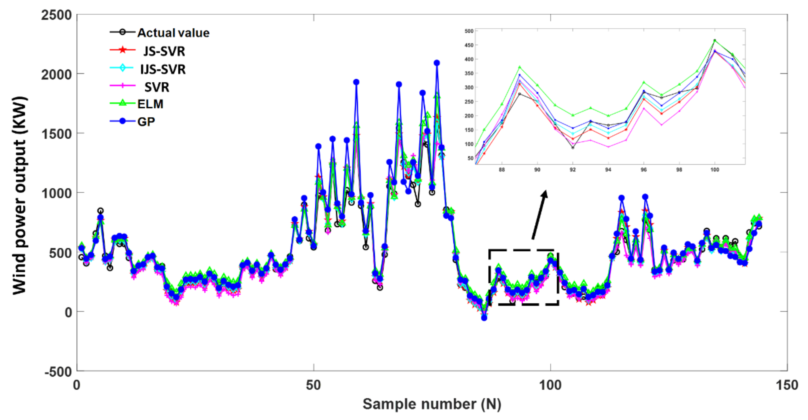
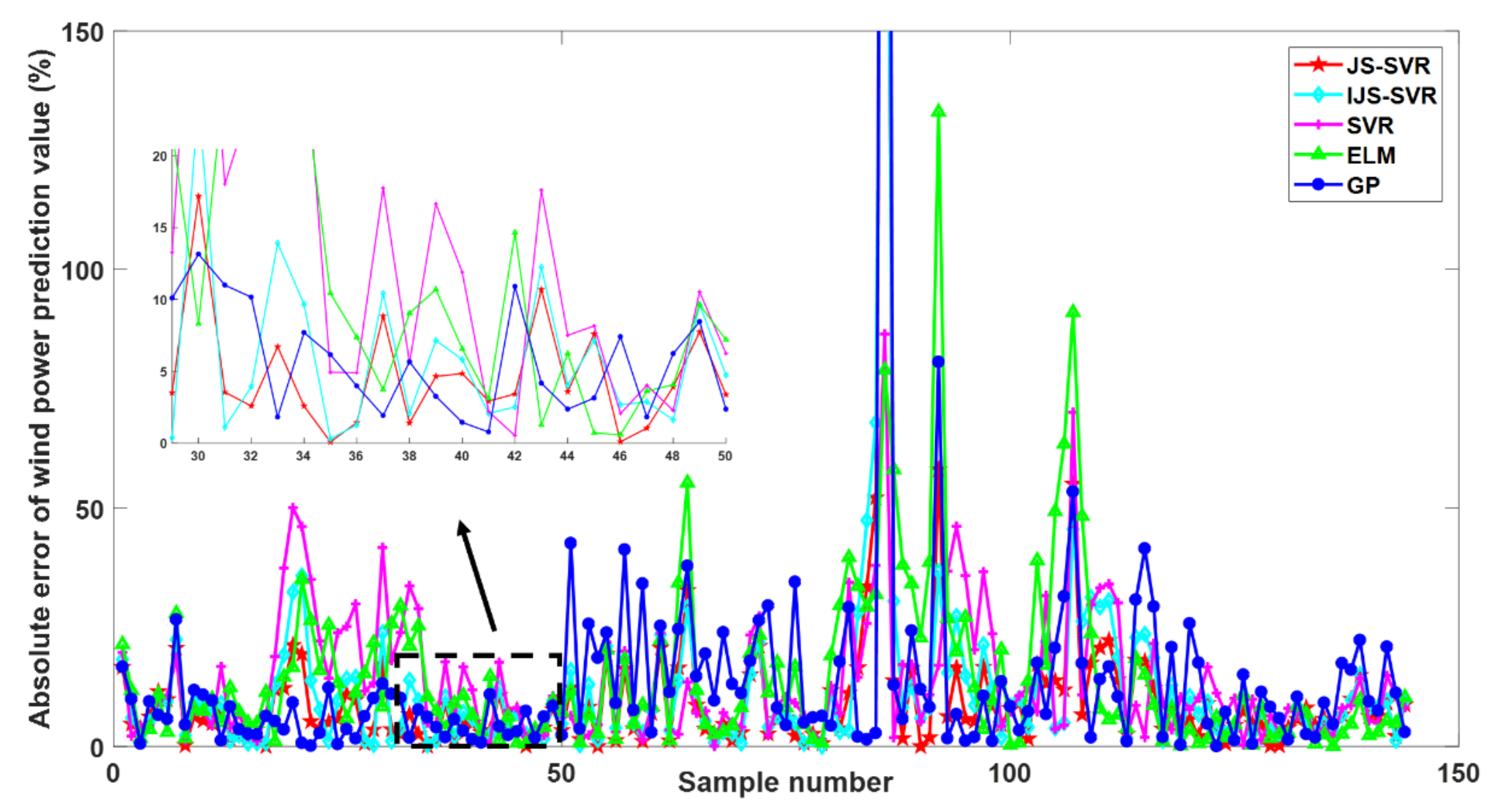
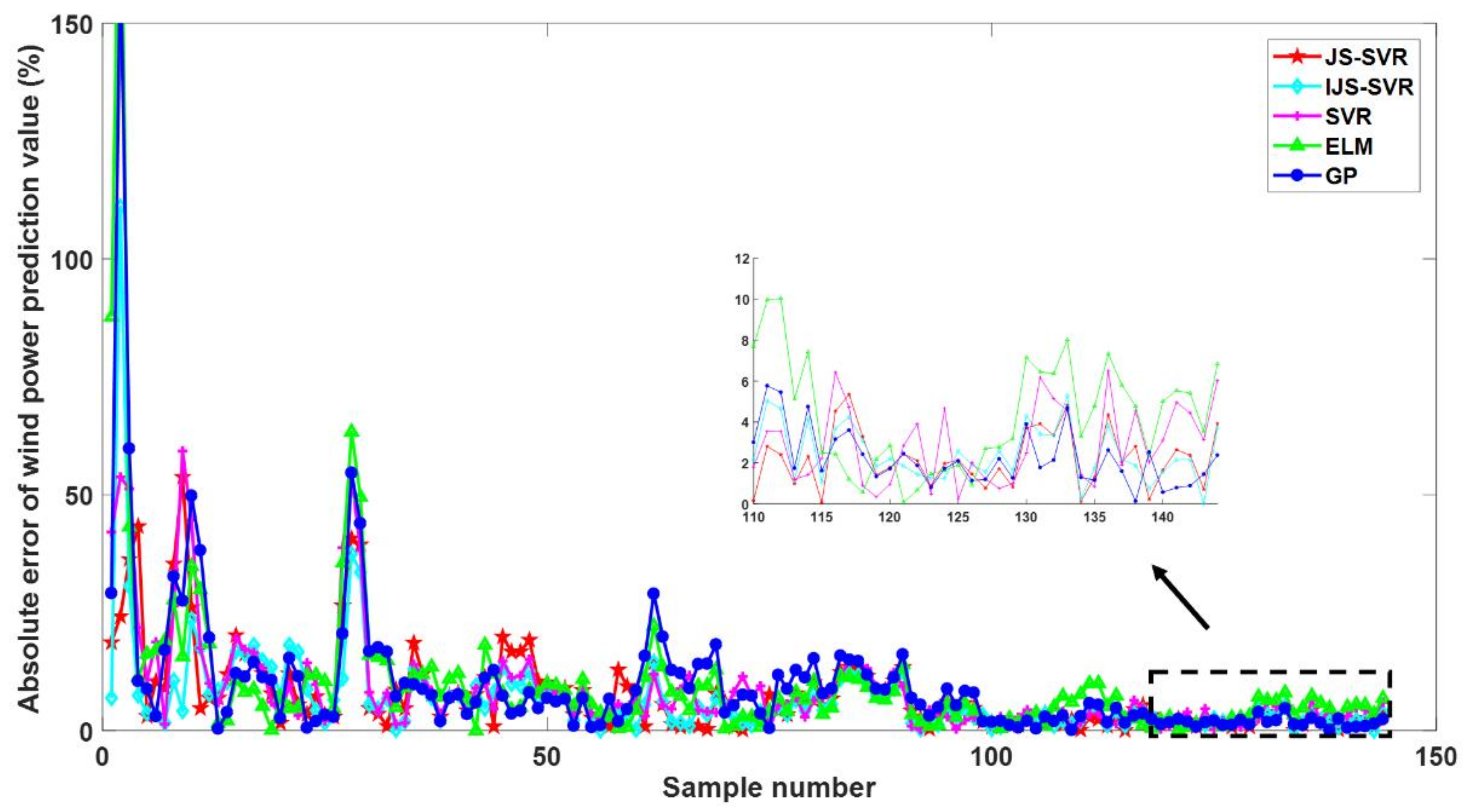
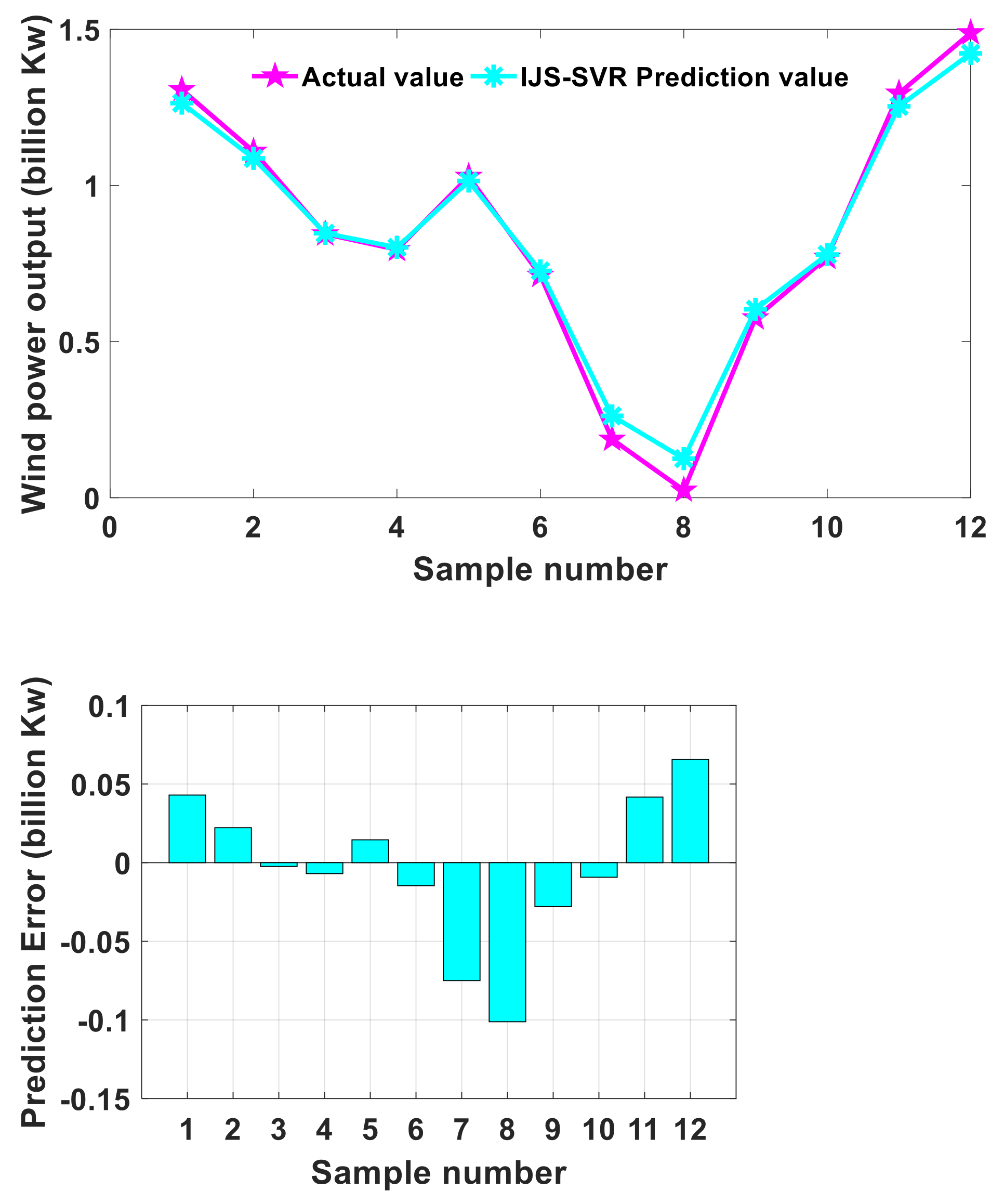
An IJS-SVR model was proposed in this study. Compared with other methods, the IJS-SVR model proposed in this study could achieve better prediction results than other models in both seasons, and its prediction performance was better, which can improve the prediction accuracy of wind power.

(2)

The IJS algorithm was proposed. Compared with the comparative algorithms, the optimized values of IJS were all closer to 0. It exhibited good convergence ability, search stability, and optimization ability, as well as being more suitable for solving optimization problems.

(3)

This study provides a more economical and effective method of wind power to solve its uncertainties, and can be used as a reference for grid power generation planning and power system economic dispatch.

The structure is as follows: the relevant literature review is introduced in Section 2; Section 3 introduces the classical support vector machine model; Section 4 proposes the improved jellyfish algorithm and verifies its effect; the IJS-SVR prediction model is established in Section 5, and its performance is verified; finally, the conclusion and future work are summarized.

2. Literature Review

With the continuous research of scholars at home and abroad, the prediction methods of wind power can be divided into three categories: physical-based methods, statistical-based methods, and hybrid computational intelligence [23] The physical-based methods need to obtain relatively accurate meteorological data, and high prediction accuracy can be obtained with reasonable parameter accuracy. However, this approach requires the construction of complex meteorological acquisition models, and is rarely used in actual situations. Statistical-based methods need to collect a large amount of historical data of power generation, and establish prediction models by analyzing the intrinsic connections between historical data. Traditional statistical methods include Autoregressive Moving Average (ARIMA) and gray prediction model [24,25]. Some advanced machine learning models such as Artificial Neural Networks [26] and Fuzzy System [27], Support Vector Machines, and Bayesian methods [28] have also been applied in wind power forecasting techniques.

Hybrid computational intelligence methods are combinations of artificial intelligence algorithms and computational models. Literature [29] proposed an effective BPNN combined 10 different parameters seeking algorithms and 23 different data sets to accurately predict the power generated in a day, optimizing the prediction accuracy of traditional BPNN, but the model involved more algorithms and was computationally more complex. Literature [30] proposed a BP-based neural network model for hourly PV output prediction. Literature [31] proposed a power forecasting method based on Long Short Term Memory and Back Propagation Neural Network (LSTM-BP), which improved the traditional prediction data set to obtain the average of historical generation data from both horizontal and vertical perspectives, and was trained to obtain higher forecasting accuracy. Literature [32] used Pearson correlation coefficient to select samples similar to the target day as training data and searched for the optimal values of parameters in the limit learning machine by Genetic Algorithm (GA) to construct the SDA-GA-ELM model, and the results showed that the model had high prediction accuracy and high stability. Literature [33] proposed an improved chicken swarm optimization algorithm optimized extreme learning machine (ICSO-ELM) prediction model using an improved chicken flock optimizer to search for optimal values of parameters in the limit learning machine to predict power generation output under various meteorological conditions, and verified the prediction effect of ICSO-ELM by experimental simulation; the results showed that the model had a better prediction effect than the traditional ELM.

Support vector machine (SVM) has advantages in high-dimensional nonlinear prediction models. Literature [34] used extreme random trees to classify daytime weather types into four categories, and based on weather type used multiple machine learning models for power generation prediction, and the results showed that the SVM model outperformed other traditional prediction models when the weather changed frequently. Literature [35] used a SVM model to simplify the complex mathematical problem of output power prediction and combined it with wavelet, radial basis function, and firefly algorithm and verified that the model can obtain more accurate prediction results. Literature [36] proposed a hybrid model combining wavelet transform, particle swarm optimization, and SVM (WT-PSO-SVM), and applied the model to short-term power prediction of real microgrid generation systems. Through experimental comparison, the WT-PSO-SVM model has higher prediction accuracy than SVM. Literature [37] used gray correlation theory for feature selection, and the least squares SVM was optimized used adaptive differential evolution algorithm and evolutionary game theory. The proposed model was used for power generation prediction, and it was verified that the model had a strong generalization capability. Support vector regression (SVR) is the application of SVM in nonlinear prediction. SVR has the advantages of effectively solving the nonlinear regression problem, fast training speed, and strong generalization ability in power prediction.

The SVR was selected as the basic model for wind power prediction in this study [38]. Since the predictive ability of the SVR model is very sensitive to its parameters, an intelligent algorithm, jellyfish search algorithm (JS), to select the optimal parameters can improve the model accuracy. To improve the performance of JS, the Sobol sequence and chaotic mapping initialization method were used to optimize the initial position of the population. A sinusoidal dynamic adaptive factor was introduced into the position update formula to further improve the local search capability of the JS algorithm. The population variation operation was introduced to further enhance the global search capability while enriching the population diversity. An improved jellyfish search algorithm (IJS) was proposed. Therefore, the IJS was used to optimize the parameters of SVR, based on which an IJS-SVR prediction model was proposed to predict wind power aiming to achieve more accurate prediction results and provide guidance for the decision making of wind power farms.

3. Methods

3.1. Support Vector Regression Model

The Support Vector Regression (SVR) model can solve small sample, non-linear, and high dimensional problems. The SVR model can be used to deal with wind power prediction of non-stationary sequence.

Given a data set $\left\{(x_1,y_1),(x_2,y_2),\dots (x_i,y_i)\right\},i\in \left[1,2,\dots ,n\right]$, $x_i$ and $y_i$ are the inputs and outputs. n is the total number of samples. The linear regression equation for constructing the SVR model can be expressed as follows:

$$f\left(x\right)=a^T\cdot x+b$$

(1)

where, a is the weight; and b is the bias constant, which can be obtained by training the SVR model.

The prediction objective of the SVR model is to minimize the error between the predicted $f\left(x\right)$-value and the actual value y, but the problem of weak generalization ability may occur. Therefore, setting the existence of error $\epsilon$ between the true value and predicted value as a reasonable result, the objective function of SVR is as follows:

$$\min \frac{1}{2}{‖a‖}^2+C{\displaystyle {\sum }_{i=1}^m({\xi }_i+{\xi }_i^{*})}$$

(2)

$$s.t.\left\{\begin{array}{l}{y}_i-f(x_i)\le \epsilon +{\xi }_i\\ f(x_i)-y_i\le \epsilon +{\xi }_{{}_i}^{*}\\ {\xi }_i\ge 0,{\xi }_{{}_i}^{*}\ge 0\end{array}\right.$$

(3)

where, C is the penalty factor; ${\xi }_i$ and ${\xi }_i^{*}$ are the slack variables can measure the degree of deviation; $\epsilon$ is the error; and m is the number of training samples.

The nonlinear regression was obtained by solving the pairwise optimization problem, which is expressed as follows:

$$f(x)={\displaystyle {\sum }_{i=1}^m({\alpha }_i^{*}-{\alpha }_i)K(x_i,x)}+b$$

(4)

The selection of the kernel function affects the performance of the SVR model. The Gaussian kernel function was selected for the problem of wind power prediction, and the equation is as follows:

$$K(x_i,x)=\exp (-\frac{{‖x_i-x‖}^2}{2{\sigma }^2})$$

(5)

where, $\sigma$ is the bandwidth of the Gaussian kernel, which can affect the prediction performance of the SVR. Meanwhile, the value of the penalty factor C in SVR can also have an impact on the prediction effect of the model. Therefore, an improved artificial jellyfish search (IJS) algorithm was proposed in this study to optimize the penalty function and kernel function parameters in the support vector machine to improve the accuracy of the prediction results.

3.2. Jellyfish Search Algorithm and Improvement

3.2.1. Jellyfish Search Algorithm

Jellyfish search algorithm (JS) is inspired by the search-feeding behavior and movement patterns of jellyfish in the ocean.

The JS algorithm has three rules, which are as follows:

Rule 1: Jellyfish have two types of movement, namely following the ocean currents and moving within the jellyfish population, and switching between the two types of movement is achieved through a time-controlled mechanism.

Rule 2: Jellyfish have search behavior, and when they search for food in the ocean, they are attracted to locations with more food.

Rule 3: The amount of food searched for by jellyfish depends on the location of the food and the objective function of the response.

According to the above rules, a mathematical model of jellyfish movement and its switching mode was established, including jellyfish following ocean current movement, group movement, and time control mechanisms.

(1)

Following ocean current movement

The direction of motion of the current is defined as $\overrightarrow{trend}$, which represents the average of all vector sums from each individual jellyfish position in the current to the current optimal position (the position with the highest amount of food). The mathematical model of the direction of motion of the current $\overrightarrow{trend}$ is expressed as the following equation:

$$\overrightarrow{trend}=\frac{1}{n_{pop}}{\displaystyle {\sum }_{i=1}^{n_{pop}}{\overrightarrow{trend}}_i}$$

(6)

where, n_pop is the population of jellyfish; i is the serial number of each jellyfish in the population; and $\overrightarrow{tren{d}_i}$ is the vector from the position of the i-th jellyfish to the current optimal position, and defines its equation is as follows:

$$\overrightarrow{tren{d}_i}=X^{*}-e_c{X}_i$$

(7)

where, X* represents the current optimal position; X_i represents the position of the ith jellyfish; and e_c represents the factor that determines the attractiveness of food to jellyfish, and the following equation is obtained by iteration:

$$\overrightarrow{trend}=\frac{1}{n_{pop}}{\displaystyle {\sum }_{i=1}^{n_{pop}}\left(X^{*}-e_c{X}_i\right)}=X^{*}-e_c\frac{1}{n_{pop}}{\displaystyle {\sum }_{i=1}^{n_{pop}}{X}_i}=X^{*}-e_c\mu$$

(8)

where, µ represents the average position of all jellyfish in the population; and DF is defined to represent the difference between the jellyfish currently located at the optimal position and the average position of all jellyfish, and the equation defining the DF is expressed as follows:

$$DF=e_c\mu$$

(9)

Substituting Equation (9) into the optimal position equation yields the following:

$$\overrightarrow{trend}=X^{*}-DF$$

(10)

The distribution of jellyfish in the ocean is shown in Figure 1. Where, $\sigma$ is the standard deviation of the normal distribution; and $\beta$ represents the distribution coefficient, which was set to 3 in the algorithm. The range of $\pm \beta \sigma$ around the mean position $\mu$ contains the probability of all jellyfish positions.

A comparative analysis shows that e_c can be expressed as follows:

$$e_c=\beta \times rand(0,1)$$

(11)

The equation for updating the position of jellyfish following the motion of the current was obtained as the following equation:

$$\begin{array}{cc}\hfill X_i\left(t+1\right)& =X_i\left(t\right)+rand(0,1)\times \overrightarrow{trend}\hfill \\ & =X_i\left(t\right)+rand(0,1)\times \left(X^{*}-\beta \times rand(0,1)\times \mu \right)\hfill \end{array}$$

(12)

where, $X_i\left(t\right)$ is the current position of the jellyfish; and $X_i\left(t+1\right)$ is the position of the jellyfish at the next moment after its position has been updated.

(2)

Group movements

The group movement of jellyfish is divided into passive movement (Class A) and active movement (Class B), with Class A movement mostly occurring when the jellyfish swarm is first formed, and with the passage of time the jellyfish more often carry out Class B movement. Class A movement is manifested as the jellyfish moving around its current position, and its position update equation is as follows:

$$X_i\left(t+1\right)=X_i\left(t\right)+\gamma \times rand(0,1)\times \left(U_b-L_b\right)$$

(13)

where, U_b is the upper bound of the search space; L_b is the lower bound; $\gamma$ is the motion coefficient of the jellyfish, and $\gamma$ is taken as 0.1 in the algorithm. The movement range of the jellyfish depends on the set values of U_b, L_b, and $\gamma$.

Jellyfish performing Class B movement will approach the individual jellyfish with more food at their location and gather with food content as their target, and the equation for updating the position of jellyfish performing Class B movement is expressed as follows:

$$X_i\left(t+1\right)=X_i\left(t\right)+\overrightarrow{step}$$

(14)

where, $\overrightarrow{step}$ represents the step length of jellyfish i with direction of motion, and the equation defines $\overrightarrow{step}$ and is expressed as follows:

$$\overrightarrow{step}=rand\left(0,1\right)\times \overrightarrow{D}$$

(15)

where, $\overrightarrow{D}$ represents the direction of motion of jellyfish i. The formula for determining the direction of motion is expressed as follows:

$$\overrightarrow{D}=\left\{\begin{array}{l}{X}_j\left(t\right)-X_i\left(t\right),iff\left(X_i\left(t\right)\right)\ge f\left(X_j\left(t\right)\right)\\ X_i\left(t\right)-X_j\left(t\right),iff\left(X_j\left(t\right)\right)\ge f\left(X_i\left(t\right)\right)\end{array}\right.$$

(16)

where, $X_i\left(t\right)$ represents the current position of jellyfish i; $X_j\left(t\right)$ represents the current position of jellyfish j; function f is the objective function with respect to X; in this algorithm, $f\left(X_i\left(t\right)\right)$ represents the food content at the current position of jellyfish i; and $f\left(X_j\left(t\right)\right)$ represents the food content at the current position of jellyfish j.

(3)

Time control mechanism

In order to simulate and realize the switching between the three modes of motion of jellyfish, a time control mechanism was set and expressed as a time control function $c\left(t\right)$. The formula defining $c\left(t\right)$ is expressed as follows:

$$c\left(t\right)=\left|\left(1-\frac{t}{T}\right)\times \left(2\times rand\left(0,1\right)-1\right)\right|$$

(17)

where, t is the current iterations; T is the maximum number of iterations; $c\left(t\right)$ is a random number between 0 and 1. $c\left(t\right)\ge 0.5$ was set as the range of values to control the movement of jellyfish following the ocean currents; $c\left(t\right)<0.5$ was set as the range of values to control the intra-group movement of jellyfish.

3.2.2. Improved Jellyfish Search Algorithm

The JS is prone to insufficient local search or global search capability when applied to solve high-dimensional problems. In this section, the Improved Jellyfish Search (IJS) algorithm is proposed, and its detailed description is as follows:

(1)

Improvement of population location initialization strategy

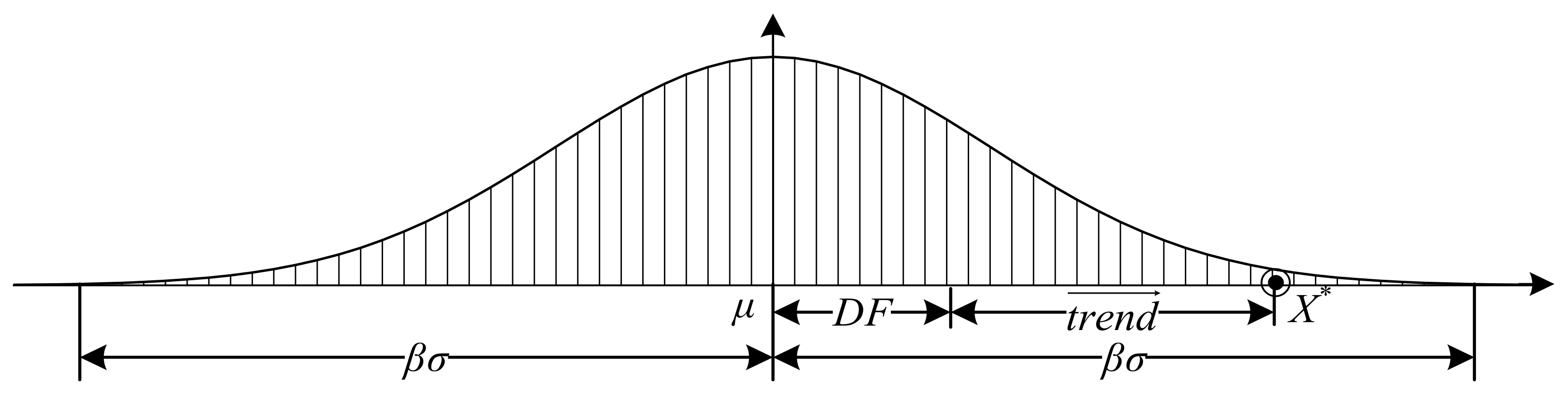
The Sobol sequence and chaotic mapping initialization strategies were used to generate half of the population each. The Sobol sequence can generate the initial position of jellyfish population more uniformly under the condition of satisfying the search range constraint. There are various methods of chaotic mapping, and in this study, we chose Tent mapping, whose functional representation is expressed as follows:

$$x_{t+1}=\left\{\begin{array}{l}{x}_t/\alpha x_t\in \left[0,\alpha \right]\\ \left(1-x_t\right)/\left(1-\alpha \right) x_t\in \left(\alpha ,1\right]\end{array}\right.$$

(18)

where, x_t represents the generated chaotic sequence; $t\in \left[1,2,\dots ,n\right]$; n represents the number of individuals in the jellyfish population to be initialized; $\alpha$ is the adjustment parameter, which takes the value of 0.5.

The population generated by introducing the above method can enrich the population diversity while making the distribution of the population in the solution space more uniform, and can effectively avoid the local optimum situation.

(2)

Sinusoidal dynamic adaptive factor

To improve the local search capability of the artificial jellyfish search algorithm, a sinusoidal adaptive factor was introduced and its expression is defined as follows:

$$S=1+\sin \frac{\pi (2T+t)}{2T}$$

(19)

where, S represents the sinusoidal dynamic adaptive factor; T is the maximum iterations; t is the current iterations.

After introducing the sinusoidal dynamic adaptive factor S, the position update formula for jellyfish performing class A motion can be obtained and expressed as follows:

$$X_i\left(t+1\right)=X_i\left(t\right)+S\times \gamma \times rand(0,1)\times \left(U_b-L_b\right)$$

(20)

The improved position update formula is able to dynamically adjust the search range of jellyfish as the iterations increases so as to improve the algorithm’s search capability overall.

(3)

Population variation operation

The random variation operation was added to the artificial jellyfish search algorithm, aiming to enrich the population diversity while enhancing the global search capability, as follows:

Operation 1: After the jellyfish finish moving according to the position update formula and calculate the fitness value, a jellyfish individual X_k was selected from the current population, and then three jellyfish individuals were randomly selected and the fitness values were sorted from best to worst to obtain X_a, X_b, and X_c, whose fitness values are f_a, f_b, and f_c, respectively, and then a new jellyfish position was calculated based on the positions of the three individuals for updating the current position of X_k, resulting in a variation. The formula for calculating the new position of X_k is expressed as follows:

$$X_k=X_a+\delta \left(X_b-X_c\right)$$

(21)

where, $\delta$ is the variational operator, and its formula is expressed as follows:

$$\delta ={\delta }_l+\left({\delta }_u-{\delta }_l\right)\times \frac{f_b-f_a}{f_c-f_a}$$

(22)

where, ${\delta }_u$ and ${\delta }_l$ are the upper and lower bounds of variability, taken as 0.9 and 0.1, respectively.

Operation 2: The mutant population was cross-swapped with the population before the mutation, by randomly generating R between 0 and 1, and then it was compared with the set random crossover parameter CR, which is expressed by the formula as follows:

$$CR=\frac{1}{2}\times \left(1+rand\left(0,1\right)\right)$$

(23)

If the value of the random number R is greater than CR, the jellyfish individuals in the mutant population corresponding to it were replaced using the jellyfish individuals before the mutation, otherwise the positions of the jellyfish individuals in the mutant population were kept unchanged.

Operation 3: The fitness values of each jellyfish in the population after the mutation and crossover operations were calculated one by one, and then compared with the fitness values of individual jellyfish in the population before the mutation; the better jellyfish in the population after the mutation and crossover were retained, and the corresponding jellyfish in the population before the mutation were replaced, finally completing the population renewal.

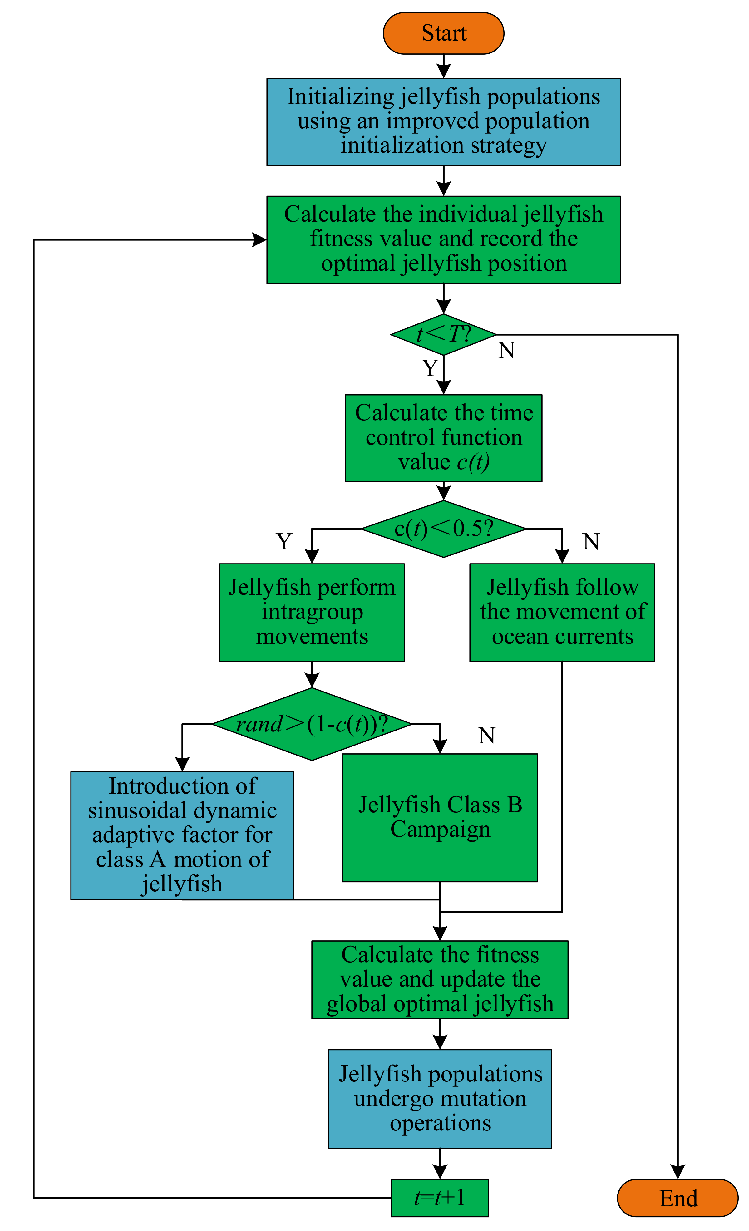
3.2.3. Steps of IJS Algorithm

By introducing the above three improvement methods, the improvement of the artificial jellyfish search algorithm is completed, and thus the improved artificial jellyfish search algorithm (IJS) is proposed. The flow chart of IJS algorithm optimization is shown in Figure 2.

The steps of the IJS for optimization are as follows:

Step 1: Initialization of the location of the jellyfish population by using the Sobol sequence and chaotic mapping initialization method;

Step 2: Calculating the current fitness values corresponding to all jellyfish positions and recording the current positions of jellyfish with optimal fitness values.

Step 3: Start iterative optimization, determine whether the current iterations t is less than the maximum iterations T; if yes, then proceed to step 4; if otherwise, end the iteration.

Step 4: Calculate the time control function c(t), when $c\left(t\right)<0.5$, the jellyfish carry out group movement and update the current position before proceeding to step 5. When $c\left(t\right)\ge 0.5$, follow the current movement and update the current position before proceeding to step 6.

Step 5: The generated random number between 0 and 1 is compared with the value of 1 − c(t), and if the random number is larger, the current position is updated using the class A motion with the introduction of a sinusoidal dynamic adaptive factor; if the random number is less than or equal to 1 − c(t), the current position is updated using the class B motion, both followed by step 6.

Step 6: The adaptation values corresponding to all current jellyfish positions are calculated, and the current positions of jellyfish with optimal adaptation value are recorded.

Step 7: Use the population mutation operation to mutate and cross the positions of the jellyfish population and complete the population update.

Step 8: After increasing the number of iterations once, return to Step 2.

3.3. Test of Algorithm Performance

In this study, the IJS algorithm was tested for its performance. Six benchmark functions in CEC2013 were selected for the performance testing in this study. Three single-peak functions from F1–F3 and three multi-peak functions from F4–F6 were selected, and the details of the benchmark test functions are shown in

Table 1. Benchmark test functions.

Function	Range	opt
$F_1(x)={\displaystyle {\sum }_{i=1}^n{x}_i{}^2}$	[−100, 100]	0
$F_2(x)={\displaystyle {\sum }_{i=1}^n\left|x_i\right|}+{\displaystyle {\prod }_{i=1}^n\left|x_i\right|}$	[−10, 10]	0
$F_3(x)={{\displaystyle {\sum }_{i=1}^n\left({\displaystyle {\sum }_{j-1}^i{x}_j}\right)}}^2$	[−100, 100]	0
$F_4\left(x\right)={\displaystyle {\sum }_{i=1}^n\left[x_i{}^2-10\cos \left(2\pi x_i\right)+10\right]}$	[−5.12, 5.12]	0
$F_5(x)=-20\exp (-0.2\sqrt{\frac{1}{n}{\displaystyle {\sum }_{i=1}^n{x}_i^2}})-\exp (\frac{1}{n}{\displaystyle {\sum }_{i=1}^n\cos (2\pi x_i)})+20+e$	[−32, 32]	0
$F_6(x)=\frac{1}{4000}{\displaystyle {\sum }_{i=1}^n{x}_i^2}-{\displaystyle {\prod }_{i=1}^n\cos (\frac{x_i}{\sqrt{i}})+1}$	[−600, 600]	0

.

It can be seen from Table 1 that the optimal value of the test function within the value range was 0. Additionally, 0 is the optimal convergence result. The closer to 0 that the value that the optimization algorithm can converge to is, the stronger the optimization and convergence ability of the algorithm.

In order to verify the convergence of the IJS algorithm, the traditional JS algorithm, the Particle Swarm Optimization (PSO), Seagull Optimization Algorithm (SOA), Ant-Lion Optimization (ALO), and Grasshopper Optimization Algorithm (GOA) were selected as the comparison algorithms. All algorithms were tested with the above six benchmark test functions in the same test environment. Algorithm parameter settings are shown in

Table 2. Setting of parameters in some algorithms.

Algorithm	Parameters	Value	Max-Iteration	Population	Dimension
JS	Motion coefficient	0.1	500	30	30
GOA	Decreasing factor	max = 1, min = 0.00001	500	30	30
PSO	Inertia factor	max = 0.9, min = 0.4	500	30	30
	Acceleration factor	C1 = C2 = 2	500	30	30
SOA	Control Factors	2	500	30	30
	Spiral shape parameters	u = 1, v = 1	500	30	30

.

To evaluate the performance results more objectively, each algorithm was tested 30 times, and the final convergence values of all algorithms after each test were recorded. The average value (AVE) and the standard deviation (STD) were recorded after 30 iterations as the algorithm evaluation indexes. The test results of the algorithms under single-peak and multi-peak test functions are shown in

Table 3. The results of each algorithm under the single-peak test function.

	F1		F2		F3
Algorithm	AVE	STD	AVE	STD	AVE	STD
JS	7.20 × 10−23	3.94 × 10−22	4.95 × 10−10	2.71 × 10−9	3.33 × 101	1.05 × 102
IJS	7.41 × 10−120	4.06 × 10−119	5.22 × 10−69	2.72 × 10−68	3.96 × 10−6	2.17 × 10−5
SOA	8.42 × 10−12	1.44 × 10−11	1.78 × 10−8	1.41 × 10−8	1.76 × 10−3	8.13 × 10−3
PSO	1.56 × 10−1	9.09 × 10−2	1.62 × 100	6.64 × 10−1	8.41 × 101	3.07 × 101
GOA	2.08 × 10−8	3.17 × 10−8	2.02 × 100	2.82 × 100	7.22 × 10−6	2.37 × 10−5
ALO	1.06 × 101	1.91 × 101	1.22 × 102	8.02 × 101	7.86 × 10−2	2.97 × 10−1

and

Table 4. The results of each algorithm under the multi-peak test function.

	F4		F5		F6
Algorithm	AVE	STD	AVE	STD	AVE	STD
JS	1.70 × 10−1	6.22 × 10−1	6.97 × 10−14	2.16 × 10−13	0	0
IJS	0	0	1.84 × 10−15	1.60 × 10−15	0	0
SOA	2.73 × 100	4.78 × 100	2.00 × 101	1.74 × 10−3	2.09 × 10−2	3.32 × 10−2
PSO	1.54 × 102	2.52 × 101	2.87 × 10−1	5.04 × 10−1	7.66 × 10−3	7.89 × 10−3
GOA	9.83 × 100	6.74 × 100	5.88 × 10−1	8.70 × 10−1	1.61 × 10−1	8.20 × 10−2
ALO	1.61 × 102	2.81 × 101	4.73 × 10−1	6.46 × 10−1	1.76 × 10−1	7.11 × 10−2

.

As can be seen from Table 3 and Table 4, among all the tested functions, the convergence mean of the IJS algorithm was closest to 0 after 30 tests, and the standard deviation of the convergence value was also the smallest among all the algorithms. IJS had the best convergence ability and search stability. For F6, the average value of JS and IJS converged to 0 and the standard deviation was also 0. This indicates that JS and IJS all searched for the theoretical optimal value. Therefore, the IJS algorithm proposed in this study is the algorithm with the best search capability and optimal search stability, which is more suitable for solving optimization problems.

4. Establishment of Prediction Model

4.1. Selection of Objective Function and Evaluation Index

According to the data characteristics and prediction requirements of wind power generation, Mean Square Error (MSE)was selected as the objective function, and its function form is shown:

$$F_{obj}=MSE=\frac{1}{m}{{\displaystyle {\sum }_{i=1}^m\left(y_i-{\widehat{y}}_i\right)}}^2$$

(24)

where, F_obj represents the objective function; m is the quantity of output power data to be predicted; $y_i$ is the real value of the output power; ${\widehat{y}}_i$ is the predicted value of the output power.

In this study, mean absolute error (MAE), mean absolute percentage error (MAPE), fitting coefficient (R²), and root mean square error (RMSE) were selected as the evaluation indexes of the prediction model. The detailed equations are as follows:

$$MAE=\frac{1}{m}{\displaystyle {\sum }_{i=1}^m\left|{\widehat{y}}_i-y_i\right|}$$

(25)

$$MAPE=\frac{1}{m}{\displaystyle {\sum }_{i=1}^m\left|\frac{{\widehat{y}}_i-y_i}{y_i}\right|}\times 100\%$$

(26)

$$R^2=1-\frac{{\displaystyle {\sum }_{i=1}^m{\left(y_i-{\widehat{y}}_i\right)}^2}}{{\displaystyle {\sum }_{i=1}^m{\left(y_i-\overline{y}\right)}^2}}$$

(27)

$$RMSE=\sqrt{\frac{1}{m}{\displaystyle {\sum }_{i=1}^m{\left({\widehat{y}}_i-y_i\right)}^2}}$$

(28)

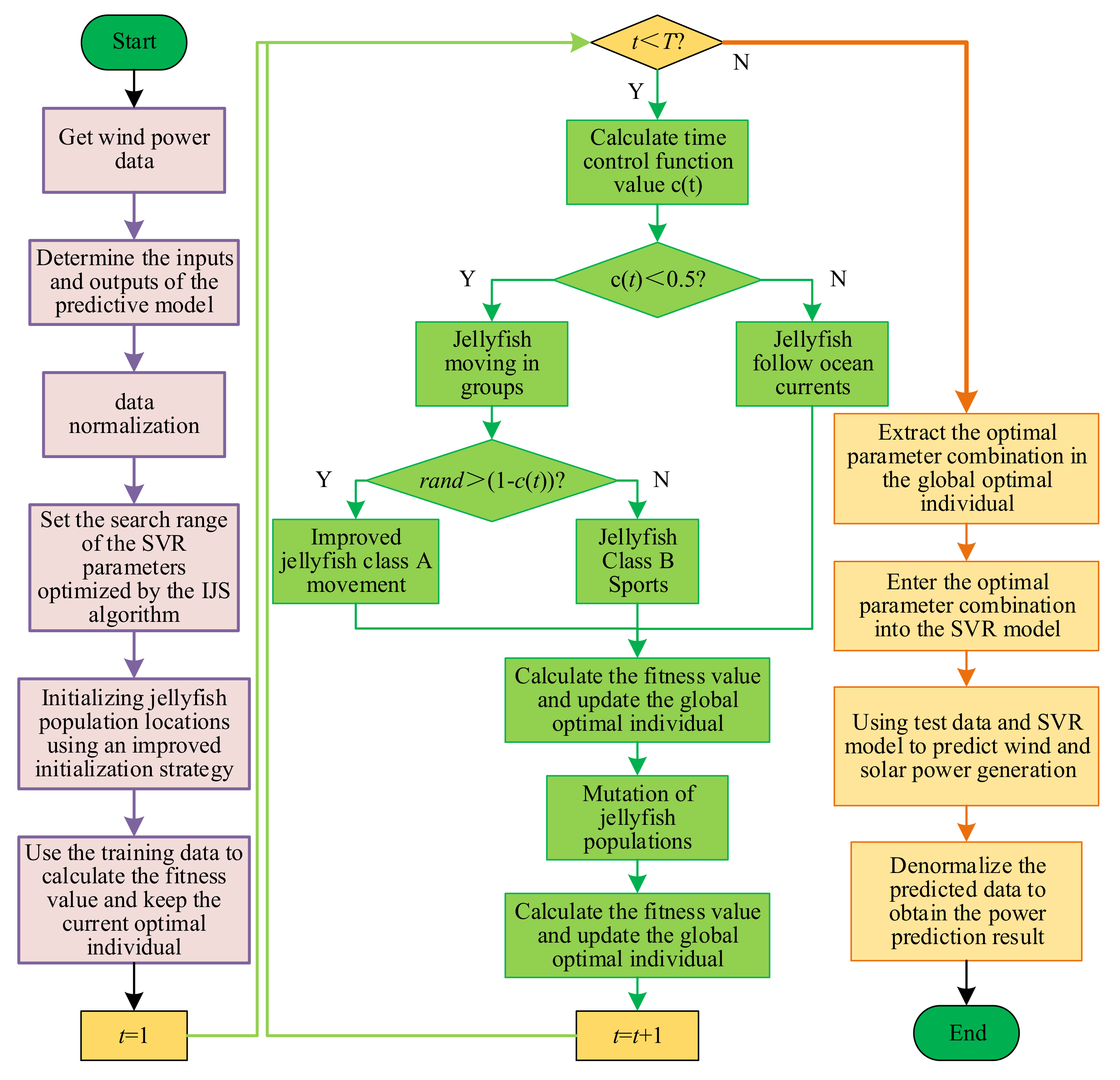
4.2. Establishment of the Wind Power Prediction Model Based on IJS-SVR

The key performance parameters of the SVR model are the penalty coefficient C and the kernel function parameter $\sigma$, which determine the accuracy of the prediction results. In this study, the proposed IJS algorithm was used to optimize the SVR model. A wind power prediction model based on IJS-SVR was established. The specific prediction steps are as follows:

Step 1: The wind power data were classified into training data and test data, in Section 5.1, and the training data and test data were determined;

Step 2: The input and output data of the prediction model are determined; the input data include wind speed and direction, and the output data are the output power;

Step 3: The data are normalization processed;

Step 4: Parameters setting. Set the populations of jellyfish N to 30, the maximum number of iterations T to 500, the dimension D to 2, the search range of C as [0.1, 1200], and the search range of $\sigma$ as [0.01, 100];

Step 5: Use the improved initialization strategy to initialize the jellyfish population;

Step 6: Calculate the fitness value of all individuals in the population, and record the position of the jellyfish individual with the best fitness value;

Step 7: Iterative optimization; select one of the three jellyfish movement modes through the time control mechanism, and use the position update equation corresponding to the selected movement mode to update the jellyfish position;

Step 8: Calculate the fitness value of the individual in each generation and record and update the global optimal jellyfish individual;

Step 9: Perform mutation operation on the jellyfish population, update the position of the jellyfish in the population, calculate the fitness value, and record and update the global optimal individual;

Step 10: If the number of iterations t does not reach the maximum value T, go to Step 7; if the number of iterations reaches the maximum value, the iteration ends, and the global optimal individual is output, continue to Step 11;

Step 11: The globally optimal individual position corresponds to the optimal parameters, the optimal parameters are introduced into the SVR model; based on this, the IJS-SVR model is established;

Step 12: The IJS-SVR model is used to predict wind power by test data;

Step 13: Reverse the predicted result, and obtain the predicted value of wind power.

The flow chart of wind power prediction based on IJS-SVR model is shown in Figure 3.

5. Result Analysis

5.1. Data Source and Processing

The wind power data came from the public data of the La Haute Borne wind farm in France [39]. The farm conducts data sampling every 10 min. The sampling data include wind output power, wind direction, wind speed, ambient temperature, and relative humidity.

Wind power is susceptible to seasonal conditions. In this study, spring and winter were considered in predicting. The data from 4–11 May 2017 were used as research data in spring. The data from 4–10 May 2017 were used as training data, and the data from 11 May 2017 were used as test data. The data from 8–15 December 2017 were used as research data in winter, in which the data from 8–14 December 2017 were used as training data, and the data from 15 December 2017 were used as test data. The above-mentioned daily research data are in the time period from 0:00 to 24:00, and there are 144 data sample points per day.

Due to fact that the output power is inconsistent with the units of meteorological indicators such as wind speed and wind direction, the value ranges are also different. If the data are directly applied to the power prediction, they are prone to large prediction errors. In order to avoid this phenomenon, it is necessary to preprocess the training data and test data, and normalize the data in different units and value ranges. The normalization equation is shown:

$$A_N=\frac{A-A_{\min }}{A_{\max }-A_{\min }}$$

(29)

where, A is the variable value to be normalized, such as output power, ambient temperature, wind speed, and wind direction and so on; A_min is the minimum value of the variable; A_max is the maximum value of the variable; A_N is the variable after normalization. After normalization, the variable values are limited between 0 and 1, which can effectively avoid the problem of large prediction errors caused by inconsistent units and value ranges between different variables.

5.2. Analysis of Prediction Results

5.2.1. Case 1

Case 1 is a prediction study of wind power in spring using each prediction models. JS-SVR, IJS-SVR, SVR, ELM, and GP were used to predict the output power of wind. The actual values of the output power and the predicted values after prediction by each model are shown in Figure 4.

It can be seen from Figure 4 that IJS-SVR, JS-SVR, SVR, ELM, and GP models could realize the prediction of wind power. However, different models had different mining capabilities for wind power data. Compared with the GP and ELM models, the prediction results of the SVR model were closer to the actual value. Therefore, the SVR model could better describe the trend of actual wind power. The evaluation index values of IJS-SVR, JS-SVR, SVR, ELM, and GP prediction models are shown in

Table 5. Evaluation index values of each prediction model in spring.

Model	MAE (KW)	MAPE (%)	R2 (%)	RMSE (KW)	T (s)
JS-SVR	39.48	12.50	97.29	53.95	6.09
IJS-SVR	33.48	10.76	97.94	47.03	6.22
SVR	48.76	13.80	96.24	63.63	0.33
ELM	48.42	14.82	95.85	66.83	1.53
GP	65.36	14.72	87.49	116.0	32.60

. The absolute error value curves of prediction results in spring of each model are shown in Figure 5.

It can be seen from Table 5 that, compared with the GP and ELM models, the MAPE of the SVR model was reduced by 6.874% and 6.246%, respectively. The R2 of SVR model was higher, 0.389% and 8.747%, than that of the GP and ELM models. Under the RMSE, the RMSE of the SVR model was 45.148% and 5.042% lower than that of the GP and ELM models. As can be seen from Figure 5, the absolute error value of the prediction result of the SVR model was closer to 0 than the values of the other two original models. Compared with ELM and GP, the running time of SVR model was shorter. Based on the above analysis, the SVR model has excellent prediction performance, which also confirms the correctness of the selection of the SVR model in this study. Compared with SVR, ELM, and JS-SVR, the running time of the IJS-SVR prediction model was longer and the competitiveness was lower, but IJS-SVR had higher prediction accuracy, and could obtain more accurate wind power output.

In addition, the prediction results of the SVR model after optimization by JS and IJS algorithms were significantly better than the original models of SVR, ELM, and GP. To further verify the validity of the model proposed in this study, the prediction of wind power in winter was further analyzed and studied.

5.2.2. Case 2

Case 2 is a prediction study of wind power in winter by using each prediction model. In winter, JS-SVR, IJS-SVR, SVR, ELM, and GP were used to predict the output power of wind power. The actual value of output power and the predicted value obtained after each prediction model are shown in the Figure 6. The evaluation index values of IJS-SVR, JS-SVR, SVR, ELM, and GP prediction models are shown in

Table 6. Evaluation index values of each prediction model in winter.

Model	MAE (KW)	MAPE (%)	R2 (%)	RMSE (KW)	T (s)
JS-SVR	60.34	7.48	97.75	77.18	10.94
IJS-SVR	53.81	6.75	98.34	66.26	11.66
SVR	65.47	8.56	97.61	79.47	0.35
ELM	72.69	10.18	97.18	86.32	0.27
GP	68.00	9.75	97.44	82.24	32.40

. The absolute error value curves of prediction results in winter of each model are shown in Figure 7.

In Figure 6 and Figure 7, the prediction performance of the IJS-SVR model is significantly better than the other prediction models. The absolute error value of the prediction results of the IJS-SVR model was smaller and more stable. It can be seen from Table 6 that the MAE, MAPE, R2, and RMSE of the JS-SVR model were better than the SVR model. Compared with the SVR, the MAE, MAPE, and RMSE of the JS-SVR model were reduced by 7.827%, 12.64%, and 2.879%, respectively. It is proved that using the JS algorithm to optimize the SVR model can better describe the trend of wind power. It can be seen that the index-R2 of the IJS-SVR model reached more than 98%. This shows that the IJS-SVR model can better fit the wind power data. Compared with the SVR model, the MAE, MAPE, and RMSE of the IJS-SVR model decreased by 17.797%, 21.235%, and 16.617%, respectively, and the R2 increased by 0.728%. Compared with the prediction results of IJS-SVR and the JS-SVR, the IJS-SVR model had better performance and higher prediction accuracy. Therefore, the effectiveness of the IJS algorithm proposed in this study to optimize the SVR model is proven.

5.2.3. Case 3

To better verify the effectiveness and general application of the model proposed in this study, the medium and long-term data of a wind farm were used to verify the performance of IJS-SVR. Months were the data acquisition time node of the wind farm. The four-year wind power output operation data of the wind farm were obtained. The previous three years comprise training data, a total of 36 training sample points. We took the data of the fourth year as the prediction data, with a total of 12 prediction sample points. The medium and long-term prediction results of the IJS-SVR prediction model for the wind farm are shown in Figure 8.

It can be seen from the Figure 8 that the IJS-SVR model proposed in this study can well fit the medium- and long-term data in the wind farm. The R2 of the IJS-SVR model reached as high as 98.80%. Therefore, the IJS-SVR model could be used for medium and long-term prediction.

6. Conclusions

With the continuous expansion of the scale of new energy grid connections, wind power grid connections with randomness and non-stationary characteristics will bring impacts to the power system. Therefore, the high prediction accuracy of wind power has important practical significance for maintaining the safety and stability of the system.

The conclusions are as follows: (1) an improved jellyfish search (IJS) algorithm was proposed for the optimization problem in the wind power prediction. Compared with JS, ALO, GOA, PSO, and SOA, it was proven that IJS has strong optimization ability and can meet the requirements of the optimization problem of wind power prediction. (2) A wind power prediction model based on an improved jellyfish search algorithm optimized by support vector regression was established. JS-SVR, IJS-SVR, SVR, ELM, and GP models were used to predict wind power respectively in spring and winter. According to the analysis of results, compared with other prediction models, the proposed IJS-SVR was closer to the real value. Additionally, the results of the four evaluation indexes were significantly better than other models. (3) It was verified that the IJS-SVR is also suitable for medium- and long-term wind power prediction by using the four-year data of a wind farm and obtained higher prediction accuracy.

The IJS-SVR model proposed in this study still has some limitations: the theoretical output power of the proposed model in this study has a certain deviation from the actual output power. The wide applicability of the IJS-SVR prediction model should be further verified and optimized in the future research.

References

1. Yu, M.; Chen, F.; Zheng, S.; Zhou, J.; Zhao, X.; Wang, Z.; Li, G.; Li, J.; Fan, Y.; Ji, J.; et al. Experimental Investigation of a Novel Solar Micro-Channel Loop-Heat-Pipe Photovoltaic/Thermal (MC-LHP-PV/T) System for Heat and Power Generation. Appl. Energy 2019, 256, 113929. [Google Scholar] [CrossRef]
2. Wang, K.J.; Qi, X.X.; Liu, H.D. A comparison of day-ahead photovoltaic power predicting models based on deep learning neural network. Appl. Energy 2019, 251, 14. [Google Scholar] [CrossRef]
3. Li, L.-L.; Liu, Z.-F.; Tseng, M.-L.; Zheng, S.-J.; Lim, M.K. Improved tunicate swarm algorithm: Solving the dynamic economic emission dispatch problems. Appl. Soft Comput. 2021, 108, 107504. [Google Scholar] [CrossRef]
4. Liu, L.; Zhao, Y.; Chang, D.; Xie, J.; Ma, Z.; Sun, Q.; Yin, H.; Wennersten, R. Prediction of short-term PV power output and uncertainty analysis. Appl. Energy 2018, 228, 700–711. [Google Scholar] [CrossRef]
5. Carvajal-Romo, G.; Valderrama-Mendoza, M.; Rodríguez-Urrego, D.; Rodríguez-Urrego, L. Assessment of solar and wind energy potential in La Guajira, Colombia: Current status, and future prospects. Sustain. Energy Technol. Assess. 2019, 36, 100531. [Google Scholar] [CrossRef]
6. Han, Y.; Wang, N.; Ma, M.; Zhou, H.; Dai, S.; Zhu, H. A PV power interval predicting based on seasonal model and nonparametric estimation algorithm. Sol. Energy 2019, 184, 515–526. [Google Scholar] [CrossRef]
7. Liu, Z.-F.; Li, L.-L.; Liu, Y.-W.; Liu, J.-Q.; Li, H.-Y.; Shen, Q. Dynamic economic emission dispatch considering renewable energy generation: A novel multi-objective optimization approach. Energy 2021, 235, 121407. [Google Scholar] [CrossRef]
8. Niu, T.; Wang, J.Z.; Zhang, K.Q.; Du, P. Multi-step-ahead wind speed predicting based on optimal feature selection and a modified bat algorithm with the cognition strategy. Renew. Energy 2017, 118, 213–229. [Google Scholar] [CrossRef]
9. Monfared, M.; Fazeli, M.; Lewis, R.; Searle, J. Fuzzy Predictor with Additive Learning for Very Short-Term PV Power Generation. IEEE Access 2019, 7, 91183–91192. [Google Scholar] [CrossRef]
10. Liu, H.; Tian, H.Q.; Li, Y.F. Four wind speed multi-step predicting models using extreme learning machines and signal decomposing algorithms. Energy Convers. Manag. 2015, 100, 16–22. [Google Scholar] [CrossRef]
11. Zhou, J.Y.; Shi, J.; Li, G. Fine tuning support vector machines for short-term wind speed predicting. Energy Convers. Manag. 2011, 52, 1990–1998. [Google Scholar] [CrossRef]
12. Wang, K.J.; Qi, X.X.; Liu, H.D.; Song, J.K. Deep belief network based k-means cluster approach for short-term wind power prediction. Energy 2018, 165, 840–852. [Google Scholar] [CrossRef]
13. Wang, H.K.; Song, K.; Cheng, Y. A Hybrid Predicting Model Based on CNN and Informer for Short-Term Wind Power. Front. Energy Res. 2022, 9, 1041. [Google Scholar]
14. Pierro, M.; De Felice, M.; Maggioni, E.; Moser, D.; Perotto, A.; Spada, F.; Cornaro, C. Data-driven upscaling methods for regional photovoltaic power estimation and predict using satellite and numerical weather prediction data. Sol. Energy 2017, 158, 1026–1038. [Google Scholar] [CrossRef]
15. Dai, S.Y.; Niu, D.X.; Han, Y.R. Predicting of Power Grid Investment in China Based on Support Vector Machine Optimized by Differential Evolution Algorithm and Grey Wolf Optimization Algorithm. Appl. Sci. 2018, 8, 636. [Google Scholar] [CrossRef]
16. Yang, L.; He, M.; Zhang, J.S.; Vittal, V. Support-Vector-Machine-Enhanced Markov Model for Short-Term Wind Power Predict. IEEE Trans. Sustain. Energy 2015, 6, 791–799. [Google Scholar] [CrossRef]
17. Cheng, Z.; Liu, Q.; Zhang, W. Improved Probability Prediction Method Research for Photovoltaic Power Output. Appl. Sci. 2019, 9, 2043. [Google Scholar] [CrossRef]
18. Das, U.K.; Tey, K.S.; Seyedmahmoudian, M.; Idna Idris, M.Y.; Mekhilef, S.; Horan, B.; Stojcevski, A. SVR-Based Model to Predict PV Power Generation under Different Weather Conditions. Energies 2017, 10, 17. [Google Scholar] [CrossRef]
19. Li, Y.Q.; Zhou, L.; Gao, P.Q.; Yang, B.; Han, Y.M.; Lian, C. Short-Term Power Generation Predicting of a Photovoltaic Plant Based on PSO-BP and GA-BP Neural Networks. Front. Energy Res. 2021, 9, 8. [Google Scholar]
20. Lin, P.; Peng, Z.; Lai, Y.; Cheng, S.; Chen, Z.; Wu, L. Short-term power prediction for photovoltaic power plants using a hybrid improved Kmeans-GRA-Elman model based on multivariate meteorological factors and historical power datasets. Energy Convers. Manag. 2018, 177, 704–717. [Google Scholar] [CrossRef]
21. Li, J.M.; Ward, J.K.; Tong, J.N.; Collins, L.; Platt, G. Machine learning for solar irradiance predicting of photovoltaic system. Renew. Energy 2015, 90, 542–553. [Google Scholar] [CrossRef]
22. Chou, J.S.; Truong, D.N. A novel metaheuristic optimizer inspired by behavior of jellyfish in ocean. Appl. Math. Comput. 2020, 389, 125535. [Google Scholar] [CrossRef]
23. Das, U.K.; Tey, K.S.; Seyedmahmoudian, M.; Mekhilef, S.; Idris, M.Y.; Van Deventer, W.; Horan, B.; Stojcevski, A. Predicting of photovoltaic power generation and model optimization: A review. Renew. Sustain. Energy Rev. 2017, 81, 912–928. [Google Scholar] [CrossRef]
24. Fara, L.; Diaconu, A.; Craciunescu, D.; Fara, S. Predicting of Energy Production for Photovoltaic Systems Based on ARIMA and ANN Advanced Models. Int. J. Photoenergy 2021, 2021, 6777488. [Google Scholar] [CrossRef]
25. Yu, L.; Ma, X.; Wu, W.; Xiang, X.; Wang, Y.; Zeng, B. Application of a novel time-delayed power-driven grey model to predict photovoltaic power generation in the Asia-Pacific region. Sustain. Energy Technol. Assess. 2020, 44, 14. [Google Scholar]
26. Li, G.; Xie, S.; Wang, B.; Xin, J.; Li, Y.; Du, S. Photovoltaic Power Predicting with a Hybrid Deep Learning Approach. IEEE Access 2020, 8, 175871–175880. [Google Scholar] [CrossRef]
27. Douiri, M.R. Particle swarm optimized neuro-fuzzy system for photovoltaic power predicting model. Sol. Energy 2019, 184, 91–104. [Google Scholar] [CrossRef]
28. Bracale, A.; Caramia, P.; Carpinelli, G.; Di Fazio, A.R.; Ferruzzi, G. A Bayesian Method for Short-Term Probabilistic Forecasting of Photovoltaic Generation in Smart Grid Operation and Control. Energies 2013, 6, 733–747. [Google Scholar] [CrossRef]
29. Al-Dahidi, S.; Ayadi, O.; Adeeb, J.; Louzazni, M. Assessment of Artificial Neural Networks Learning Algorithms and Training Datasets for Solar Photovoltaic Power Production Prediction. Front. Energy Res. 2019, 7, 18. [Google Scholar] [CrossRef]
30. Huang, C.; Cao, L.; Peng, N.; Li, S.; Zhang, J.; Wang, L.; Luo, X.; Wang, J.H. Day-Ahead Predicting of Hourly Photovoltaic Power Based on Robust Multilayer Perception. Sustainability 2018, 10, 8. [Google Scholar] [CrossRef]
31. Hua, C.; Zhu, E.; Kuang, L.; Pi, D. Short-term power prediction of photovoltaic power station based on long short-term memory-back-propagation. Int. J. Distrib. Sens. Netw. 2019, 15, 9. [Google Scholar] [CrossRef]
32. Zhou, Y.; Zhou, N.; Gong, L.; Jiang, M. Prediction of photovoltaic power output based on similar day analysis, genetic algorithm and extreme learning machine. Energy 2020, 204, 10. [Google Scholar] [CrossRef]
33. Liu, Z.-F.; Li, L.-L.; Tseng, M.-L.; Lim, M.K. Prediction short-term photovoltaic power using improved chicken swarm optimizer—Extreme learning machine model. J. Clean. Prod. 2019, 248, 119272. [Google Scholar] [CrossRef]
34. Wang, X.; Sun, Y.; Luo, D.; Peng, J. Comparative study of machine learning approaches for predicting short-term photovoltaic power output based on weather type classification. Energy 2021, 240, 122733. [Google Scholar] [CrossRef]
35. Mojumder, J.C.; Ong, H.C.; Chong, W.T.; Shamshirband, S.; Al Mamoon, A. Application of support vector machine for prediction of electrical and thermal performance in PV/T system. Energy Build. 2016, 111, 267–277. [Google Scholar] [CrossRef]
36. Eseye, A.T.; Zhang, J.H.; Zheng, D.H. Short-term photovoltaic solar power predicting using a hybrid Wavelet-PSO-SVM model based on SCADA and Meteorological information. Renew. Energy 2017, 118, 357–367. [Google Scholar] [CrossRef]
37. Yang, S.X.; Zhu, X.G.; Peng, S.J. Prospect Prediction of Terminal Clean Power Consumption in China via LSSVM Algorithm Based on Improved Evolutionary Game Theory. Energies 2020, 13, 17. [Google Scholar] [CrossRef]
38. Amroune, M.; Bouktir, T.; Musirin, I. Power System Voltage Stability Assessment Using a Hybrid Approach Combining Dragonfly Optimization Algorithm and Support Vector Regression. Arab. J. Sci. Eng. 2018, 43, 3023–3036. [Google Scholar] [CrossRef]
39. Engie. The La Haute Borne Wind Farm. 2018. Available online: https://opendata-renewables.engie.com/explore/?sort=modified (accessed on 21 March 2022).
Figure 1. Distribution of jellyfish in the ocean.
Energies 15 06404 g001
Figure 2. Flow chart of IJS algorithm optimization.
Energies 15 06404 g002
Figure 3. Wind power prediction based on the IJS-SVR model.
Energies 15 06404 g003
Figure 4. The prediction results of each prediction model in spring.
Energies 15 06404 g004
Figure 5. Curve of absolute error values of each prediction model in spring.
Energies 15 06404 g005
Figure 6. Prediction results of each prediction model in winter.
Energies 15 06404 g006
Figure 7. Curve of absolute error values of each prediction model in winter.
Energies 15 06404 g007
Figure 8. The prediction results and error of the IJS-SVR prediction model for the wind farm.
Energies 15 06404 g008