The Non-Stationary Heat Transport inside a Shafted Screw Conveyor Filled with Homogeneous Biomass Heated Electrically

Abstract

The non-stationary heat transfer inside a cylindrical channel of a shafted screw conveyor, electrically heated, and filled with a moving biomass was analyzed. The problem of non-stationary heat transport is encountered in the processes of biomass pyrolysis and food products’ sterilization. To solve the heat conduction equation with initial and boundary conditions, the methods of the expansion of the given and unknown functions into a Fourier series in the angular coordinate, and Fourier and Laplace integral transforms in the axial coordinate and time, respectively, were used. As a result of solving this problem, it is shown that the temperature in the reactor consists of two main terms. The first of them is proportional to time, and the second is a superposition of quasi-monochromatic heat pulses decaying with time. Numerical analysis of the temperature distribution in space and time depending on various specific parameters of the system was carried out. The obtained numerical results were compared with those corresponding to the cases of heat sources in the form of a spiral or a shaftless helical screw.

1. Introduction

Different reactor configurations have been studied for the thermochemical conversion of biomass waste via torrefaction or pyrolysis, e.g., circulating fluidized beds, bubbling fluidized beds, and auger reactors are among the commonly used reactors. The variety of different reactors was reviewed recently [1]. However, the use of auger reactors attracts more and more attention with respect to slow and intermediate pyrolysis or food sterilization. In a fundamental review [2], descriptions of modern screw pyrolysis installations are given, and the advantages and disadvantages of screw reactors are demonstrated. As a rule, the screw reactor is of the shell type. A spiral screw rotating around its axis of symmetry is located inside the fixed shell. The screws can be shaftless or mounted on a central shaft. In industrial applications, the geometry of the screw plays an important role. Depending on the functional needs—conveying, feeding, mixing or their combination—and the process requirements, this geometry is different [3,4,5,6,7,8]. As pyrolysis is an endothermic process it requires a supply of heat. This supply of thermal energy can occur from the wall of the outer surface—the outer shell of the reactor—either through an electrically heated screw, or, as it was often until recently, by direct heating with the help of heat carriers. The passage of electric current through the conductor (screw) generates heat, which occurs as a result of the Joule effect (also known as Ohmic heating or resistive heating). Therefore, it is important when designing the apparatus to obtain the appropriate temperature field inside the reactor, which would contribute to the efficient performance of the pyrolysis process [9] or the sterilization of the food ingredients [10]. As it was demonstrated experimentally by Ledakowicz et al. [11], during the pyrolysis of sewage sludge in an auger reactor with an electrically heated screw, for which the principle of operation was described by Lepez and Sajet in their patent [12], the pyrolysis temperature has a great influence on the product yields and product. Apart from experimental research, mathematical modeling of processes in pyrolysis reactors plays an important role because it is difficult to predict the temperature’s effect on the material used, especially during start-up, considering the transient temperature profile. Shi et al. [13,14] simulated the processes of the slow pyrolysis of biomass in a screw reactor using computational fluid dynamics (CFD) methods, presenting, inter alia, an experimentally determined axial temperature distribution on the screw edge. Nachenius et al. [15] also demonstrated experimental data on temperature changes over time at individual points of the channel, heated by the outer wall of the reactor and not from the screw surface.

At the same time, the problem of the analytical investigation of the temperature distribution in the conveyor while considering all the geometric, mechanical, and thermodynamic parameters of the system remains open. It is a fundamental point of solving the general problem of modeling the chemical reaction of pyrolysis. In earlier papers, we performed a mathematical study of the temperature field inside a reactor with a moving biomass, which was formed due to the resistance heating of the rotating helix [16] and the shaftless helical screw [17].

In this paper, an attempt is made to perform a mathematical modeling of the temperature field in a circular cylindrical reactor, with a thermally insulated surface, filled with a mobile medium, e.g., a biomass, provided that the primary heat is transferred in the reactor from the screw mounted on a rotating insulated shaft, wherein the heat is generated by an electric current due to the Joule–Lenz effect. As in previous works, we will analyze the spatial-temporal changes of the temperature field inside the screw reactor depending on the geometric, kinematic, thermoelectric, and thermodynamic parameters of the screw and the substance filling the channel. Moreover, we also will try to compare the obtained temperature profiles and their temporal changes to the results of previous considerations in simplified models of a single rotating helix and the temperature field generated by an electrically heated shaftless screw conveyor. However, the boundary-initial value problem, which will be next depicted in detail, required a completely different method of solving.

2. Statement of the Boundary-Initial Value Problem of Determining the Temperature Distribution

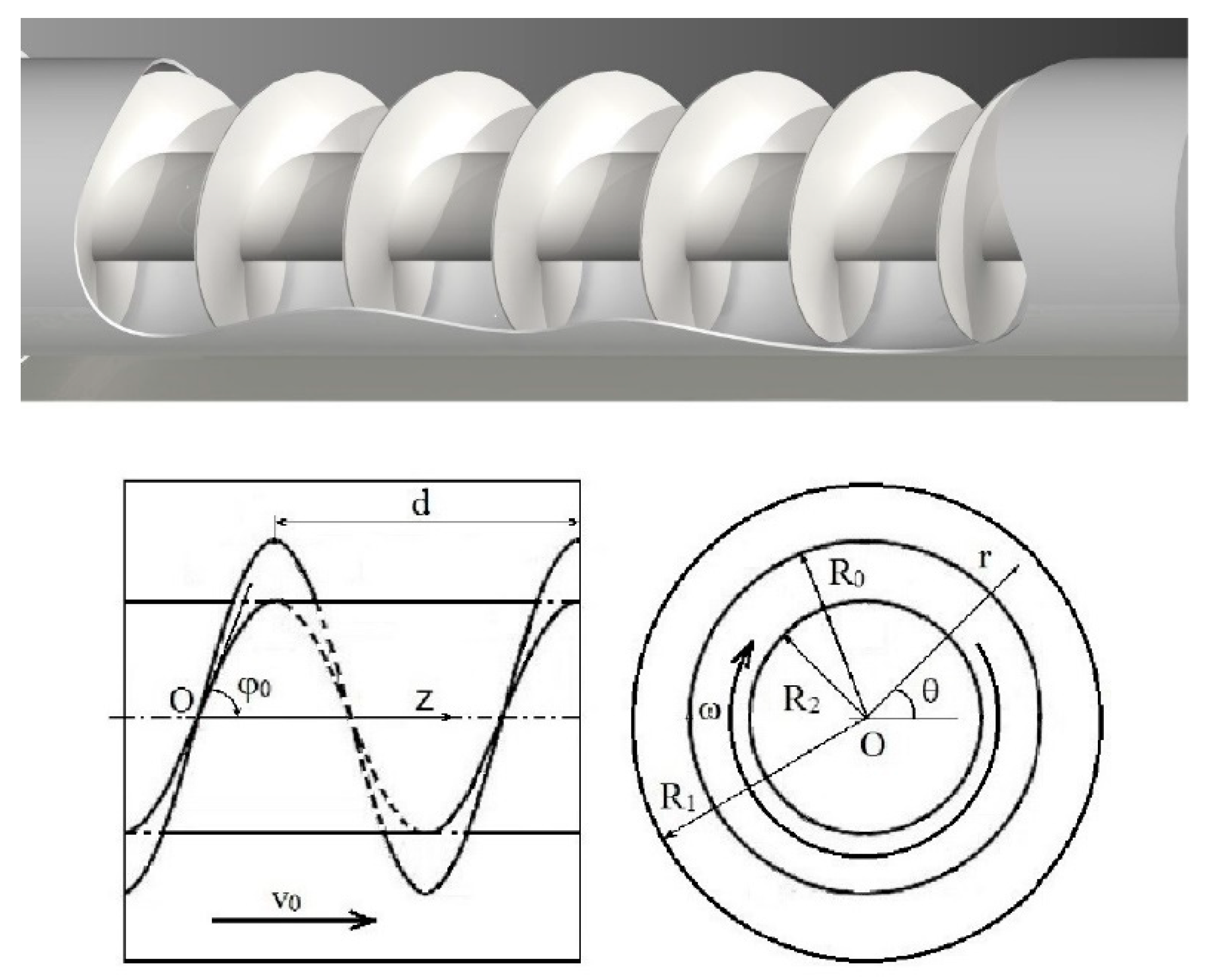
Let us consider a thermally insulated circular cylindrical shell of infinite length and radius R₁. This shell is filled with a homogeneous biomass and contains an auger mounted on a central shaft of radius R₂ (R₁ > R₂). The heat flux on the surface of the shaft is also equal to zero (Figure 1). Suppose that due to the rotation of the screw with angular speed ω, the biomass moves with a constant speed v₀ along the pipe. The source of heat in the channel is the screw shell, as it is heated by electric current I due to the Joule–Lenz thermoelectric effect. The question arises: what will be the distribution of the temperature field in the different parts of the reactor at arbitrary moments in time? This is important because temperature is the main driver of sterilization or pyrolysis processes and their optimal control.

We focus mainly on the problem of the formation of the temperature field by a source with a complex shape, in this case a rotating screw, and pay less attention to the effect of temperature on the movement of biomass. Only the linear movement of the biomass in the axial direction is considered. Otherwise, taking into account the non-linear dependence of the drying processes and chemical reactions in the pyrolysis process on the temperature, it would be impossible to analytically solve this problem of thermal conductivity.

In order to determine the distribution of the temperature inside the material filling the annular reactor channel with the auger, the equation of non-stationary thermal conductivity [18,19] must be solved:

$$\begin{array}{l}{c}_p\rho \left(\frac{\partial T}{\partial \tau }+v_0\frac{\partial T}{\partial z}\right)=\lambda \left[\frac{1}{r}\frac{\partial }{\partial r}\left(r\frac{\partial T}{\partial r}\right)+\frac{1}{r^2}\frac{{\partial }^{2}T}{\partial {\theta }^2}+\frac{{\partial }^{2}T}{\partial z^2}\right]+q\hspace{0.17em}\left(r,\theta ,z,\tau \right),\\ \left(R_2<r<R_1,0<\theta <2\pi ,-\infty <z<\infty ,\tau >0\right)\end{array}$$

(1)

under the initial condition

$${\left.T\right|}_{\tau =0}=T_0$$

(2)

and the boundary conditions of absence of heat flow on the surface of the reactor shell

$${\left.\frac{\partial T}{\partial r}\right|}_{r=R_1}=0$$

(3)

and on the surface of the screw shaft

$${\left.\frac{\partial T}{\partial r}\right|}_{r=R_2}=0,$$

(4)

where ρ is the density of the moving biomass; c_p is its heat capacity at constant pressure; λ is the coefficient of thermal conductivity; r, θ, and z are the cylindrical coordinates with its origin on the axis of the circular channel; and τ is the time.

Assume that there are continuously distributed point sources of heat of the same intensity on the surface of a thin-walled screw. Then, the function q(r, θ, z, τ) describing the total action of these sources will have the form

$$\begin{array}{l}q\left(r,\theta ,z,\tau \right)=\frac{q_0\epsilon r}{\left(\epsilon -{\epsilon }_0\right)R_1^2}\left[H\left(r-R_2\right)-H\left(r-R_0\right)\right]\\ \times {\displaystyle \sum _{m=-\infty }^{\infty }\delta \left[\left(\theta +2\pi m+\omega \tau \right)r\cos {\phi }_0-z\sin {\phi }_0\right]}H\left(\tau \right),\end{array}$$

(5)

where H(x) is the Heaviside step function; δ(x) is the Dirac function; $q_0={\rho }_0{j}^2{R}_1^2$, ρ₀ is the specific electrical resistance of the conductor, j = I/S is the electric current density of a conductor, I = const., S = h × h₁ is the cross-sectional area of the screw, h is its thickness and h₁ = R₀–R₂ is its width, R₀ is the outer radius of the screw, 0 < R₂ < R₀ < R₁, 0 < R₂ < R₀ < R_1, ε = R₀/R₁, ε₀ = R₂/R₁, and φ₀ is the angle of the rise of the screw edge to the axis of the channel Oz (Figure 1; here, the upper figure is for the fragment of the auger, and the lower figures are for the axial and radial sections of the system).

Let us use the following substitution:

$$T\left(r,\theta ,z,\tau \right)-T_0=U\left(r,\theta ,z,\tau \right){\mathrm{e}}^{bz}$$

(6)

then, if b = v₀/(2a), where a is the coefficient of thermal diffusivity of the biomass, a = λ/(c_pρ), the Equation (1) will be given in the form

$$\begin{array}{l}\frac{1}{a}\frac{\partial U}{\partial \tau }-\left[\frac{1}{r}\frac{\partial }{\partial r}\left(r\frac{\partial U}{\partial r}\right)+\frac{1}{r^2}\frac{{\partial }^{2}U}{\partial {\theta }^2}+\frac{{\partial }^{2}U}{\partial z^2}-b^{2}U\right]=Q\left(r,\theta ,z,\tau \right)\\ \left(R_2<r<R_1,0<\theta <2\pi ,-\infty <z<\infty ,\tau >0\right),\end{array}$$

(7)

with appropriate initial and boundary conditions

$${\left.U\right|}_{\tau =0}=0$$

(8)

$${\left.\frac{\partial U}{\partial r}\right|}_{r=R_1}=0$$

(9)

$${\left.\frac{\partial U}{\partial r}\right|}_{r=R_2}=0.$$

(10)

Here

$$Q\left(r,\theta ,z,\tau \right)=\frac{1}{\lambda }{\mathrm{e}}^{-bz}q\left(r,\theta ,z,\tau \right).$$

(11)

3. Analytical Method for Determining the Exact Solution of the Problem

We represent the function U(r, θ, z, τ) as an exponential Fourier series with respect to the angular variable θ [20]

$$U\left(r,\theta ,z,\tau \right)={\displaystyle \sum _{m=-\infty }^{\infty }{U}_m\left(r,z,\tau \right){\mathrm{e}}^{-im\theta }}\left(0<\theta <2\pi \right),$$

(12)

A function q(r, θ, z, τ) can be written in a similar form if using the following property [21]:

$$2\pi {\displaystyle \sum _{m=-\infty }^{\infty }\delta \left(x-2\pi m\right)}={\displaystyle \sum _{m=-\infty }^{\infty }{\mathrm{e}}^{imx}}.$$

(13)

Then, based on Formulas (5) and (11), we obtain

$$Q\left(r,\theta ,z,\tau \right)={\displaystyle \sum _{m=-\infty }^{\infty }{Q}_m\left(r,z,\tau \right){\mathrm{e}}^{-im\theta }}\left(0<\theta <2\pi \right),$$

(14)

where

$$\begin{array}{l}{Q}_m\left(r,z,\tau \right)=\frac{q_0\epsilon {\mathrm{e}}^{-bz}}{2\pi \lambda \left(\epsilon -{\epsilon }_0\right)R_1^2\cos {\phi }_0}\left[H\left(r-R_2\right)-H\left(r-R_0\right)\right]\\ \times \exp \left[-im\left(\omega \tau -\frac{z}{r}\tan {\phi }_0\right)\right]H\left(\tau \right).\end{array}$$

(15)

We also apply to the differential Equation (7) and boundary conditions (9) and (10) the integral Fourier transform over the spatial variable z and the integral Laplace transform over time τ [20]. As a result, taking into account the initial condition (8), we reduce the problem to the ordinary differential equation for the coefficients of expansions into the Fourier series U_m(r, z, τ)

$$\left[\frac{d^2}{d{r}^2}+\frac{1}{r}\frac{d}{dr}-\left(\frac{m^2}{r^2}+s^2\right)\right]U_m^{FL}\left(r,k,p\right)+Q_m^{FL}\left(r,k,p\right)=0\left(R_2<r<R_1\right)$$

(16)

with boundary conditions

$${\left.\frac{d{U}_m^{FL}}{dr}\right|}_{r=R_1}=0,$$

(17)

$${\left.\frac{d{U}_m^{FL}}{dr}\right|}_{r=R_2}=0,$$

(18)

where

$$\begin{array}{l}{U}_m^{FL}\left(r,k,p\right)={\displaystyle \underset{-\infty }{\overset{\infty }{\int }}{\mathrm{e}}^{-ikz}dz}{\displaystyle \underset{0}{\overset{\infty }{\int }}{U}_m\left(r,z,\tau \right){\mathrm{e}}^{-p\tau }d\tau },\\ Q_m^{FL}\left(r,k,p\right)={\displaystyle \underset{-\infty }{\overset{\infty }{\int }}{\mathrm{e}}^{-ikz}dz}{\displaystyle \underset{0}{\overset{\infty }{\int }}{Q}_m\left(r,z,\tau \right){\mathrm{e}}^{-p\tau }d\tau }\left(-\infty <k<\infty ,\mathrm{Re}p>0\right)\end{array}$$

(19)

are Fourier and Laplace transforms of functions U_m(r, z, τ) i Q_m(r, z, τ), and also

$$s=\sqrt{k^2+b^2+p/a}\left(\mathrm{Im}s\ge 0\right).$$

(20)

The solution of the boundary value problems (16)–(18) is obtained in the form of [20]

$$\begin{array}{l}{U}_m^{FL}\left(r,k,p\right)={\displaystyle \underset{0}{\overset{r}{\int }}{D}_m^{FL}\left(r,r^{\prime },k,p\right)Q_m^{FL}\left(r^{\prime },k,p\right)r^{\prime }d{r}^{\prime }}\\ +{\displaystyle \underset{r}{\overset{R_1}{\int }}{D}_m^{FL}\left(r,r^{\prime },k,p\right)Q_m^{FL}\left(r^{\prime },k,p\right)r^{\prime }d{r}^{\prime }}\left(R_2<r<R_1\right),\end{array}$$

(21)

where

$$D_m^{FL}\left(r,r^{\prime },k,p\right)=-\frac{S_m\left(s{R}_1,sr\right)S_m\left(s{R}_2,sr\right)}{{I^{\prime }}_m\left(s{R}_1\right){K^{\prime }}_m\left(s{R}_2\right)-{K^{\prime }}_m\left(s{R}_1\right){I^{\prime }}_m\left(s{R}_2\right)},$$

(22)

$$S_m\left(sx,sy\right)={I^{\prime }}_m\left(sx\right)K_m\left(sy\right)-{K^{\prime }}_m\left(sx\right)I_m\left(sy\right).$$

(23)

Here, I_m(x) is the modified Bessel function of the m-th order, K_m(x) is the McDonald function of the m-th order; the prime symbol denotes the derivatives of these functions.

Applying the inverse integral Fourier and Laplace transforms to Equation (21), after some calculations, we obtain the following result in the form of convolution integrals

$$\begin{array}{l}{U}_m\left(r,z,\tau \right)={\displaystyle \underset{R_2}{\overset{r}{\int }}{r}^{\prime }d{r}^{\prime }{\displaystyle \underset{-\infty }{\overset{\infty }{\int }}d{z}^{\prime }{\displaystyle \underset{0}{\overset{\tau }{\int }}{D}_m\left(r,r^{\prime },z^{\prime },{\tau }^{\prime }\right)Q_m\left(r^{\prime },z-z^{\prime },\tau -{\tau }^{\prime }\right)d{\tau }^{\prime }}}}\\ +{\displaystyle \underset{r}{\overset{R_1}{\int }}{r}^{\prime }d{r}^{\prime }{\displaystyle \underset{-\infty }{\overset{\infty }{\int }}d{z}^{\prime }{\displaystyle \underset{0}{\overset{\tau }{\int }}{D}_m\left(r^{\prime },r,z^{\prime },{\tau }^{\prime }\right)Q_m\left(r^{\prime },z-z^{\prime },\tau -{\tau }^{\prime }\right)d{\tau }^{\prime }}}}\left(R_2<r<R_1\right).\end{array}$$

(24)

Analysis of the asymptotic behavior of this function $D_m^{FL}\left(r,r^{\prime },k,p\right)$ for small arguments sx and sy [22] shows that at m = 0 this function has a singularity s² = 0, i.e., a pole

$$p\equiv p_0=-a\left(k^2+b^2\right).$$

(25)

Instead, for m ≠ 0 singularities s = s_mn= −iμ_mn/R₁ (n = 1, 2, …) of the function $D_m^{FL}\left(r,r^{\prime },k,p\right)$ are zeros of the function

$$g_m\left(s\right)={I^{\prime }}_m\left(s{R}_1\right){K^{\prime }}_m\left(s{R}_2\right)-{K^{\prime }}_m\left(s{R}_1\right){I^{\prime }}_m\left(s{R}_2\right),$$

(26)

which gives, on the basis of Equation (20), the poles

$$p\equiv p_{mn}=-a\left[k^2+b^2+{\left(\frac{{\mu }_{mn}}{R_1}\right)}^2\right]\left(m=0,\pm 1,\pm 2,\mathrm{...};n=1,2,...\right).$$

(27)

There is a relationship between cylindrical functions [22]

$$\begin{array}{l}{I}_m\left(-ix\right)={\mathrm{e}}^{-i\pi m/2}{J}_m\left(x\right),{I^{\prime }}_m\left(-ix\right)=i{\mathrm{e}}^{-i\pi m/2}{J^{\prime }}_m\left(x\right),\\ K_m\left(-ix\right)=\frac{\pi i}{2}{\mathrm{e}}^{i\pi m/2}{H}_m^{\left(1\right)}\left(x\right),{K^{\prime }}_m\left(-ix\right)=-\frac{\pi }{2}{\mathrm{e}}^{i\pi m/2}{H}_m^{\left(1\right)}{}^{\prime }\left(x\right),\end{array}$$

(28)

where J_m(x) is the Bessel function of the m-th order and $H_m^{\left(1\right)}\left(x\right)$ is the Hankel function of the first kind of the m-th order. Therefore, on the basis of Equation (26), we conclude that the characteristic numbers μ_mn will be zeros of the function

$$f_m\left(\mu \right)={J^{\prime }}_m\left(\mu \right){N^{\prime }}_m\left(\mu {\epsilon }_0\right)-{N^{\prime }}_m\left(\mu \right){J^{\prime }}_m\left(\mu {\epsilon }_0\right).$$

(29)

Here, it is taken into account that $H_m^{\left(1\right)}\left(x\right)=\frac{1}{2}\left[J_m\left(x\right)+i{N}_m\left(x\right)\right]$, where N_m(x) is the Neumann function of the m-th order.

Then, after some transformations, from (22) we obtain

$$\begin{array}{l}{D}_m\left(r,r^{\prime },z,\tau \right)=\frac{1}{R_1^2}\sqrt{\frac{a}{\pi \tau }}\exp \left[-\left(a{b}^2\tau +\frac{z^2}{4a\tau }\right)\right]\\ \times \left[\frac{{\delta }_{m0}}{1-{\epsilon }_0^2}+{\left(\frac{\pi }{2}\right)}^2{\displaystyle \sum _{n=1}^{\infty }{A}_{mn}{B}_{mn}\left(\frac{r}{R_1}\right)B_{mn}\left(\frac{r^{\prime }}{R_1}\right)\exp \left(-{\mu }_{mn}^2\frac{a\tau }{R_1^2}\right)}\right]\left(\tau >0\right),\end{array}$$

(30)

where δ_m0 is the Kronecker symbol (δ₀₀ = 1; δ_m0 = 0, m ≠ 0), and

$$A_{mn}=\frac{{\mu }_{mn}^2}{1-{\left(\frac{m}{{\mu }_{mn}}\right)}^2-\left[1-{\left(\frac{m}{{\mu }_{mn}{\epsilon }_0}\right)}^2\right]{\left(\frac{{J^{\prime }}_m\left({\mu }_{mn}\right)}{{J^{\prime }}_m\left({\mu }_{mn}{\epsilon }_0\right)}\right)}^2},$$

(31)

$$B_{mn}\left(r/R_1\right)={J^{\prime }}_m\left({\mu }_{mn}\right)N_m\left({\mu }_{mn}r/R_1\right)-{N^{\prime }}_m\left({\mu }_{mn}\right)J_m\left({\mu }_{mn}r/R_1\right).$$

(32)

It can be shown that due to the symmetry of the function D_m(r, r’, z, τ) with respect to r and r’, the integrants in Equation (24) are equal to each other; therefore, the integrals over r’ in Equation (24) merge into one integral

$$U_m\left(r,z,\tau \right)={\displaystyle \underset{R_2}{\overset{R_1}{\int }}{r}^{\prime }d{r}^{\prime }{\displaystyle \underset{-\infty }{\overset{\infty }{\int }}d{z}^{\prime }{\displaystyle \underset{0}{\overset{\tau }{\int }}{D}_m\left(r,r^{\prime },z^{\prime },{\tau }^{\prime }\right)Q_m\left(r^{\prime },z-z^{\prime },\tau -{\tau }^{\prime }\right)d{\tau }^{\prime }}}}\left(R_2<r<R_1\right).$$

(33)

By substituting in this formula the function Q_m(r, z, τ) from (15), taking into account Equation (30), the integral [23]

$${\displaystyle \underset{-\infty }{\overset{\infty }{\int }}\exp \left[\left(b-\frac{im}{R_0}\tan {\phi }_0\right)z^{\prime }\right]\exp \left(-\frac{{z^{\prime }}^2}{4a{\tau }^{\prime }}\right)d{z}^{\prime }}=2\sqrt{\pi a{\tau }^{\prime }}\exp \left[\left(b-\frac{im}{R_0}\tan {\phi }_0\right)a{\tau }^{\prime }\right]$$

(34)

and the properties of the Dirac function [20]

$${\displaystyle \underset{R_2}{\overset{R_1}{\int }}f\left(r^{\prime }\right)\delta \left(r^{\prime }-R_0\right)d{z}^{\prime }}=f\left(R_0\right)\left(R_2<R_0<R_1\right),$$

(35)

we obtain

$$\begin{array}{l}{U}_m\left(r,z,\tau \right)=\frac{q_0\epsilon {\mathrm{e}}^{-bz}}{\pi \lambda \left(\epsilon -{\epsilon }_0\right)\cos {\phi }_0}\left\{\frac{{\epsilon }^2-{\epsilon }_0^2}{2\left(1-{\epsilon }_0^2\right)}\frac{a\tau }{R_1^2}+\right.{\left(\frac{\pi }{2}\right)}^2\frac{{\mathrm{e}}^{-im\omega \tau }}{R_1^2}{\displaystyle \sum _{m=1}^{\infty }{A}_{mn}{B}_{mn}\left(\frac{r}{R_1}\right)}\\ \left.\times {\displaystyle \underset{R_2}{\overset{R_0}{\int }}{B}_{mn}\left(\frac{r^{\prime }}{R_1}\right)}\exp \left(\frac{imz\tan {\phi }_0}{r^{\prime }}\right)\frac{1-\exp \left[-{\Phi }_{mn}\left(r^{\prime }\right)a\tau /R_1^2\right]}{{\Phi }_{mn}\left(r^{\prime }\right)}{r}^{\prime }d{r}^{\prime }\right\}\left(\tau >0\right),\end{array}$$

(36)

where

$${\Phi }_{mn}\left(r^{\prime }\right)={\mu }_{mn}^2+{\left(\frac{m{R}_1\tan {\phi }_0}{r^{\prime }}\right)}^2+im\left(\frac{2b\tan {\phi }_0}{r^{\prime }}-\frac{\omega }{a}\right)R_1^2.$$

(37)

Next, we introduce new variables

$$\xi =\frac{r}{R_1},{\xi }^{\prime }=\frac{r^{\prime }}{R_1},\zeta =\frac{z}{R_1},\mathrm{Fo}=\frac{a\tau }{R_1^2}$$

(38)

Substitute U_m(r, z, τ) into Equation (12). Since the Bessel and Neumann functions satisfy the properties: J_-m(x) = (−1)^mJ_m(x), N_-m(x) = (−1)^mN_m(x), then μ_-m,n = μ_mn. Replacing the series (12) in the range –∞ < m < ∞ by a series in the range 0 ≤ m < ∞ and considering relation (6), we find the following result for the temperature:

$$\begin{array}{l}T\left(r,\theta ,z,\tau \right)\equiv T\left(\xi ,\theta ,\zeta ,\mathrm{Fo}\right)=T_0\\ +\frac{q_0\epsilon }{\pi \lambda \left(\epsilon -{\epsilon }_0\right)\cos {\phi }_0}\left[\frac{\left({\epsilon }^2-{\epsilon }_0^2\right)}{2\left(1-{\epsilon }_0^2\right)}\mathrm{Fo}+{\displaystyle \sum _{m=0}^{\infty }{\Theta }_m}\left(\xi ,\theta ,\zeta ,\mathrm{Fo}\right)\right]\\ \left({\epsilon }_0<\xi <1,0<\theta <2\pi ,-\infty <\zeta <\infty ,\mathrm{Fo}\text{>}0\right),\end{array}$$

(39)

where

$$\begin{array}{l}{\Theta }_0\left(\xi ,\theta ,\zeta ,\mathrm{Fo}\right)\equiv {\Theta }_0\left(\xi ,\zeta ,\mathrm{Fo}\right)\\ =-\epsilon {\left(\frac{\pi }{2}\right)}^2{\displaystyle \sum _{n=1}^{\infty }\frac{J_1^2\left({\mu }_{0n}{\epsilon }_0\right)B_{0n}\left(\xi \right)}{{\mu }_{0n}\left[J_1^2\left({\mu }_{0n}{\epsilon }_0\right)-J_1^2\left({\mu }_{0n}\right)\right]}}\\ \times \left[J_1\left({\mu }_{0n}\right)N_1\left({\mu }_{0n}\epsilon \right)-N_1\left({\mu }_{0n}\right)J_1\left({\mu }_{0n}\epsilon \right)\right]\left[1-\exp \left(-{\mu }_{0n}^2\mathrm{Fo}\right)\right],\end{array}$$

(40)

and

$${\Theta }_m\left(\xi ,\theta ,\zeta ,\mathrm{Fo}\right)=2{\left(\frac{\pi }{2}\right)}^2{\displaystyle \sum _{n=1}^{\infty }{A}_{mn}}{B}_{mn}\left(\xi \right){\Psi }_{mn}\left(\theta ,\zeta ,\mathrm{Fo}\right)\left(m=1,2,...\right),$$

(41)

with

$$\begin{array}{l}{\Psi }_{mn}\left(\theta ,\zeta ,\mathrm{Fo}\right)={\displaystyle \underset{{\epsilon }_0}{\overset{\epsilon }{\int }}\frac{B_{mn}\left({\xi }^{\prime }\right)}{D_{mn}\left({\xi }^{\prime }\right)}}〈\cos \left[m\left(\theta -\frac{\zeta \tan {\phi }_0}{{\xi }^{\prime }}+2\pi \frac{\mathrm{Fo}}{{\mathrm{Fo}}_0}\right)+{\phi }_{mn}\left({\xi }^{\prime }\right)\right]\\ -\cos \left[m\left(\theta -\frac{\zeta \tan {\phi }_0}{{\xi }^{\prime }}+2\pi \frac{\mathrm{Fo}}{{\xi }^{\prime }{\mathrm{Fo}}_v}\right)+{\phi }_{mn}\left({\xi }^{\prime }\right)\right]\\ \times \exp \left\{-\left[{\mu }_{mn}^2+{\left(\frac{m\tan {\phi }_0}{{\xi }^{\prime }}\right)}^2\right]\mathrm{Fo}\right\}〉{\xi }^{\prime }d{\xi }^{\prime },\end{array}$$

(42)

$$D_{mn}\left(\xi \right)=\left|{\Phi }_{mn}\left(\xi \right)\right|=\sqrt{{\left[{\mu }_{mn}^2+{\left(\frac{m\tan {\phi }_0}{{\xi }^{\prime }}\right)}^2\right]}^2+{\left(2\pi m\right)}^2{\left(\left(\frac{1}{\xi {\mathrm{Fo}}_v}-\frac{1}{{\mathrm{Fo}}_0}\right)\right)}^2},$$

(43)

$${\phi }_{mn}\left(\xi \right)=\arg {\Phi }_{mn}\left(\xi \right)=\arctan \left[\frac{2\pi m\left(\frac{1}{\xi {\mathrm{Fo}}_v}-\frac{1}{{\mathrm{Fo}}_0}\right)}{{\mu }_{mn}^2+{\left(\frac{m\tan {\phi }_0}{{\xi }^{\prime }}\right)}^2}\right].$$

(44)

Here, Fo is the Fourier number, ${\mathrm{Fo}}_0$ is the Fourier number corresponding to the period of rotation of the auger τ₀ = 2π/ω: ${\mathrm{Fo}}_0=a{\tau }_0/R_1^2$, and ${\mathrm{Fo}}_v$ is the Fourier number that corresponds to the period of rotation of the biomass particle along the trajectory of the helix on one of the cylindrical surfaces of the auger (e.g., the outer) τ_v= 2π/ω_v, ω_v = v₀tanφ₀/R₀: ${\mathrm{Fo}}_v=a{\tau }_v/R_1^2$.

4. Numerical Analysis of Temperature Distribution at Specific System Parameters

For numerical calculations of the temperature field in the reactor, we use the values of the thermodynamic (c_p, ρ, λ), thermoelectric (j, ρ₀), geometric (ε, ε₀, φ₀), and kinematic (ω, v₀) parameters presented in

Table 1. The parameters of system.

T0	293.15 K	ω	0.292 Hz
R0	0.025 m	ρ0	5.44 × 10−8 Ohm
R2	0.009 m	cp	1502 J/(kg K) **
R1	0.026 m	λ	0.35 W/(m K)
ε	0.962	ρ	551 kg/m3
ε0	0.346	v0	5.888 × 10−4 m/s ***
φ0	73.68° *	Fo0	0.0135

* This corresponds to the pitch of the screw d = 2πR₀cotφ₀ = 0.046 m. ** At operating temperature T = 589 K. *** For mass flow rate v_M = 6.89 × 10⁻⁴ kg/s.

. These values are taken from specific experiments [14,24] for the case of a tungsten screw.

For numerical calculations, we used the Fortran 90 software. In this problem, the iterative method of a “false position” (“regula falsi”) [25,26] is used to determine the roots μ_mn of the transcendental equation f_m(μ) = 0 with the products of the derivatives of cylindrical functions. The integrals Ψ_mn(θ, ζ, Fo) were calculated by the efficient Romberg method [27].

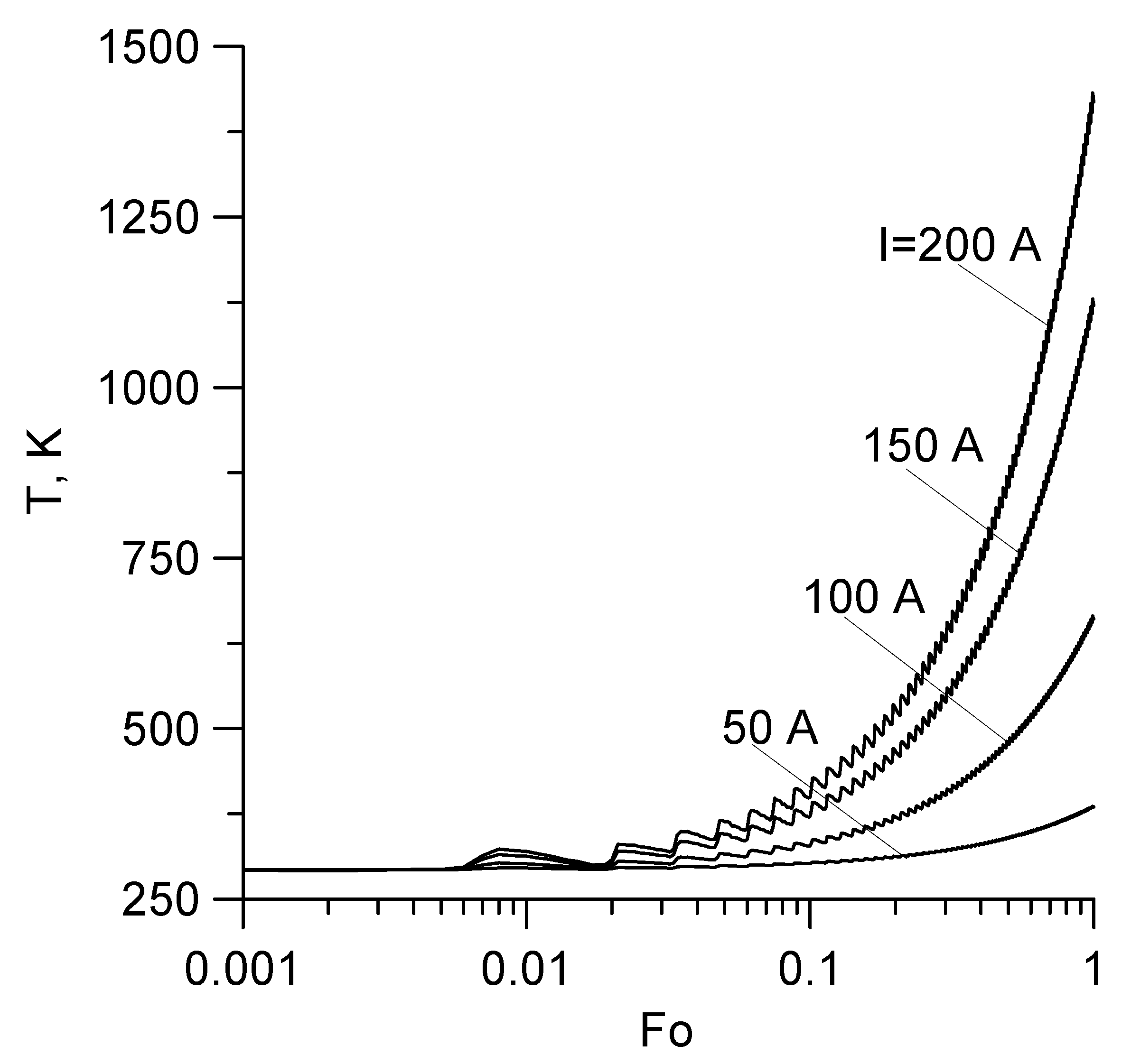
Figure 2 shows the temperature level depending on the Fourier number at the point ξ = 0.5, θ = 0°, ζ = 0.5 for different values of the current I. It is evident from the graph that at Fo < 0.1 the temperature is practically constant, but when Fo > 0.1 the picture changes, namely, the temperature increases in direct proportion to the time (here, the value Fo = 1 corresponds to τ = 26.6 min).

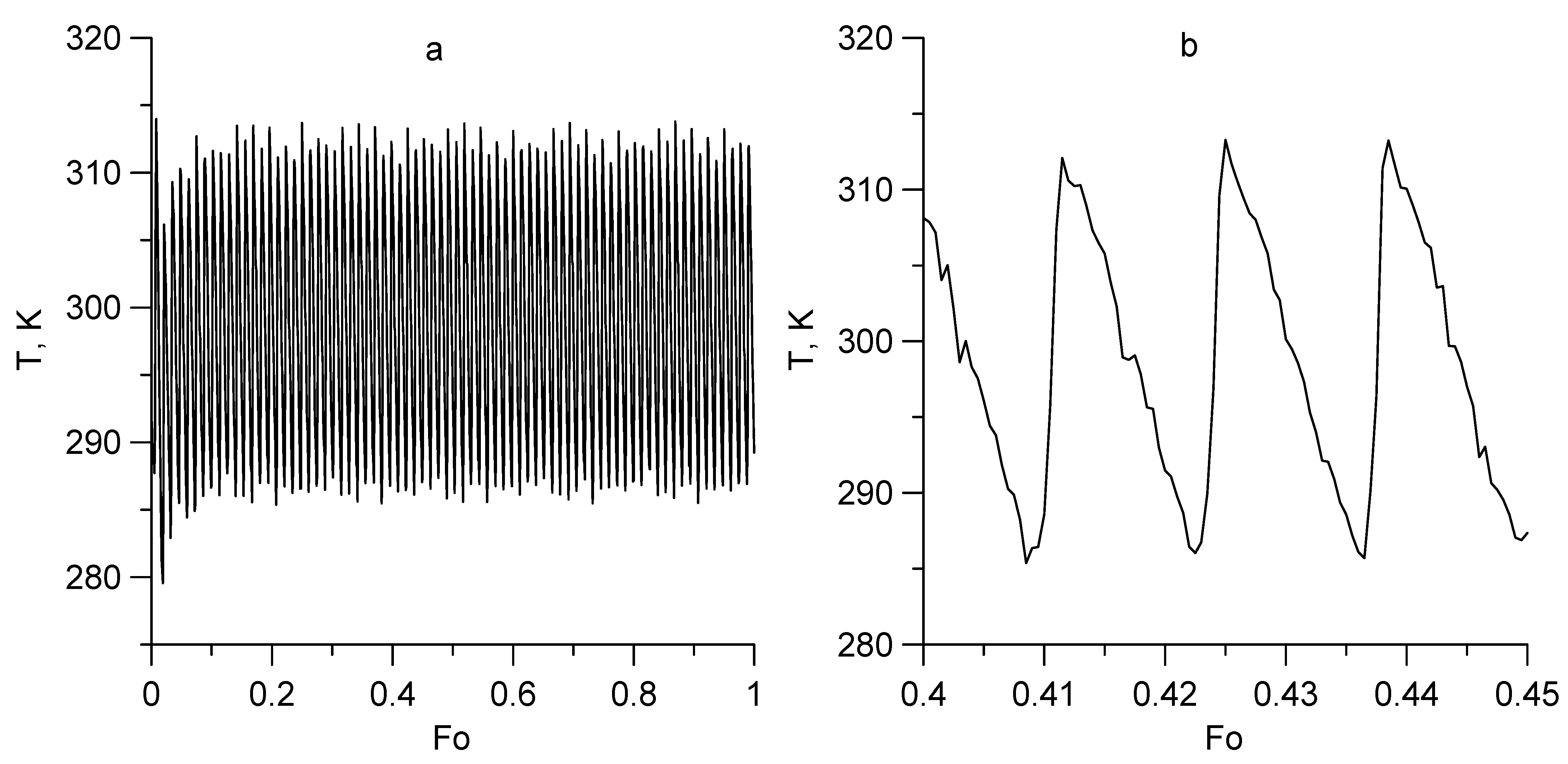
Figure 3 illustrates the same temperature (a) and its fragment (b) at I = 173 A, but without the component proportional to the Fourier number Fo. The selected value of the current I was found on the basis of experimental measurements of the temperature T* = 1123.15 K at the moment of time τ* = 20 min (Fo* ≈ 0.75) [11] according to the formula

$$T^{*}\approx T_0+\frac{q_0\epsilon \left(\epsilon +{\epsilon }_0\right)}{2\pi \lambda \left(1-{\epsilon }_0^2\right)\cos {\phi }_0}{\mathrm{Fo}}^{*},$$

(45)

that is

$$\mathrm{I}\approx \frac{S}{R_1}\sqrt{\frac{2\pi \lambda \left(T^{*}-T_0\right)\left(1-{\epsilon }_0^2\right)\cos {\phi }_0}{\epsilon \left(\epsilon +{\epsilon }_0\right){\rho }_0{\mathrm{Fo}}^{*}}}=173.1\mathrm{A}.$$

(46)

The characteristic non-monotonicity of the temperature over time should be noted. In addition, the temperature function is an amplitude-modulated signal (Figure 3a). The fine structure of the signal reveals its quasi-periodicity, and its shape is saw-toothed, with an amplitude of about 40 K (Figure 3b). The Fourier number, equivalent to the oscillation period (the rotation period of the screw), in this case is Fo₀ = 0.0135.

For a detailed analysis of the biomass heating in the reactor, we present the results of calculations of temperature changes over time at different points of the reactor. In the calculations of the local part of the temperature, that is, without the term proportional to time, it is advisable to exclude the dependence on the intensity of Joule heat. This can be achieved by focusing on the study of the so-called influence function ϑ = (T–T₀)/(q₀/πλ), which describes the effect on temperature of the screw’s geometry and angular velocity, as well as thermophysical parameters and the biomass flow rate

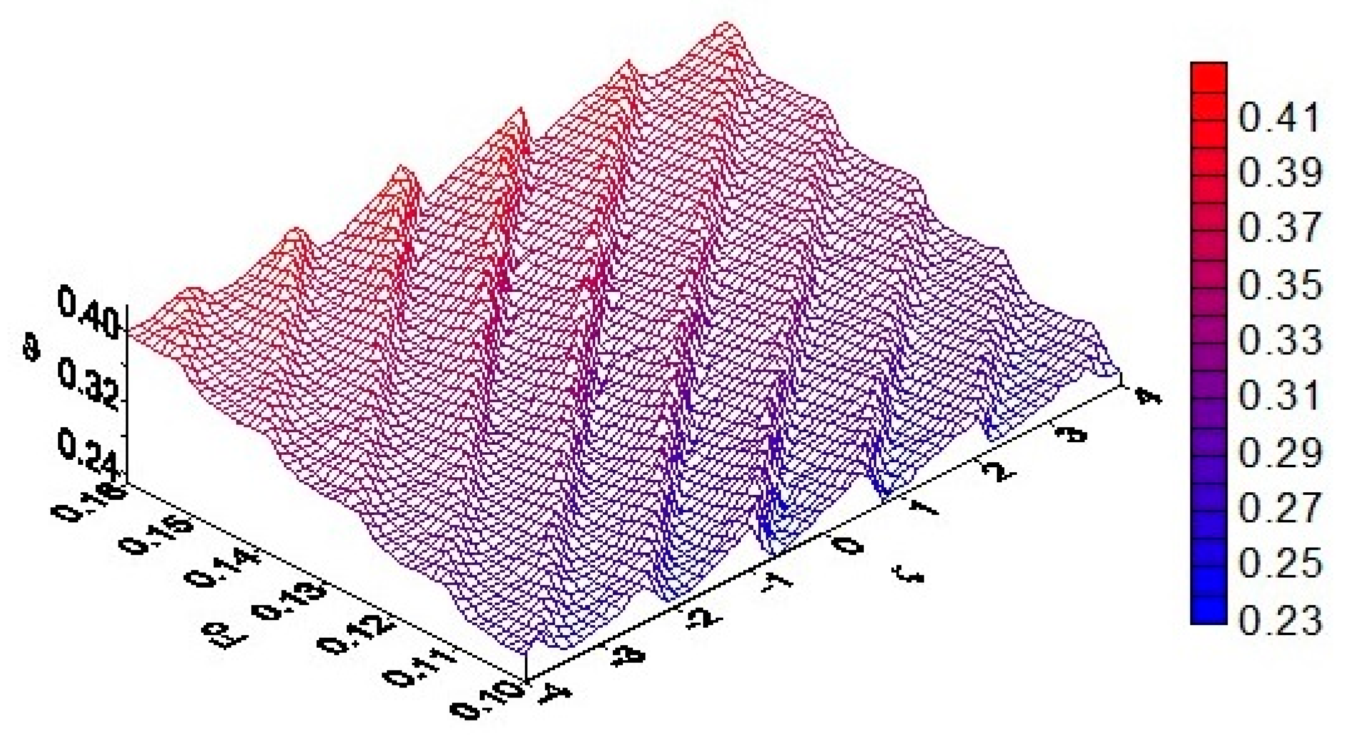
Figure 4 illustrates the time change of function ϑ on the rays ε₀ ≤ ξ ≤ 1, θ = 0°, ζ = 0.5. Here, the range of the Fourier number Fo corresponds to four periods of rotation of the auger and q₀/(πλ) = 435 K. It is shown that the influence function increases stepwise with time. Due to the spatial asymmetry of the heat source, the steps are inclined relative to the radial coordinate. During the transition of radial coordinate ξ from the inner surface of the channel to the outer surface, the amplitude of this function ϑ gradually decreases.

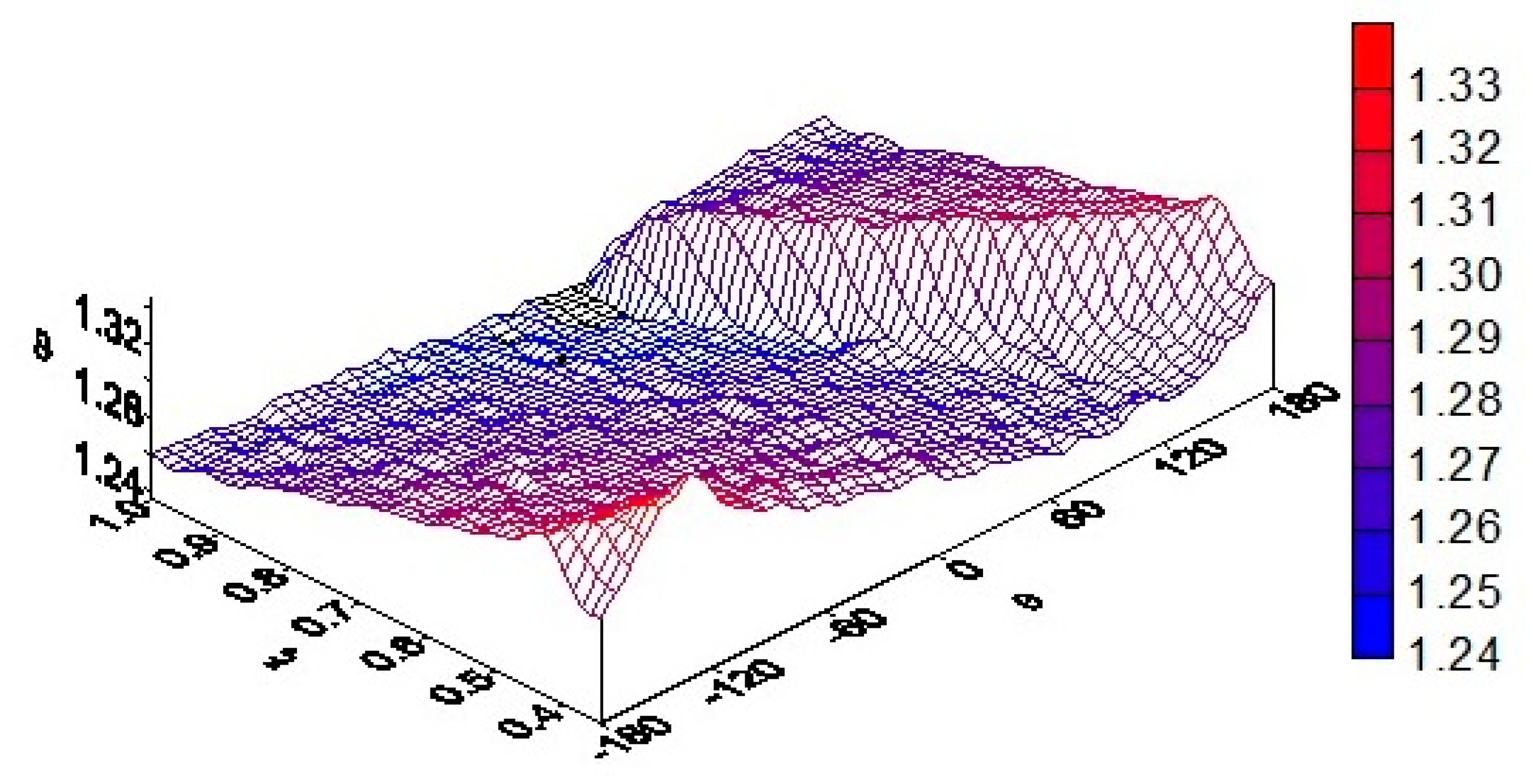
Figure 5 shows the angular dependence of the function ϑ on the circle ξ = 0.8, 0 ≤ |θ| ≤ 180°, ζ = 0.5 during four periods of screw rotation. The calculations show that in this case the influence function has a stepwise effect, and the steps are inclined relative to the angular coordinate. This function is also almost constant on the plateau surface, i.e., in the cross-sections of the channel returned to the axis of symmetry at an angle π/2–φ₀.

Figure 6 illustrates the axial distribution of the influence function ϑ along generating line of the cylindrical surface ξ = 0.8, θ = 0° on the four dimensionless pitches of the screw 0 ≤ |ζ| < 2Δ, Δ = 2πεcotφ₀ and for four periods of screw rotation. It is evident that the temperature gradually increases with time. As can be seen, along the Oz axis, the temperature amplitude has sawtooth cyclic ridges. The period of repetition of these ridges coincides with the dimensionless pitch of the screw. Additionally, in this case, the spatial-temporal distribution of the temperature has the character of periodic elongated plateaus, each of which is inclined at an angle φ₀ to the axis Oz.

Figure 7 shows the distribution of the function ϑ along the channel cross-section for ζ = 0.5 at a fixed moment of time. In this case, the temperature first increases as it approaches the outer surface of the channel, and then its value becomes almost constant and even slightly decreases. One characteristic is the transition of the temperature to a raised plateau, which is observed where the surface of the auger is located at the moment of time (in this case, at 60° < θ < 180°). This plateau changes its location over time.

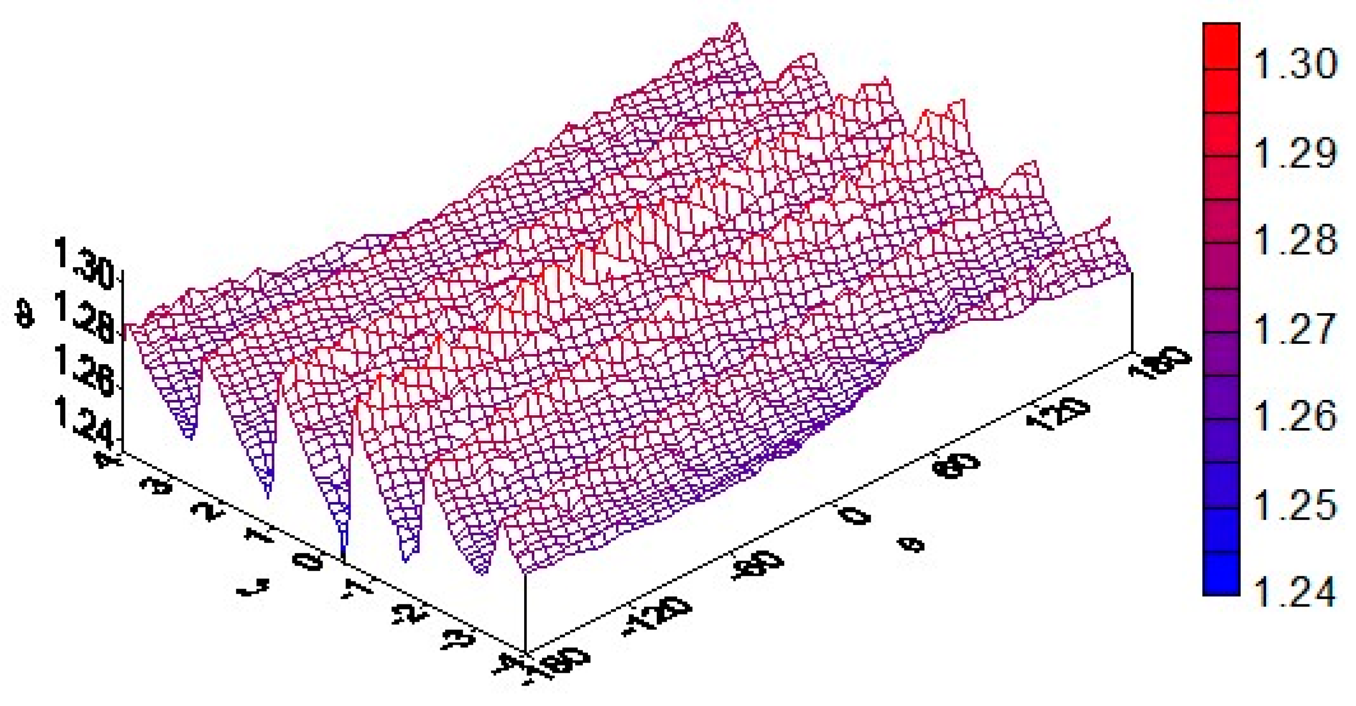
A completely different instantaneous temperature distribution is observed in the plane of the longitudinal section of the channel θ = 0° (Figure 8). Here, the calculations are performed within four dimensionless screw steps 0 ≤ |ζ| ≤ 4 at Fo = 0.5. The temperature field here is highly heterogeneous. The frequent oscillation in the amplitude of the function ϑ is associated with a change in the phase of the temperature fluctuations during rotation of the screw.

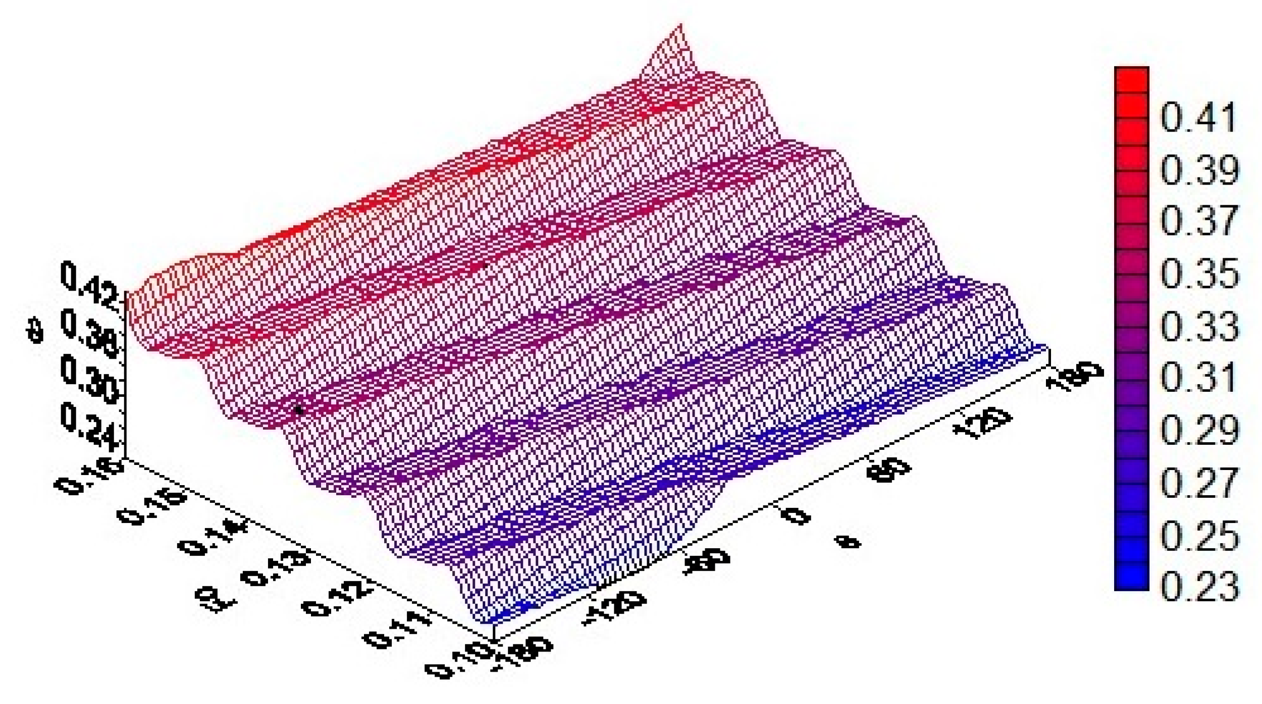
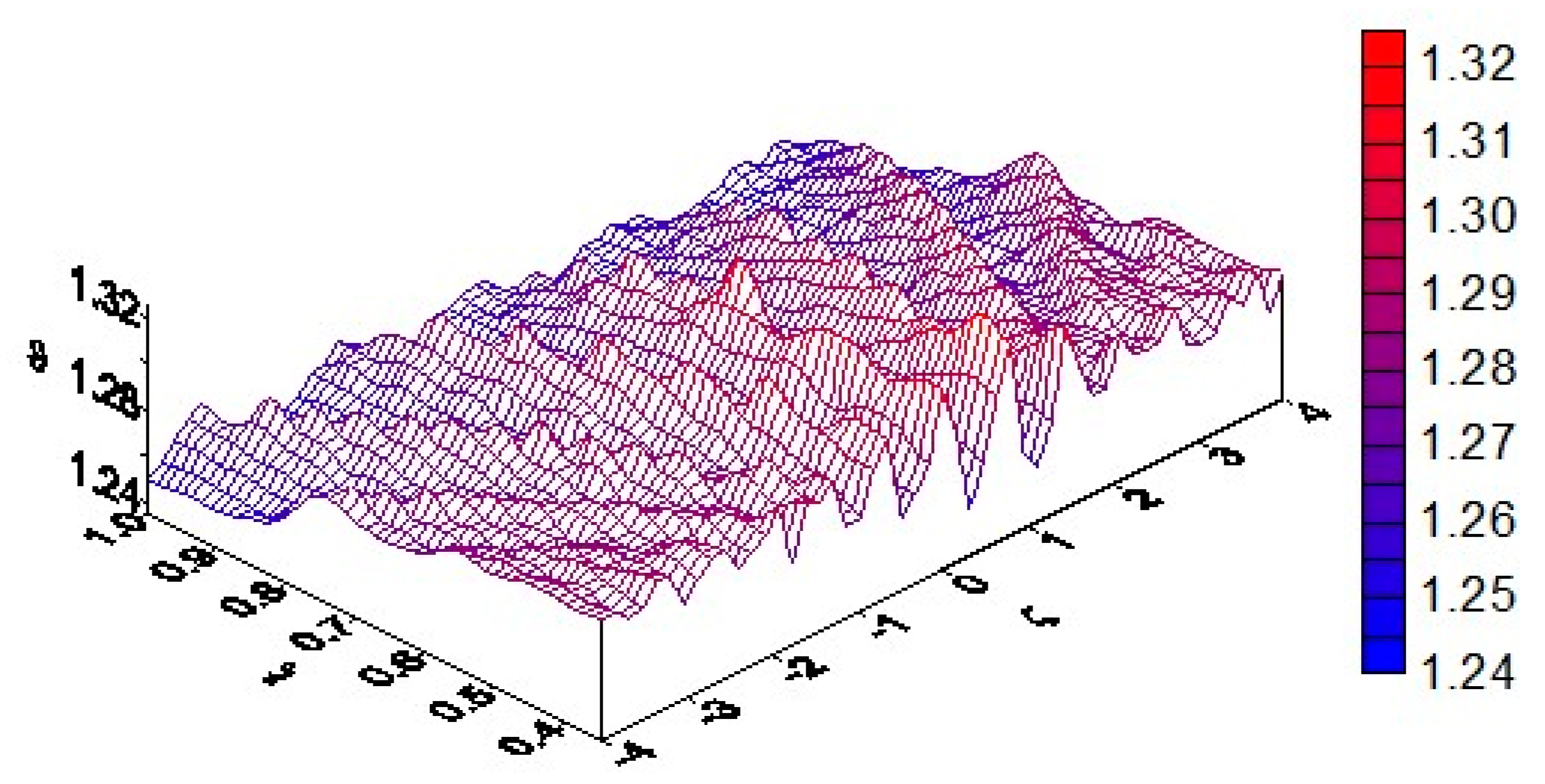
A more ordered distribution of the temperature field on the cylindrical surface ξ = 0.8, 0 ≤ |θ| ≤ 180°, 0 ≤ |ζ| ≤ 4 inside the channel at Fo = 0.5 is observed in Figure 9. It is characteristic that the amplitudes of the temperature fluctuations here resemble the profiles of a screw. Here, the temperature as a function of the axial coordinate ζ is also quasi-periodic (oscillation amplitude ϑ ≈ 0.04). At the same time, the temperature level remains almost constant on the ridges inclined to the axis of the channel at an angle φ₀.

Above, we analyzed the local temperature field for which the geometric and kinematic parameters of the system did not change. However, it is also interesting to evaluate the studied characteristics when the angular speed of rotation of the screw and its width are changing. It is known that a variation of the speed (or frequency) of screw rotation enables flexible adjustments of the residence time of biomass particles inside the screw reactor [15,24]. Therefore, it is important to evaluate the resulting temperature field.

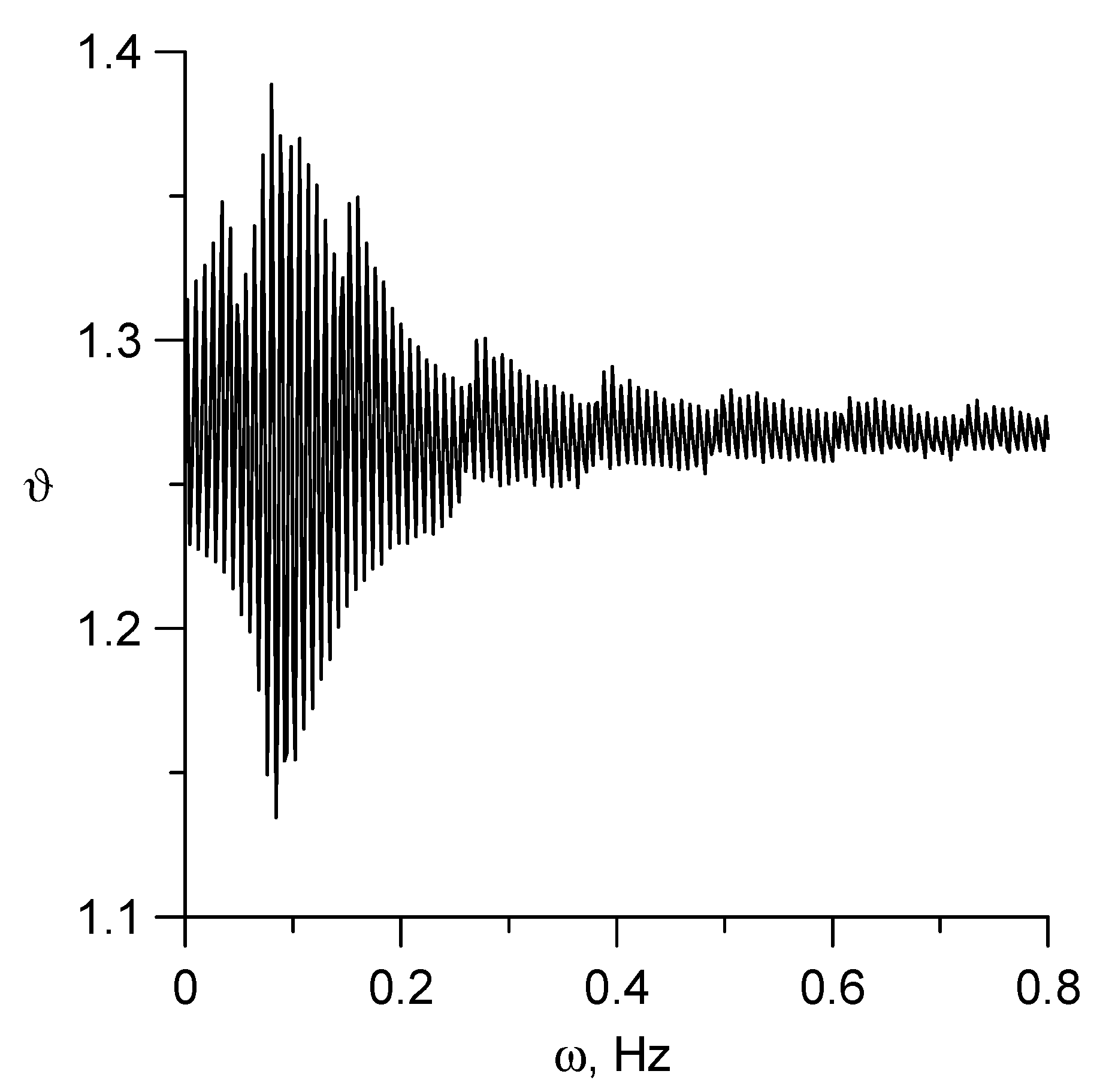
Figure 10 reflects this situation when the influence function ϑ is calculated at the point ξ = 0.8, θ = 0°, ζ = 0.5 for the Fourier number Fo = 0.5 at fixed values of φ₀ = 73.68° and v₀ = 5.89·10⁻⁴ m/s. It is evident that the temperature is an amplitude-modulated function of the angular velocity of the rotation of the screw. Moreover, an increase in the angular velocity ω leads to a damping effect on the temperature. The calculations also show that at the screw speed ω = 0.08 Hz, the temperature passes through the amplitude resonance. At a given axial velocity of the biomass, this is the value of the rotational speed that satisfies the condition of spatial synchronism.

ξFo_v= Fo₀, or v = ξR₀ω = v₀ξtanφ₀ (ε₀ ≤ ξ ≤ ε),

(47)

in which the vector of linear velocity of rotation of the point on the surface of the auger is equal to the projection of the velocity vector of biomass in the reactor. After passing the resonance, the amplitude of the temperature fluctuations slowly decreases.

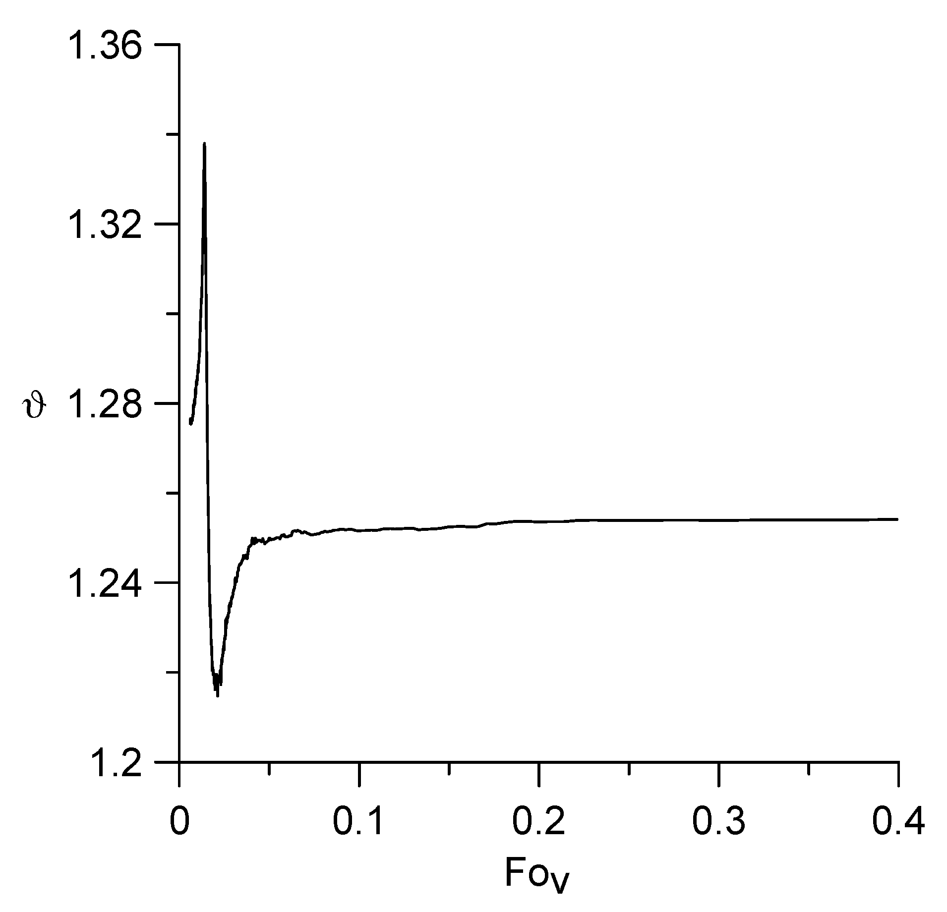
A similar resonant property of the function ϑ occurs when the linear velocity of the biomass v₀ (the dimensionless Fourier number Fo_v) changes, while the value of the angular velocity ω is unchanged. From Figure 11 it follows that at small values of Fo_v, the function ϑ reaches extreme values with a change of phase, i.e., the phase resonance of the temperature field is observed. In this case, the signal amplitude at Fo_v = 0.0140 is the maximum and at Fo_v = 0.0199 is minimal. Since Fo₀/ε = 0.0135/0.962 = 0.0140, this means that the condition of spatial synchronism (47) is satisfied at ξ = ε.

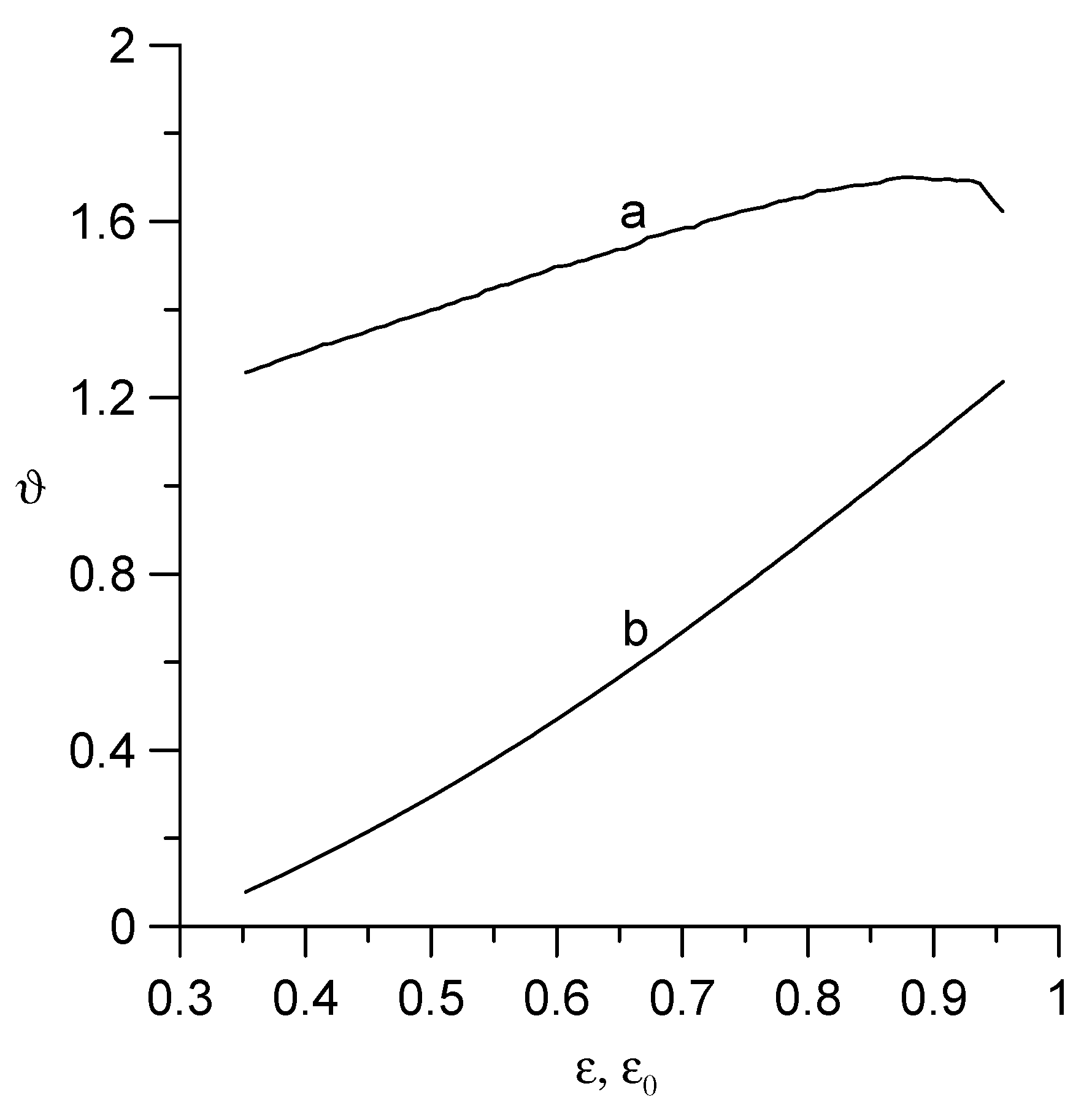
It is also interesting to investigate the dependence of the temperature field on the geometric dimensions of the heat source, because in the processing of biomass, raw materials with particles of different shapes, sizes, and morphological properties the shape of the helical screw play an important role [15,24]. The corresponding results of the calculations are shown in Figure 12. Here, curve (a) illustrates the dependence of the function ϑ on the dimensionless inner radius of the channel ε₀ at a fixed outer radius of the screw (ε = 0.962), and curve (b) depicts the dependence of this function on the dimensionless outer radius of the screw ε at a fixed inner radius of the channel (ε₀ = 0.346). In both cases, the calculations were performed at the channel point ξ = 0.8, θ = 0°, ζ = 0.5 for Fo = 0.5, ω = 0.292 Hz, v₀ = 5.89·10⁻⁴ m/s. As can be seen, the function ϑ increases monotonically with the increasing screw width. It should be noted that with a change in the parameters ε and ε₀, the current I changes and, accordingly, the total temperature T changes.

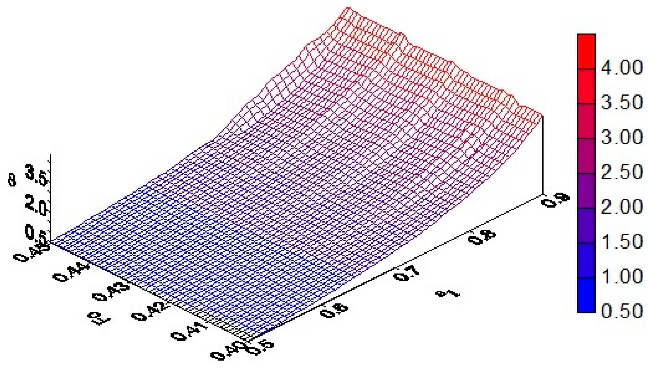
Figure 13 illustrates the dynamic effect of “scanning” noted in [16]. This phenomenon occurs when the screw of relative width Δ = ε – ε₀ moves from the inner surface of the channel to its outer surface (here, ε = ε₁ + 0.5Δ, ε₀ = ε₁ – 0.5Δ and). Therefore, in the periodic moments of time when the surface of the auger passes near the observation point, the amplitude of the influence function ϑ locally increases.

5. Conclusions

The article presents new mathematical modeling results of the heat transport process from the surface of an electrically heated screw, mounted on an axially rotating shaft, to the biomass transported in a thermally insulated channel. In reality, reactors have a finite length, but they are usually very long compared to the size of their cross-section. It is hoped that the temperature field at points far from the edges of the reactor will be weakly dependent on these edges, so in the first approximation the channel can be considered infinitely long. This greatly simplifies the problem statement and its solution. According to this assumption, the exact solution of the corresponding boundary value problem of mathematical physics is found in the form of the expansions of the given and required functions into Fourier series over an angular coordinate and integral Fourier and Laplace transforms over an axial coordinate and time, respectively. As a result, the temperature in the rector is obtained as the product of the function of the energy source, which is determined by the Joule heat and some function of influence. This last function is represented by the sum of the expressions, describing the global temperature field, which is directly proportional to time, and the Fourier–Bessel series, which simulates the microstructure of the temperature field. The influence function depends on the physicochemical parameters of the biomass, on the geometrical parameters of the screw (internal and external radii and its pitch), and on the angular rotation velocity of shaft. The components of the series include the coefficients in the form of the definite integral. The high-precision Romberg numerical method was used to calculate the value of this integral. Using the parameter values taken from real experiments, the following conclusions can be drawn from the results obtained during the calculations.

• As in the case of the heater in the form of a helix [16] or a shaftless screw [17], the temperature field in the channel with the screw mounted on the shaft is determined by the Joule heat, which increases in direct proportion to the operation time of the heat source; however, it is influenced by the geometry of the cross-section of the reactor.
• However, the temperature, which is globally determined by the Joule–Lenz effect, also has a fine structure. The latter does not depend on the intensity of the Joule heating and is formed locally under the influence of auger parameters (angular velocity, pitch, and outer and inner diameters) and depends slightly on the speed of the biomass. The fine structure of the temperature is described by a function of influence, which mathematically is represented by the integral over the dimensionless radial width of the screw.
• With the help of numerical calculations, it was established that due to the asymmetry of the heat source, which is a rotating screw, the temperature in the reactor undergoes sinusoidal amplitude-modulated oscillations that have a sawtooth shape. The period of these local oscillations of temperature is determined by the angular velocity of the screw.
• Comparing the obtained numerical results with those corresponding to the case of heat sources in the form of a helix [16] or a screw [17] without an axial shaft, we note the general similarity of the spatial-temporal temperature behavior in a cylindrical channel. However, the presence of an additional surface of the inner shaft significantly affects the formation of a fine structure of the spatial-temporal characteristics of the temperature. In particular, due to interference processes caused by the reflection of heat flows on two cylindrical surfaces, the local part of the temperature field becomes more amplitude-modulated.
• It was found that when the screw rotation frequency changes, the amplitude of the influence function passes through resonance. This resonant frequency of rotation of the auger is related to the axial velocity of the biomass in the channel due to the condition of spatial synchronism. A similar phenomenon of resonance is also observed in the phase change of the influence function, which occurs when the biomass’ movement speed changes, but the screw rotation speed is constant.

The calculation results indicate that the temperature field in the reactor in an initial time, commensurate with the time of the chemical reactions of the pyrolysis process, is quite heterogeneous in time and space. This fact should be known both by experimenters during the start-up of the pyrolysis process, and by developers of the processes of pyrolysis, sterilization and pasteurization of food products.

References

1. Piersa, P.; Unyay, H.; Szufa, S.; Lewandowska, W.; Modrzewski, R.; Slęzak, R.; Ledakowicz, S. An extensive review and comparison of modern biomass torrefaction reactors vs. biomass pyrolysis–Part 1. Energies 2022, 15, 2227. [Google Scholar] [CrossRef]
2. Campuzano, F.; Brown, R.C.; Martinez, J.D. Auger reactors for pyrolysis of biomass and wastes. Renew. Sustain. Energy Rev. 2019, 102, 372–409. [Google Scholar] [CrossRef]
3. Biogreen, The Pyrolyzer Spirajoule®. Available online: http://www.biogreen-energy.com/biogreen/spirajoule/2016 (accessed on 7 February 2016).
4. ETIA Ecologies, Thermal Processing of Bulk and Powders Powered by Electricity. 2019. Available online: https://etia-group.com/operations-for-thermal-processing (accessed on 3 February 2021).
5. Luz, F.C.; Cordiner, S.; Manni, A.; Mulone, V.; Rocco, V. Biomass fast pyrolysis in a shaftless screw reactor: A 1-D numerical model. Energy 2018, 157, 792–805. [Google Scholar] [CrossRef]
6. Luz, F.C.; Cordiner, S.; Manni, A.; Mulone, V.; Rocco, V. Biomass fast pyrolysis in screw reactors: Prediction of spent coffee grounds bio-oil production through a monodimensional model. Energy Convers. Manag. 2018, 168, 98–106. [Google Scholar] [CrossRef]
7. Cordiner, S.; Manni, A.; Mulone, V. Biomass fast pyrolysis in a shaftless screw reactor: Residence time distribution and heating up evaluation by means of a DEM approach. Comput. Therm. Sci. 2018, 10, 375–388. [Google Scholar] [CrossRef]
8. Henan Pingyuan Mining Machinary, Co. Ltd. What Factors That Affect the Screw Conveyor Conveying Efficiency? 2015. Available online: http://www.pkmachinery.com/faq/factors–affect–screw-conveyor-conveying-efficiency.html (accessed on 20 August 2016).
9. Yang, H.; Kudo, S.; Kuo, H.-P.; Norinaga, K.; Mori, A.; Mašek, O.; Hayashi, J. Estimation of enthalpy of bio-oil vapor and heat required for pyrolysis of biomass. Energy Fuels 2013, 27, 2675–2686. [Google Scholar] [CrossRef]
10. Available online: https://etia-group.com/our-products/spirajoule/ (accessed on 30 March 2022).
11. Ledakowicz, S.; Stolarek, P.; Malinowski, A.; Lepez, O. Thermochemical treatment of sewage sludge by integration of drying and pyrolysis/autogasification. Renew. Sustain. Energy Rev. 2019, 104, 319–327. [Google Scholar] [CrossRef]
12. Lepez, O.; Sajet, P. Device for the Thermal Processing of Divided Solids EP 2218300 A2 20100818 (FR). WO2009095564A2, 6 August 2009. [Google Scholar]
13. Shi, X.; Ronsse, F.; Roegiers, J.; Pieters, J.G. 3D Eulerian–Eulerian modeling of a screw reactor for biomass thermochemical conversion. Part 1: Solids flow dynamics and back-mixing. Renew. Energy 2019, 143, 1465–1476. [Google Scholar] [CrossRef]
14. Shi, X.; Ronsse, F.; Roegiers, J.; Pieters, J.G. 3D Eulerian–Eulerian modeling of a screw reactor for biomass thermochemical conversion. Part 2: Slow pyrolysis for char production. Renew. Energy 2019, 143, 1477–1487. [Google Scholar] [CrossRef]
15. Nachenius, R.W.; van de Wardt, T.A.; Ronsse, F.; Prins, W. Torrefaction of pine in a bench-scale screw conveyor reactor. Biomass Bioenergy 2015, 79, 96–104. [Google Scholar] [CrossRef]
16. Piddubniak, O.; Ledakowicz, S. Modeling of heat transfer from an electrically heated rotating helix in a circular cylindrical channel filled with a biomass moving at a constant velocity. Therm. Sci. Eng. Prog. 2022, 30, 101265. [Google Scholar] [CrossRef]
17. Ledakowicz, S.; Piddubniak, O. Analysis of non-stationary temperature field generated by a shaftless screw conveyor heated by Joule–Lenz effect. Chem. Process Eng. 2021, 42, 119–137. [Google Scholar] [CrossRef]
18. Carslaw, H.S.; Jaeger, J.C. Conduction of Heat in Solids; Clarendon Press: Oxford, UK, 1959. [Google Scholar]
19. Luikov, A.V. Analytical Heat Diffusion Theory; Acad. Press: New York, NY, USA, 1968. [Google Scholar]
20. Korn, G.A.; Korn, T.U. Mathematical Handbook for Scientists and Engineers: Definitions, Theorems and Formulas for References and Review; Dover Publ., Inc.: Mineola, NY, USA, 2000. [Google Scholar]
21. Krein, S.G. (Ed.) Functional Analysis; Wolters-Noorhoff Publ.: Groningen, The Netherlands, 1972. [Google Scholar]
22. Abramowitz, M.; Stegun, I.A. (Eds.) Handbook of Mathematical Functions with Formulas, Graphs, and Mathematical Tables; Dover Publ., Inc.: New York, NY, USA, 1972. [Google Scholar]
23. Prudnikov, A.P.; Brychkov, Y.A.; Marichev, O.I. Integrals and Series. Volume 1: Elementary Functions; Gordon and Breach Sci. Publ.: New York, NY, USA, 1986. [Google Scholar]
24. Nachenius, R.W.; Van De Wardt, T.A.; Ronsse, F.; Prins, W. Residence time distributions of coarse biomass particles in a screw conveyor reactor. Fuel Process. Technol. 2015, 130, 87–95. [Google Scholar] [CrossRef]
25. Press, W.H.; Teukolsky, S.A.; Vetterling, W.T.; Flannery, B.P. Numerical Recipes in Fortran 77: The Art of Scientific Computing; Volume 1 of Fortran numerical recipes; Cambridge Univ. Press: Cambridge, UK, 1992. [Google Scholar]
26. Burden, R.L.; Faires, J.D. Numerical Analysis; Brooks/Cole, Cengage Learning: Boston, MA, USA, 2010. [Google Scholar]
27. Available online: http://perso.orange.fr/jean-pierre.moreau/Fortran/tromberg_f90.txt (accessed on 24 August 2022).
Figure 1. The scheme of the auger with a shaft and the sizes of its section.
Energies 15 06164 g001
Figure 2. The temperature at the point ξ = 0.5, θ = 0°, ζ = 0.5 at different values of the Fourier number and current I.
Energies 15 06164 g002
Figure 3. Temperature (a) and its image on a larger scale (b) at different moments of time at the point ξ = 0.8, θ = 0°, ζ = 0.5 for I = 173 without taking into account the linear term proportional to Fo.
Energies 15 06164 g003
Figure 4. The temperature distribution along the ray ε0ξ ≤ 1, θ = 0, ζ = 0.5 for four periods of oscillation.
Energies 15 06164 g004
Figure 5. The angular distribution of the temperature on the circle ξ = 0.8, 0 ≤ |θ| ≤ 180°, ζ = 0.5 for four periods of screw rotation.
Energies 15 06164 g005
Figure 6. The axial distribution of the temperature along the generatrix of cylinder of the helix ξ = 0.8, θ = 0° during four periods of screw rotation.
Energies 15 06164 g006
Figure 7. The 3-D radial-angular instantaneous distribution of function ϑ in the cross-section ζ = 0.5.
Energies 15 06164 g007
Figure 8. The 3-D radial-axial instantaneous distribution of function ϑ in the plane ε0ξ ≤ 1, 0 ≤ |ζ| ≤ 4 at θ = 0° and Fo = 0.5.
Energies 15 06164 g008
Figure 9. The 3-D axial-angular instantaneous distribution of function ϑ on the surface 0 ≤ |θ| ≤ 180°, 0 ≤ |ζ| ≤ 4 for ξ = 0.8 and Fo = 0.5.
Energies 15 06164 g009
Figure 10. The local temperature ϑ as function of angular velocity of rotation of the screw at the point ξ = 0.8, θ = 0°, ζ = 0.5, Fo = 0.5 for φ0 = 73.68° and v0 = 5.89 × 10⁻⁴ m/s (Fov= 0.593).
Energies 15 06164 g010
Figure 11. The local temperature ϑ as function of Fourier number corresponding to the flow rate of the substance v0 at the point ξ = 0.8, θ = 0°, ζ = 0.5 for Fo = 0.5, φ0 = 73.68°, ω = 0.292 Hz (Fo0 = 0.0135) and R2 = 0.009 m.
Energies 15 06164 g011
Figure 12. Temperature as a function of the relative radius of the auger shaft ε0 (a) and the outer radius of the auger ε (b) at the point ξ = 0.8, θ = 0°, ζ = 0.5 for Fo = 0.5, φ0 = 73.68°, ω = 0.292 Hz, v0 = 5.89 × 10⁻⁴ m/s.
Energies 15 06164 g012
Figure 13. The dependence of temperature on parameter ε1 at the point ξ = 0.8, θ = 0°, ζ = 0.5 пpи φ0 = 73.68°, ω = 0.292 Hz, v0 = 5.89 × 10⁻⁴ m/s.
Energies 15 06164 g013