Abstract
Hot dry rock (HDR) geothermal energy, as a clean and renewable energy, has potential value in meeting the rapid demand of the social economy. Predicting the temperature distribution of a subsurface target zone is a fundamental issue for the exploration and evaluation of hot dry rock. Numerical finite–element simulation is currently the mainstream method used to study the variation in underground temperature fields. However, it has difficulty in dealing with multiple geological elements of deep and complex hot dry rock models. A Unity networking for hot dry rock temperature (HDRT–UNet) is proposed in this study that incorporates the matrix rock temperature field equation for relating the three parameters of density, specific heat capacity and thermal conductivity. According to the numerical geological structures and rock parameters of cap rocks, faults and magma intrusions, a new dataset simulated by the finite element method was created for training the HDRT–UNet. The temperature simulation results in the Gonghe basin show that the predicted temperatures within faults and granites were higher than their surrounding rocks, while a lower thermal conductivity of the cap rocks caused the temperature of overlying strata to be smaller than their surrounding temperature field. The simulation results also prove that our proposed HDRT–UNet can provide a certain evolutionary knowledge for the prediction and development of geothermal reserves.
1. Introduction
Geothermal energy is a kind of clean and renewable energy in deep strata, and it is one of the alternatives to fossil fuels such as coal, oil and natural gas [1]. Geothermal energy has the advantages of large reserves, broad distribution, good stability and high utilization efficiency. Hot dry rock power generation technology can greatly reduce the impact of the greenhouse effect and acid rain on the environment, and it is not restricted by seasons and climates, so it can be developed and utilized all the time. The cost of using hot dry rock to generate electricity is only half that of wind power [2]. Geothermal energy is more stable and superior to wind power, solar power and tidal power. It also has more development potential [3]. However, predicting the evolution of formation temperature is the basis for evaluating the reserves of hot dry rock geothermal resources, calculating the development potential and designing the development plan [4]. Temperature field simulation of hot dry rock predominantly includes a numerical simulation and interpolation method. The available numerical simulation method lacks the theoretical formula to deal with complex models with multiple geological elements. The reliability of the interpolation method depends on the data coverage rate, which will increase the cost. Therefore, based on the in–situ measured temperature data and rock parameters, predicting the formation temperature field is a very challenging task.
A key distribution law of the temperature field can be provided for engineering practice through the numerical simulation of HDR geothermal energy. Researchers have explored various HDR simulation methods and conducted a large number of numerical simulation studies [5,6]. Blocher (2010) highlighted the importance of numerical simulation in geothermal research [7]. Zeng et al. (2013) investigated sensitive parameters based on logging data and numerical simulation [8]. Shi et al. (2018) researched the influence of key factors such as groundwater on geothermal systems with numerical simulation [9]. Zhang et al. (2021) surveyed the feasibility of extracting geothermal energy from hot dry rock by a 2500 m super–long gravity heat pipe by numerical simulation [10].
At present, the simulation of temperature fields is predominantly based on the finite element method (FEM). Feng et al. (2012) used the FEM to analyze the zonal temperature distribution [11]. Zhao et al. (2014) established a fractured reservoir model of HDR by the FEM, reviewed a formula of water temperature change according to the measured–fracture water temperature change and the fracture model, and used this formula to forecast the future water temperature change [12]. Wei et al. (2019) numerically simulated the changes in temperature, stress and seepage after the exploitation of the Yangbajing geothermal field in Tibet by the FEM [13]. Zeng et al. (2020) numerically studied the distribution of temperature field, pressure field and water density in the Zhangzhou geothermal field by using the FEM and analyzed the main factors affecting the temperature field, pressure field and water density [14]. Li et al. (2020) established the hydrodynamics and heat transfer model by the finite element software ANSYS fluent and studied the heat transfer between the heat exchange tube and the surrounding rock in the process of heat storage and extraction [15]. Chen et al. (2021) utilized the Finite Volume Method to solve a thermal–hydraulic–mechanical coupling model. Several numerical experiments were carried out and compared with commercial software to verify the feasibility of the method [16]. S. Üner and D. Dusunur (2021) created a complete hydrothermal geophysical model by implementing the finite volume code ANSYS fluent. In this model, the physical and thermal properties of existing rocks are used to compute and display the fluid velocity and temperature mode [17]. The embedded discrete fracture model (EDFM) directly divides the bedrock into structured grids, then embeds the fractures into the bedrock grid system, and forms the fracture grid according to the intersection with the bedrock. The extended finite element method (XFEM) is an effective numerical method for solving the discontinuous problem. Li et al. (2021) used the embedded discrete fracture model (EDFM) and the extended finite element method (XFEM) to analyze the distribution of pressure, temperature and displacement fields in EGS. A combination of the EDFM and the XFEM was proposed to reduce the number of grids, enhance the calculation efficiency and maintain a high accuracy [18]. Diego Viesi et al. (2022) used 3D finite element modeling to evaluate the thermal effect in the ground according to real cases, such as the Madonna Bianca neighborhood in the city of Trento [19].
Intelligent big–data processing requires a reasonable processing cycle, and HDR temperature numerical simulation needs to calibrate the numerical geothermal model with detailed geological structure information. This procedure usually depends on the experience of geothermal workers, a large number of parameter adjustments and repeated tests. As it is time–consuming and subjective work, it is urgent to explore a new intelligent HDR temperature simulation method. In recent years, a large number of machine–learning methods have been developed to automatically extract features and discover the relationship hidden in a large number of data, which is conducive to establishing a functional relationship between the temperature field and rock parameters [20]. In recent years, it has been increasingly used in geothermal research. Based on artificial neural network (ANN) predictive control, Gang et al. (2014) proposed a method of hybrid ground–source heat pump systems and compared them with the methods of schedule–based and temperature–differential–based control systems. [21]. Gradient Boosted Regression Tree (GBRT) is composed of several decision trees, and the output results of all the trees add up to be the final answer. Rezvanbehbahani et al. (2017) establish a complex relationship between geothermal heat flow (GHF) and the geologic–tectonic features using GBRT algorithm techniques and then predicted the GHF for the Greenland Ice Sheet [22]. Tut Haklidir and Haklidir (2020) used a deep neural network (DNN) and a traditional machine learning algorithm to predict geothermal fluid temperature. The results showed that the DNN algorithm had a better performance and more accurate prediction [23]. Maryadi M et al. (2021) used ANN combined with magneto–telluric technology to conduct geothermal exploration in Indonesia [24]. Vivas and Salehi (2021) established data sets and labels using drilling data and thermal conductivity, respectively, and evaluated the effects of four different supervised–regression algorithms in testing thermal conductivity, and finally concluded that a KNN (k—Nearest Neighbor algorithm) algorithm can better predict thermal conductivity, and subsequently applied this algorithm to actual data [25]. He et al. (2022) used the machine–learning method to predict geothermal heat flow in the Bohai Basin [26]. Yang et al. (2022) established the complex relationship between the identification factor and temperature by a depth–confidence network, and finally predicted the formation temperature [27]. The above studies show that machine learning is a feasible method for temperature prediction in hot dry rock geothermal areas.
In this study, we propose a HDRT–UNet method to resolve the issue of temperature simulation for deep complex hot dry rock. First, the HDRT–UNet model is introduced that contains a HDRT–UNet structure and parameter fusion. Second, we introduce the establishment of a temperature simulation data training set by classic numerical models, and two complex geological models are used to test the performance of the proposed method. Finally, we discuss the proposed method and analyze the influence of hyperparameters, training data sets and other aspects on our proposed method. The evolution law of temperature fields involved with fractures, caprocks and other factors is also investigated.
2. HDRT–UNet Methods
2.1. Review of Temperature Control Formula
There are many rock parameters that affect underground temperature fields [28,29]. In this paper, the relations of three key parameters (specific heat capacity, density, thermal conductivity) are determined according to the basic equations of temperature field control. The value range of the three parameters is quite huge, which has a great influence on network fitting. A physical relationship between thermal diffusivity and the three parameters is used to eliminate the influence of multi–parameter coupling and different value amplitudes.
Three basic equations of temperature field control are listed:
Mass conservation equation:
Momentum conservation equation:
Energy conservation equation:
where denotes thermal conductivity; is density; is speed; is time; is physical strength; , is pressure; is unit tensor; is viscous stress tensor; is specific heat capacity of rock; and is rock temperature.
Initial conditions:
where denotes the temperature at t time and in the position (x,y) under the initial conditions.
Dirichlet boundary conditions:
where denotes the temperature given on the boundary, ; are the boundary conditions of upper, lower, left and right boundaries of the model, respectively.
Assuming that there is no water in the hot dry rock and the heat exchange among the strata is conducted in the way of heat conduction, the flow rate is 0:
where .
2.2. HDRT–UNet Method for Temperature Field
In the simulation of the temperature field by the finite element method, the debugging of parameters and the personnel experience will have a great influence on the results. The UNet is a neural network consisting of a classical encoder–decoder framework to discover hidden features or patterns in data [30]. The UNet’s powerful nonlinear mapping ability can be used to explore a relationship between a temperature field and rock parameters and reduce the influence of parameter debugging and human factors. We propose a HDRT–UNet method for establishing the functional relationship between the thermal diffusivity and the temperature fields.
Figure 1 shows that the architecture of our HDRT–UNet model has an end–to–end framework. In order to fit to the data, we made two major modifications to the UNet. First, we changed the UNet three–channel input into a single channel. Secondly, in the UNet, the number of output and input channels is 3 channels of RGB. To complete our task, we changed the output layer and the input layer to 1. To accomplish our task, we change the number of channels in the output and input layers to 1.
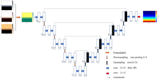
Figure 1.
The structure of HDRT–UNet.
The relationship between 2D temperature field and various physical parameters can be expressed as:
where represents the thermal diffusivity. It can be described as follows:
The HDRT–UNet takes a geological model of thermal diffusivity as an input, and the temperature field simulated by the finite element method serves as its expected output. This process can be expressed as:
where denotes an HDRT–UNet that indicates a nonlinear mapping of the network; , and are learnable parameters; represents a weight matrix; represents a bias matrix.
In the training process of the neural network, the objective function is continuously optimized and adjusted. By repeatedly comparing the difference between the current objective function and the expected objective function, the super parameters (weight and deviation) of each layer in the neural network are adjusted. Through the optimization and adjustment of the objective function, the error between the network temperature prediction and the expected temperature output is gradually reduced. We used the mean square error function to measure the error between and :
where the term represents the Frobenius norm; represents the number of training samples.
For updating the learned parameter , the optimization problem can be solved by using back propagation and adaptive moment estimation algorithms (Adam) [31].
where represents the neural network parameters of layer i, represents the learning rate.
The structure of the HDRT–UNet is shown in Figure 1. The HDRT–UNet is a network structure containing an encoder and decoder. A geological model of thermal diffusivity is set as an input, which is followed by the encoder. The encoder is composed of a convolutional layer and a pooling layer. After applying maxpool, the size of the feature maps is changed to half of the previous one. Then, there is the decoder, in which a transposed convolution operation is applied to amplify the output size to make it the same as the input geological model. Finally, the functional relationship between the temperature field and the formation thermal conductivity coefficient is gained through the convolution layer, pool layer and convolution layer, and the network simulation of the temperature field is realized.
The encoder includes a convolution layer and a down–sampling layer, and the operation performed by the convolution layer can be represented by the following formula:
where represents the characteristic diagram of layer K in the encoder; represents the Rectified Linear Unit; represents the Batch Normalization. In the convolution layer of the encoder, the feature map from the previous layer will be calculated twice according to Formula (10) (the convolution kernel size is 3 × 3 in convolution operation, and the convolution step size is 1), and the size of the feature map will be kept unchanged by zero padding. After the first convolution, the number of feature maps doubles, while the number of feature maps in the second convolution remains unchanged. The convolution layer is followed by the down–sampling layer, and the operations performed by the down–sampling layer can be expressed as:
where represents the down–sampling operation. The improved HDRT–UNet adopts a convolution operation with a convolution kernel of 4 × 4 and a convolution step size of 2 instead of maximum pooling, which increases the complexity of the network calculation and the consumption of the GPU. In order to reduce the large number of calculations, the maximum maxpool in the traditional HDRT–UNet is used for down–sampling.
The HDRT–UNet connects four concatenates between the encoder and decoder to fuse features of different scales, as shown in Figure 1. The decoder includes a convolution layer and an up–sampling layer. In the convolution layer of the decoder, the feature map from the upper layer is spliced with the feature map from the encoder by jumper wires, and the spliced feature map is used as the input of the convolution layer. The process can be expressed as follows:
where represents the characteristic diagram of layer in decoder; represents the characteristic diagram with the same number of channels as from the encoder; represents the splicing operation. The result of Formula (14) is subjected to a convolution operation as shown in Formula (12) again (convolution kernel size is 3 × 3, convolution step size is 1), and zero padding is performed to obtain the output result of the convolution layer in the decoder. After the first convolution, the number of feature maps is reduced to half of the original number, and the number of feature maps in the second convolution is unchanged. The convolution layer is followed by the sampling layer. After transposed convolution, the size of the feature map is doubled, and the number of feature maps is reduced to one half. In the last layer of the decoder, the functional relationship between the temperature field and the thermal conductivity coefficient is obtained by convolution with a convolution kernel with a size of 1 × 1. After the training of the HDRT–UNet, one can input the geological model that needs to simulate the temperature field, and the HDRT–UNet can realize the end–to–end temperature field simulation.
2.3. Data Set Preparation
As a data–driven algorithm, the performance of the proposed HDRT–UNet depends on the training data set. In order to explore the functional relationship between the temperature field and the thermal diffusivity, we used the formation parameters from petrophysical experiments of an actual underground structure to establish a geological model for the training data set by the finite element method. The following basic assumptions were proposed to establish the mathematical model in this study.
- The matrix rock block and the rock mass with faults were simplified as a continuous medium of homogenous isotropic elastomers.
- The rock mass was hot dry rock, and the factors such as water permeability and water storage of the rock block were neglected in the geological model. Since the rock radiation heat transfer was complicated to deal with, only conduction heat transfer was considered.
- There was no heat source in the geological model, and the deep mantle heat was considered as the boundary of the model when initial conditions were set.
For the training data set, we established a 2D geological model containing density, thermal conductivity and specific heat capacity. The parameters of the rock mass are listed in Table 1. The geological model meets the above basic assumptions, and the size of each geological model was 16 × 16 km, the temperature of mantle heat source was 500 °C, and the ground temperature was 15 °C. Figure 2 shows 6 geological models from the training data set. When inputting the geological model into the neural network, we adjusted the relative position of the stratum to an absolute position. Figure 3, Figure 4, Figure 5 and Figure 6 show the density, specific heat capacity, thermal conductivity and calculated thermal diffusivity in the geological model. After the establishment of the geological model, we simulated the heat conduction of the model by the finite element method, calculated the temperature field after 100,000 years, and established the label of the training data as shown in Figure 7.

Table 1.
Rock mass parameters.
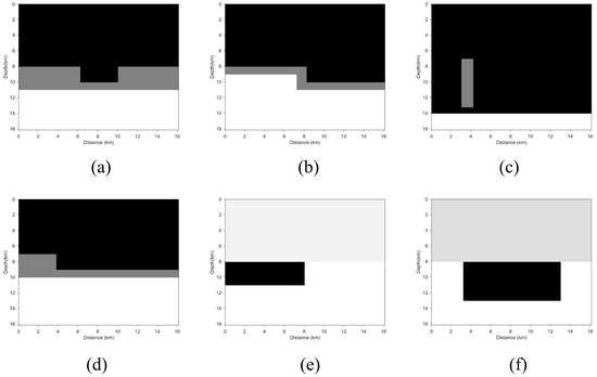
Figure 2.
The six randomly selected geological models (a–f) from the training data set, (a–f) the six geological models contain different geological structures: (a) Graben model, (b) pleated–structure model, (c) magmatic intrusion model, (d) platform model, (e) magmatic intrusion model, (f) magmatic intrusion model. Different geological models enrich the training data set.
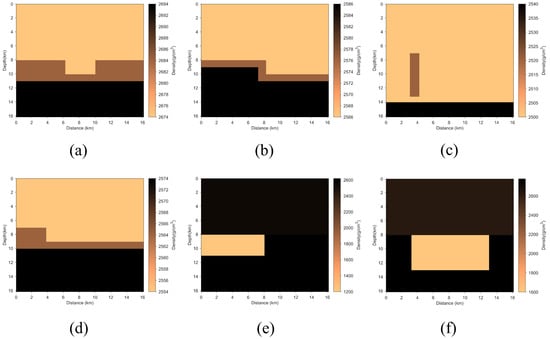
Figure 3.
The density parameters of six geological models (a–f) for the training data set: (a) Graben model, (b) pleated–structure model, (c) magmatic intrusion model, (d) platform model, (e) magmatic intrusion model, (f) magmatic intrusion model.
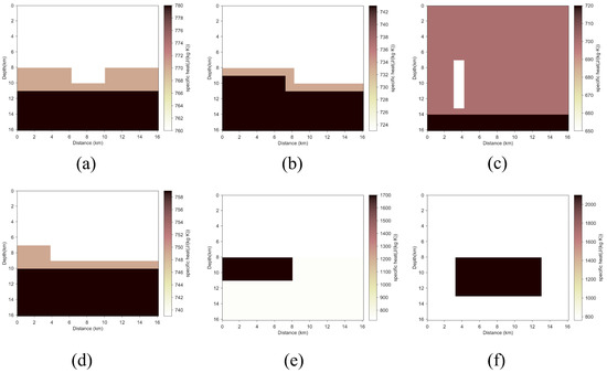
Figure 4.
Specific heat capacity of six geological models (a–f) for the training data set: (a) Graben model, (b) pleated–structure model, (c) magmatic intrusion model, (d) platform model, (e) magmatic intrusion model, (f) magmatic intrusion model.
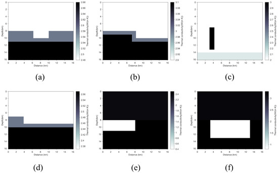
Figure 5.
Thermal conductivity of six geological models (a–f) for the training data set: (a) Graben model, (b) pleated–structure model, (c) magmatic intrusion model, (d) platform model, (e) magmatic intrusion model, (f) magmatic intrusion model.
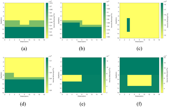
Figure 6.
The calculated thermal diffusivity of six geological models (a–f): (a) Graben model, (b) pleated–structure model, (c) magmatic intrusion model, (d) platform model, (e) magmatic intrusion model, (f) magmatic intrusion model.
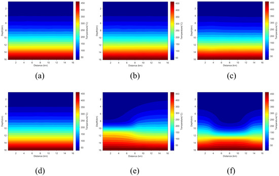
Figure 7.
The temperature field labels of six geological models (a–f) from the training data set. (a) Temperature field of Graben model, (b) temperature field of pleated–structure model, (c) temperature field of magmatic intrusion model, (d) temperature field of platform model, (e) temperature field of magmatic intrusion model, (f) temperature field of magmatic intrusion model. The finite element method was used to simulate the heat conduction of the model, the temperature field after 100,000 years was simulated, and the label was established.
Data preprocessing was used to reduce the influence of the numerical difference between the parameters of the model and decrease the fitting time of the HDRT–UNet. We used the normalization method to preprocess the formation parameters. The purpose of normalization is to process the data of different scales and dimensions, so that they can be scaled to the same data interval and range, so as to reduce the influence of the scale, characteristics and distribution differences on the model. If normalization is not carried out, the values of different features in the feature vector are quite different. When the gradient descends, the direction of the gradient will deviate from the direction of the minimum value, resulting in a too–long training time or network under–fitting. In this paper, the numerical value of thermal diffusion was reduced to the range of [0, 1] by the normalization method and input into the network. The normalization formula is:
where is the original formation parameters, is the maximum value of data, and is the normalized formation parameters.
In order to expand our training data, we cut the training data and tags into 160 × 160 slices, and we obtained 9000 slices and their corresponding tags. Among them, 7200 slices were used as the synthetic training data set of the network, and the other 1800 slices were used as the verification set.
2.4. Training the HDRT–UNet
We used 0.001 as the initial learning rate; the learning rate was attenuated using the cosine–annealing algorithm [32]. We selected 32 and 100 for the batch size and epoch, respectively. We used the Adam algorithm to optimize the learning objectives [31]. Figure 8 shows the change in the value of the loss function during network training. As shown in the figure, the loss value dropped rapidly in the epoch from 0 to 40, slowed down in the epoch from 40 to 80, and reached a lower value near the 80th epoch and tended to be steady.
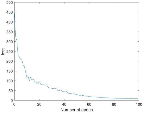
Figure 8.
The change in loss function value during training process: mean–squared error for the simulate temperature field.
3. HDR Mode Temperature Simulation
3.1. Two–Testing Geological Model
In this section, we test the effectiveness of the network based on the training data. We designed two geological models with a size of 16 × 16 km as shown in Figure 9. The geological model in Figure 9a contains the heat conduction channels and granite with high thermal conductivity, and the geological model in Figure 9b contains a heat conduction channel and a non–thermal conductive caprock. We simulated the temperature field by using the finite element method and HDRT–UNet, respectively, and the corresponding simulation results are shown in Figure 10 and Figure 11.
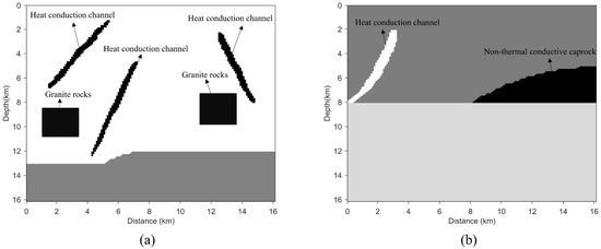
Figure 9.
Two–dimensional (2D) geological model. (a) The first model consist of the heat conduction channels and granite with high thermal conductivity; (b) The second model contains fractures and caprock.
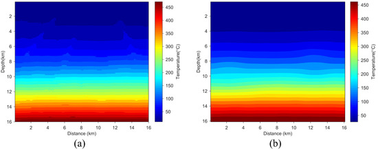
Figure 10.
Temperature simulation comparison of the first model. (a) Temperature field simulated by the HDRT–UNet; (b) Temperature field simulated by the finite element method.
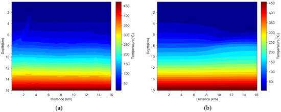
Figure 11.
Temperature simulation comparison of the second model. (a) Temperature field simulated by the HDRT–UNet; (b) Temperature field simulated by the finite element method.
Figure 10 shows the simulation of the temperature field of the geological model in Figure 9a by the finite element method and the HDRT–UNet. The results show that the simulation effect of the HDRT–UNet on the heat conduction channel and granite with good thermal conductivity was better than that of the finite element method. Figure 11 shows the simulation of the temperature field of the geological model in Figure 9b by the finite element method and the HDRT–UNet. The results show that the simulation effect of the HDRT–UNet on the heat conduction channel was better than that of the finite element method, and the effect of the finite element method on non–thermal conductive cover was more obvious. The HDRT–UNet also had a certain effect on cover, but no finite element software is sensitive to cover. These two geological models verify that the HDRT–UNet can simulate the temperature field, but the network needs to be improved to avoid the poor effect on the caprock in Figure 11.
3.2. Gonghe Geological Model
As the transitional zone between Qilian Mountain and Kunlun Mountain (Figure 12), the Gonghe Basin has the advantages of wide distribution, good lithological conditions and abundant hot dry rock resources [33]. The high–temperature mass drilled in Gonghe Basin is the first large–scale available hot dry rock resource with a temperature above 200 °C. There are many cap rocks, faults and magma intrusions in the Gonghe Basin [34]. In terms of stratum, the Gonghe area is mainly dominantly covered by thick Cenozoic deposits, including mudstone, sandy mudstone, sandstone and glutenite in the Quaternary, Neogene and Paleogene strata [35]. Triassic formations and Indosinian acidic magmatic rocks are also present [36].
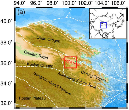
Figure 12.
The distribution of major tectonic structures in Gonghe Basin [37].
To further show the outstanding ability of the proposed model, we established a complex geological model of the Gonghe basin with MATLAB, which included heat conduction, intrusive granite rocks and cap rocks, as shown in Figure 13. We simulated the temperature field of the model with the HDRT–UNet. Figure 14 shows the simulation results of temperature field by the HDRT–UNet. The heat conduction channels, caprocks and high–temperature granite bodies had a tremendous influence on temperature field simulation. The temperature field of the heat conduction channels and the high–temperature granite body was higher than that of the surrounding rock, while the lesser thermal conductivity of the cover layer lead to a lower temperature field above the cover layer than that around it.
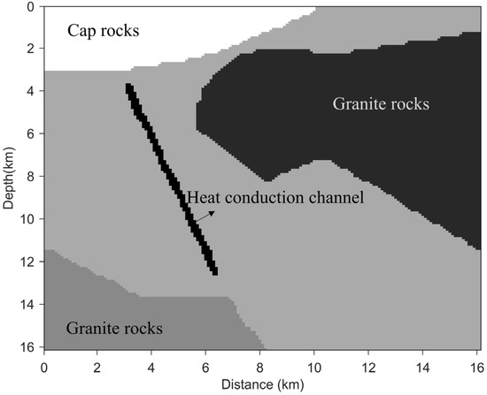
Figure 13.
Complex deep geological model of Gonghe Basin.
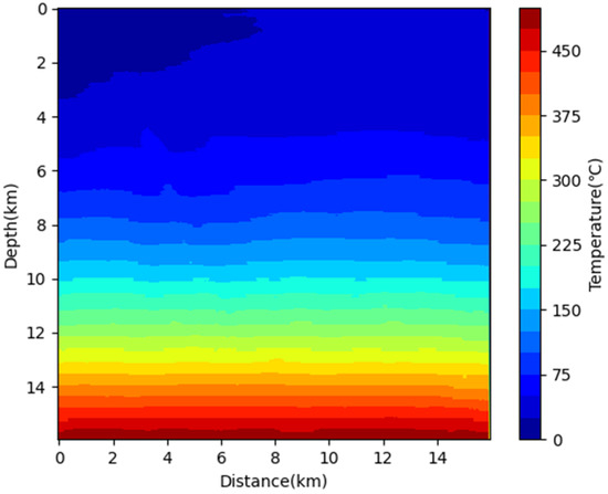
Figure 14.
Temperature field of complex model simulated from HDRT–UNet.
4. Discussion
The simulation results demonstrate that our proposed HDRT–UNet presents promising capabilities of simulating the temperature field of hot dry rocks. The purpose of this research was to use the HDRT–UNet to simulate the temperature field, to solve the problem of complicated setting conditions of the temperature field simulation and to achieve the results in a faster time. Although the temperature field simulated by our method is encouraging, many factors in the HDRT–UNet can affect its performance, including the size of the training data set, the setting of hyper–parameters (initial learning rate setting, batch size and loss function selection) and the structure of the neural network. Consequently, this section will discuss the advantages and disadvantages of the new method.
The limitation of our approach was that the simulation ability of the network predominantly depended on the data set. In general, the training data set should contain the rock parameters and structural characteristics of the 2D geological model to be predicted. That is, the supervised learning network used for the prediction has a direct impact on the selection of training data sets and the amount of data. Figure 15 shows the prediction result of the HDRT–UNet of the geological model of Figure 9 when there were no heat conduction channels in the data set. Figure 15 shows that there were obvious errors in the results of temperature field simulation, because the HDRT–UNet had not learned the parameters and structural characteristics of the heat conduction channels, and it was under–fitting when using the HDRT–UNet to simulate the temperature field. In most cases, a large number of large–scale and varied training samples will make the HDRT–UNet more powerful, but the training process takes longer.
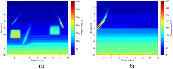
Figure 15.
Temperature field simulated from HDRT–UNet (excluding the heat conduction channels). (a) temperature field of model a simulated from HDRT–UNet; (b) temperature field of model b simulated from HDRT–UNet.
The advantage of our method is realizing an end–to–end simulation and reducing the influence of human factors. After a training process, the temperature field simulation result of complex models also met the experimental requirements, and the time consumption was shorter. The traditional finite element method used to simulate the temperature field of hot dry rock must include six modules: model establishment, parameter setting, boundary and initial conditions of the computing model, grid division, research and solution and post–processing, which not only requires manual operation, but also consumes more time. Neural network simulation of a temperature field only needs two steps: model establishment and network simulation, which greatly reduces manual operation and saves time. Table 2 shows the time taken using the finite element method to simulate the temperature field (including only the method solution process) and using HDRT–UNet to simulate the temperature field. The HDRT–UNet consumed less time, had a higher efficiency, and its accuracy was within an allowable error range.
Table 2.
Time used to simulate temperature sites.
5. Conclusions
A HDRT–UNet was proposed in this paper for simulating the temperature field of a complex deep HDR formation that provides an alternative to the finite element method. The conclusions are listed as follows:
- The simulation of the temperature field needs to deal with the relationship between thermal conductivity, specific heat capacity and density. We used the temperature field equation and thermal diffusivity equation to transfer the three parameters into the network to simulate the temperature field, thus realizing the fusion of multiple parameters into the network training.
- As a machine–learning method, our proposed method relies on training data sets and labels, which are simulated by the finite element method (FEM). The results of several numerical simulations demonstrate the feasibility of our proposed HDRT–UNet method in temperature field simulation and its better effect on the complex HDR model.
- Temperature simulation of several numerical HDR geological models by our HDRT–UNet method reached some conclusions. The cover layer had a great influence on the regional temperature field, and its low thermal conductivity lead to the temperature field above the cover layer being smaller than the surrounding temperature field. The thermal channel is the transportation channel with the temperature moving up. The transportation speed of heat energy in the thermal channel was obviously higher than that in the granite and crust, and the temperature in the thermal channel was also higher than that in the surrounding strata. However, granite showed the characteristics that the internal temperature field was higher than the surrounding geothermal field, and the heat energy migration speed was faster than the surrounding strata.
Author Contributions
Conceptualization, J.Z. and S.P.; methodology, W.G. and J.Z.; software, W.G.; formal analysis, W.G. and J.Z.; writing and editing, W.G. and J.Z. All authors have read and agreed to the published version of the manuscript.
Funding
This research is supported by the National Key Research and Development Program of China (grant no. 2020YFE0201300), and Fundamental Research Funds for the Central Universities (grant nos. 2021JCCXMT0 and 2602020RC130).
Institutional Review Board Statement
Not applicable.
Informed Consent Statement
Informed consent was obtained from all subjects involved in the study.
Data Availability Statement
Not applicable.
Acknowledgments
We thank Peng Research Group in CUMTB for support of this work. We thank Chen, Sheng, Hu and Wang in CUMTB for support of this work.
Conflicts of Interest
The authors declare no conflict of interest.
References
- Song, X.; Yu, S.; Li, G.; Yang, R.; Wang, G.; Zheng, R.; Li, J.; Lyu, Z. Numerical simulation of heat extraction performance in enhanced geothermal system with multilateral wells. Appl. Energy 2018, 218, 325–337. [Google Scholar] [CrossRef]
- Younas, U.; Khan, B.; Ali, S.M.; Arshad, C.M.; Farid, U.; Zeb, K.; Rehman, F.; Mehmood, Y.; Vaccaro, A. Pakistan geothermal renewable energy potential for electric power generation: A survey. Renew. Sustain. Energy Rev. 2016, 63, 398–413. [Google Scholar] [CrossRef]
- Zhang, C.; Huang, R.; Qin, S.; Hu, S.; Zhang, S.; Li, S.; Zhang, L.; Wang, Z. The high–temperature geothermal resources in the Gonghe−Guide area, northeast Tibetan plateau: A comprehensive review. Geothermics 2021, 97, 102264. [Google Scholar] [CrossRef]
- Bassam, A.; Santoyo, E.; Andaverde, J.; Hernández, J.A.; Espinoza–Ojeda, O.M. Estimation of static formation temperatures in geothermal wells by using an artificial neural network approach. Comput. Geosci. 2010, 36, 1191–1199. [Google Scholar] [CrossRef]
- Franco, A.; Vaccaro, M. Numerical simulation of geothermal reservoirs for the sustainable design of energy plants: A review. Renew. Sustain. Energy Rev. 2014, 30, 987–1002. [Google Scholar] [CrossRef]
- Li, M.; Lai, A. Review of analytical models for heat transfer by vertical ground heat exchangers (GHEs): A perspective of time and space scales. Appl. Energy 2015, 151, 178–191. [Google Scholar] [CrossRef]
- Blöcher, M.G.; Zimmermann, G.; Moeck, I.; Brandt, W.; Hassanzadegan, A.; Magri, F. 3D numerical modeling of hydrothermal processes during the lifetime of a deep geothermal reservoir. Geofluids 2010, 10, 406–421. [Google Scholar] [CrossRef]
- Zeng, Y.C.; Wu, N.Y.; Su, Z.; Wang, X.X.; Hu, J. Numerical simulation of heat production potential from hot dry rock by water circulating through a novel single vertical fracture at Desert Peak geothermal field. Energy 2013, 63, 268–282. [Google Scholar] [CrossRef]
- Shi, Y.; Song, X.; Li, G.; Yang, R.; Shen, Z.; Lyu, Z. Numerical investigation on the reservoir heat production capacity of a downhole heat exchanger geothermal system. Geothermics 2018, 72, 163–169. [Google Scholar] [CrossRef]
- Zhang, Y.; He, Z.; Qu, F.; He, D.; Hao, H.; Jiang, H. Numerical simulation of geothermal energy from dry hot rocks with gravity heat pipe. IOP Conf. Ser. Earth Environ. Sci. 2021, 647, 012124. [Google Scholar] [CrossRef]
- Feng, Z.J.; Zhao, Y.S.; Zhou, A.C.; Zhang, N. Development program of hot dry rock geothermal resource in the Yangbajing basin of China, Renew. Energy 2012, 39, 490–495. [Google Scholar]
- Zhao, J.B.; Song, H.D.; Li, D.; Zhang, Z. Research on Water Temperature Change of Hot Dry Rock Fracture Storage Layer in Shenyang. Appl. Mech. Mater. 2014, 580, 349–354. [Google Scholar] [CrossRef]
- Wei, X.; Feng, Z.J.; Zhao, Y.S. Numerical simulation of thermo–hydro–mechanical coupling effect in mining fault–mode hot dry rock geothermal energy. Renew. Energy 2019, 139, 120–135. [Google Scholar] [CrossRef]
- Zeng, Y.; He, B.; Tang, L.; Wu, N.; Song, J.; Zhao, Z. Numerical simulation of temperature field and pressure field of the fracture system at Zhangzhou geothermal field. Environ. Earth Sci. 2020, 79, 262. [Google Scholar] [CrossRef]
- Li, B.; Zhang, J.; Yan, H.; Zhou, N.; Li, M.; Liu, H. Numerical investigation into the effects of geologic layering on energy performances of thermal energy storage in underground mines. Geothermics 2022, 102, 102403. [Google Scholar] [CrossRef]
- Chen, P.; Sun, J.; Lin, C.; Zhou, W. Application of the finite volume method for geomechanics calculation and analysis on temperature dependent poromechanical stress and displacement fields in enhanced geothermal system. Geothermics 2021, 95, 0375–6505. [Google Scholar] [CrossRef]
- Üner, S.; Dogan, D.D. An integrated geophysical, hydrological, thermal approach to finite volume modelling of fault–controlled geothermal fluid circulation in Gediz Graben. Geothermics 2020, 90, 102004. [Google Scholar] [CrossRef]
- Li, T.; Han, D.; Yang, F.; Li, J.; Wang, D.; Yu, B.; Wei, J. Modeling study of the thermal–hydraulic–mechanical coupling process for EGS based on the framework of EDFM and XFEM. Geothermics 2021, 89, 101953. [Google Scholar] [CrossRef]
- Viesi, D.; Galgaro, A.; Santa, G.D.; di Sipio, E.; Garbari, T.; Visintainer, P.; Zanetti, A.; Sassi, R.; Crema, L. Combining geological surveys, sizing tools and 3D multiphysics in designing a low temperature district heating with integrated ground source heat pumps. Geothermics 2022, 101, 102381. [Google Scholar] [CrossRef]
- Tschannen, V.; Ettrich, N.; Delescluse, M.; Keuper, J. Detection of point scatterers using diffraction imaging and deep learning. Geophys. Prospect. 2020, 68, 830–844. [Google Scholar] [CrossRef]
- Gang, W.; Wang, J.; Wang, S. Performance analysis of hybrid ground source heat pump systems based on ANN predictive control. Appl. Energy 2014, 136, 1138–1144. [Google Scholar] [CrossRef]
- Rezvanbehbahani, S.; Stearns, L.A.; Kadivar, A.; Walker, J.D.; van der Veen, C.J. Predicting the Geothermal Heat Flux in Greenland: A Machine Learning Approach. Geophys. Res. Lett. 2017, 44, 12–271. [Google Scholar] [CrossRef]
- Haklidir, F.; Haklidir, M. Prediction of Reservoir Temperatures Using Hydrogeochemical Data, Western Anatolia Geothermal Systems (Turkey): A Machine Learning Approach. Nat. Resour. Res. 2019, 29, 2333–2346. [Google Scholar] [CrossRef]
- Maryadi, M.; Bramanthyo, P.; Zarkasyi, A.; Mizunaga, H. Estimation of near–surface temperature in Suwawa Geothermal Prospect, Gorontalo, Sulawesi, Indonesia, based on magnetotelluric and artificial neural network. IOP Conf. Ser. Earth Environ. Sci. 2021, 851, 012018. [Google Scholar] [CrossRef]
- Vivas, C.; Salehi, S. Real–Time Model for Thermal Conductivity Prediction in Geothermal Wells Using Surface Drilling Data: A Machine Learning Approach. In Proceedings of the 46th Workshop on Geothermal Reservoir Engineering Standford University, Standford, CA, USA, 15–17 February 2021. [Google Scholar]
- He, J.; Li, K.; Wang, X.; Gao, N.; Mao, X.; Jia, L. A Machine Learning Methodology for Predicting Geothermal Heat Flow in the Bohai Bay Basin, China. Nat. Resour. Res. 2022, 31, 237–260. [Google Scholar] [CrossRef]
- Yang, W.; Xiao, C.; Zhang, Z.; Liang, X. Identification of the formation temperature field of the southern Songliao Basin, China based on a deep belief network. Renew. Energy 2022, 182, 32–42. [Google Scholar] [CrossRef]
- Mahmoodpour, S.; Singh, M.; Bär, K.; Sass, I. Thermo–hydro–mechanical modeling of an enhanced geothermal system in a fractured reservoir using carbon dioxide as heat transmission fluid—A sensitivity investigation. Energy 2022, 254, 124266. [Google Scholar] [CrossRef]
- Mahmoodpour, S.; Singh, M.; Turan, A.; Bär, K.; Sass, I. Simulations and global sensitivity analysis of the thermo–hydraulic–mechanical processes in a fractured geothermal reservoir. Energy 2022, 247, 123511. [Google Scholar] [CrossRef]
- Ronneberger, O.; Fischer, P.; Brox, T. U–net: Convolutional Networks for Biomedical Image Segmentation. In Proceedings of the International Conference on Medical Image Computing and Computer–Assisted Intervention, Munich, Germany, 5–9 October 2015; Springer: Cham, Switzerland, 2015; pp. 234–241. [Google Scholar]
- Kingma, D.; Ba, J. Adam: A Method for Stochastic Optimization. arXiv 2014, arXiv:1412.6980. [Google Scholar] [CrossRef]
- Loshchilov, I.; Hutter, F. SGDR: Stochastic Gradient Descent with Warm Restarts. arXiv 2016, arXiv:1608.03983. [Google Scholar]
- Zhang, C.; Jiang, G.; Shi, Y.; Wang, Z.; Wang, Y.; Li, S.; Jia, X.; Hu, S. Terrestrial heat flow and crustal thermal structure of the Gonghe–Guide area, northeastern Qinghai–Tibetan plateau. Geothermics 2018, 72, 182–192. [Google Scholar] [CrossRef]
- Lu, C.; Lin, W.; Gan, H.; Liu, F.; Wang, G. Occurrence types and genesis models of hot dry rock resources in China. Environ. Earth Sci. 2017, 76, 646. [Google Scholar] [CrossRef]
- Wang, B.; Li, B.X.; Ma, X.H. The prediction of the depth and temperature of the reservoir in the evaluation of hot dry rock (HDR) for Gonghe–Guide basin. Ground Water 2015, 37, 28–31. [Google Scholar]
- Ren, H.D.; Wang, T.; Zhang, L.; Wang, X.X.; Huang, H.; Feng, C.Y.; Teschner, C.; Song, P. Ages, sources and tectonic settings of the Triassic igneous rocks in the easternmost segment of the East Kunlun Orogen, central China. Acta Geol. Sin. 2016, 90, 641–668. [Google Scholar]
- Gao, J.; Zhang, H.; Zhang, S.; Chen, X.; Cheng, Z.; Jia, X.; Li, S.; Fu, L.; Gao, L.; Xin, H. Three–dimensional magnetotelluric imaging of the geothermal system beneath the Gonghe Basin, Northeast Tibetan Plateau. Geothermics 2018, 76, 15–25. [Google Scholar] [CrossRef]
Publisher’s Note: MDPI stays neutral with regard to jurisdictional claims in published maps and institutional affiliations. |
© 2022 by the authors. Licensee MDPI, Basel, Switzerland. This article is an open access article distributed under the terms and conditions of the Creative Commons Attribution (CC BY) license (https://creativecommons.org/licenses/by/4.0/).