Solar Irradiance Nowcasting System Trial and Evaluation for Islanded Microgrid Control Purposes

Abstract

The rapid increase in solar photovoltaic (PV) integration into electricity networks introduces technical challenges due to varying PV outputs. Rapid ramp events due to cloud movements are of particular concern for the operation of remote islanded microgrids (IMGs) with high solar PV penetration. PV systems and optionally controllable distributed energy resources (DERs) in IMGs can be operated in an optimised way based on nowcasting (forecasting up to 60 min ahead). This study aims to evaluate the performance under Perth, Western Australian conditions, of an all-sky imager (ASI)-based nowcasting system, installed at Murdoch University in Perth, Western Australia (WA). Nowcast direct normal irradiance (DNI) and global horizontal irradiance (GHI) are inputted into a 5 kWp solar PV system with a direct current (DC) power rating/alternating current (AC) power rating ratio of 1.0. A newly developed classification method provided a simplified irradiance variability classification. The obtained nowcasting system evaluation results show that the nowcasting system’s accuracy decreases with an increase in lead time (LT). Additionally, the nowcasting system’s accuracy is higher when the weather is either mostly clear (with a recorded LT15 mean absolute deviation (MAD) of 0.38 kW) or overcast (with a recorded LT15 MAD of 0.19 kW) than when the weather is intermittently cloudy with varying cloud conditions (with a recorded LT15 MAD of 0.44 kW). With lower errors observed in lower LTs, overall, it might be possible to integrate the nowcasting system into the design of IMG controllers. The overall performance of the nowcasting system at Murdoch University was as expected as it is comparable to the previous evaluations in five other different sites, namely, PSA, La Africana, Evora, Oldenburg, and Julich.

1. Introduction

Background and Motivation

The most significant challenge that the world is currently facing is anthropogenic climate change, thus driving the development of sustainable energy solutions to avoid the use of fossil fuels. This has led to the increasing utilisation of renewable energy resources mostly solar photovoltaic, wind, and hydro. However, solar photovoltaic (PV) power can have short-term variability, mostly due to variable cloud cover which presents challenges to increasing PV penetration levels, particularly in islanded microgrids (IMGs) [1].

Currently, in some IMGs, these fluctuations in PV power output are being managed by limiting PV connections, curtailing PV power output, using battery storage systems to compensate for fluctuations in PV power output, or by using dump loads, flywheels, or fuel cells [2,3,4,5]. Limiting power ramp (power ramp limiting is limiting/minimising the fluctuation rate of PV output when the irradiance is fluctuating but still delivering maximum available power) is another technique to control the variable renewable energy generation systems’ output power [6].

However, these currently employed solutions can be costly and may limit renewable energy resources’ penetration [7]. Therefore, utilities are investigating and trialling new technologies and control methods (e.g., nowcasting) to meet the customers’ desire to enable more rooftop PV within IMGs [8].

Nowcasting, which is very short-term solar irradiance forecasting, can possibly assist in mitigating irradiance variability impacts on system management by predicting a near-future PV output, which can be integrated into the control of IMGs, resulting in the provision of the operational/spinning reserve to cover for the predicted reduction in PV output. Operational reserve strategies incorporating nowcasting can provide benefits such as reduced fuel consumption and increased hosting capacity [8]. Additionally, nowcasting may reduce the required battery energy storage systems, thus reducing the system’s capital cost [9]. In the analysis by Harris [9], it is reported that the battery energy storage system would have been doubled in the absence of a nowcasting system. Nowcasting may also be integrated for ramp rate control during cloud events by curtailing PV output.

All-sky imagers (ASIs) (All sky imagers are sky-facing surveillance cameras used to take images of the sky at certain set time intervals) can be used for the development of nowcasting systems for irradiance forecasts. The process in which nowcasts are performed using ASIs is explained in detail by [10,11,12,13,14,15,16,17]. A few nowcasting tools have been developed and/or evaluated under different conditions around the world.

Table 1. Nowcasting tool examples.

Product/System and Manufacturer	Forecast Parameters	Forecast Horizon	Application Examples and References
Q4cast by CSP Service (Almeria, Spain)	Global horizontal irradiance (GHI), direct normal irradiance (DNI) and global tilted irradiance (GTI)	15 min	Operational at two solar research centres and a commercial 50 MW solar power plant, La Africana in Spain [22].
Steady Eye by Steadysun (Le Bourget-du-Lac, France)	GHI, DNI, GTI, PV system output (percentiles)	Up to 60 min, updated every minute	Hybrid system [21].
InstaCast by Reuniwatt (Sainte-Clotilde, La Réunion, France)	GHI, DNI, GTI, PV system output	30 min	Microgrid Example, Brazil [23].
SkyInsight by Reuniwatt	GHI, DNI, GTI, PV system output	10 min	Hybrid PV-Diesel system [20].
CloudCAM by Fulcrum3D (Artarmon, NSW, Australia)	Irradiance/solar power output	Up to 15 min (depends on local atmospheric conditions)	Karratha Airport 1MW Solar Project [9].

summarises the available sky-imagery-based nowcasting tools suitable for system-level control applications [18]. However, the product information and information on the application experiences of some outlined tools in Table 1 is limited (especially for InstaCast and SkyInsight by Reuniwatt and Steady Eye by Steadysun) as they are primarily based only on the manufacturer-provided information [19,20,21]. Reuniwatt analysed the benefits of integrating nowcasting in a hybrid PV/diesel system. Results of this study by Boudreault et al. [20], suggest that the integration of nowcasting to the hybrid PV/diesel system reduces the system’s fuel consumption and reduces potential blackouts.

The nowcasting system is of interest in Western Australia due to the existence of many remote IMGs with abundant solar resources. The utilities and industries operating IMGs are interested to examine the possibility of integrating nowcasting in the control of IMGs, which can potentially lead to increased PV penetration [8]. One of the readily available ASI nowcasting tools, developed by the DLR Institute of Solar Research is installed and evaluated at Murdoch University in Perth, Western Australia (WA) [22,24]. The purpose of trialling the nowcasting system is to determine its accuracy in predicting near-future solar PV power output in Perth conditions.

The performance of this ASI nowcasting system has been evaluated in Germany (Oldenburg and Julich), Portugal (Evora), and Spain (La Africana and PSA) [25]. In the performance evaluation, the mean absolute deviation (MAD) and root mean square deviation (RMSD) were calculated for DNI, and in some locations also for GHI, but not for solar PV power output. However, this study focuses on the prediction of PV power output and related uncertainties due to cloud events. The nowcast PV output power and ultimately the error in the prediction is relevant for the IMG operators for accurate dispatching and ramp rate control.

The following are outlined as the contributions of this study:

• DNI variability classification is one of the processes involved in the nowcasting system performance evaluation [25]. The variability indices by [25,26,27,28,29,30] were used in the study by Nouri et al. [25] to determine eight DNI variability classes. The persistence model has been reported in the literature to be highly accurate on cloudless days and highly overcast days with almost constant cloud conditions but incurs huge errors during intermittently cloudy conditions [27]. Against this backdrop, and because most days evaluated in this study are intermittently cloudy, a new simplified classification model is developed. This model classifies conditions into mostly clear sky, intermittently cloudy, and overcast. This simplified approach is deemed suitable in view of the application of nowcasting in IMG control where the distinction between mostly clear sky, overcast, and intermittently cloudy conditions may align well with distinct control regimes suitable for these conditions. The proposed method utilises the mean and standard deviation (STD) of daily DNI and GHI datasets, as well as integration tools for the classification.
• This study evaluates the performance of the nowcasting system in the southern hemisphere (Perth, Western Australia). The performance of the nowcasting system has been evaluated in northern hemisphere locations in Germany (Oldenburg and Julich), Portugal (Evora), and Spain (La Africana and PSA) [25].
• In the DigSILENT PowerFactory (PF), the highest resolution that can be inputted using the inbuilt characteristic tool is 1 min. In this study, higher resolution (30 s) irradiance data are utilised for the DNI and GHI nowcasts. These nowcasts are then inputted into the solar PV system in PF for nowcast PV power output determination. As a contribution, a scripting program was developed to input these high-resolution DNI and GHI data into the solar PV system in PF to be able to determine the PV power output, the MAD, and the RMSD of the PV power output.

This paper is structured into five sections. Section 2 describes an overview of the nowcasting system set up at Murdoch University in Perth, followed by the performance evaluation in Section 3. The results are presented and discussed in Section 4, and finally, the conclusions and recommendations for future work are presented in Section 5 of this paper.

2. An Overview of the Used Nowcasting System Set-Up

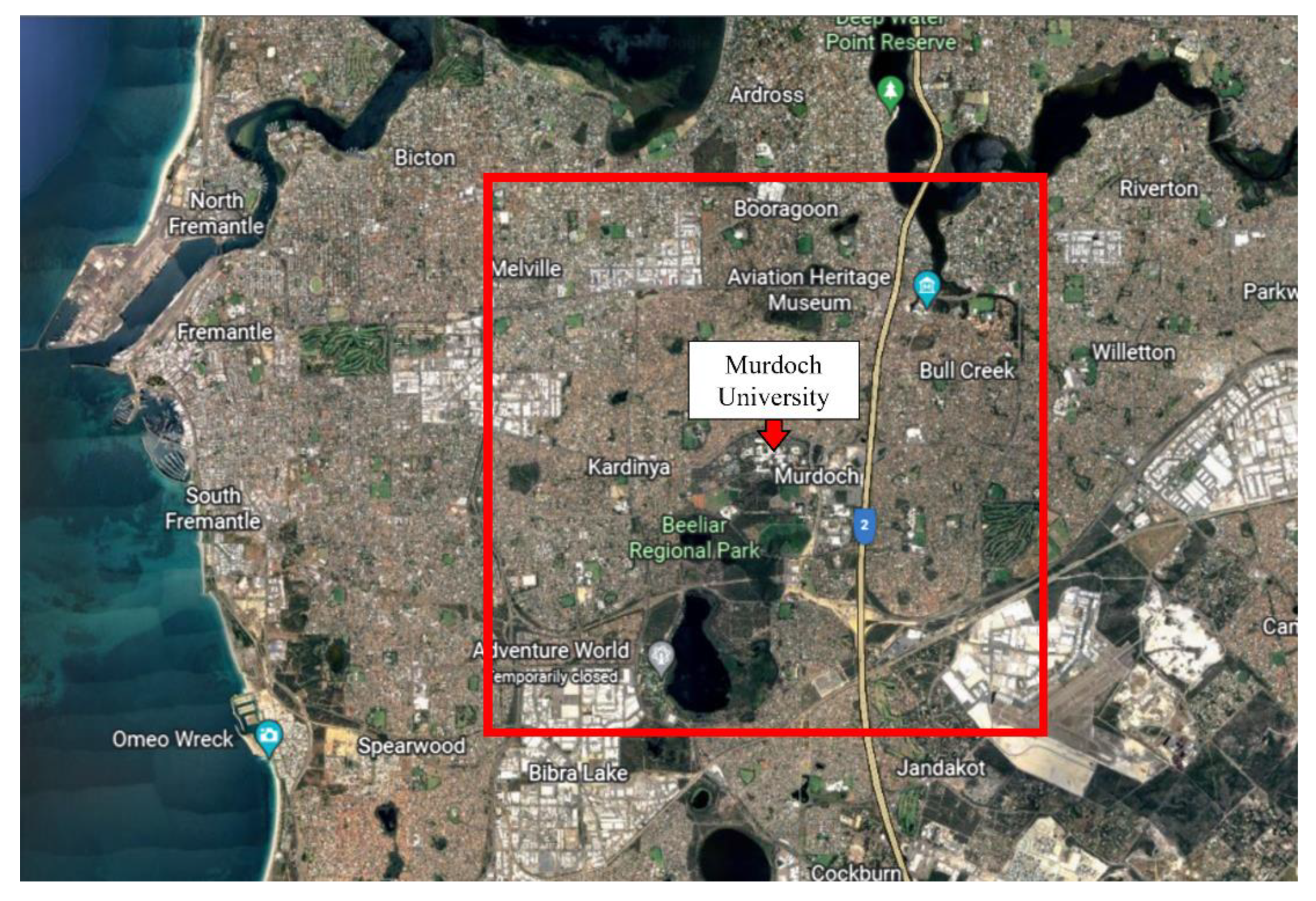
Two MOBOTIX Q26, 6 megapixels (MP), fisheye lens surveillance cameras are utilized as ASIs at Murdoch University, Perth Campus in Western Australia.

Table 2. Nowcasting system components and locations.

System Component	Sensitivity (µV/W/m²)	Response Time (s)	Field of View (°)	Operational Temperature Range (°C)	Location at Murdoch University	Longitude (° East)	Latitude (° South)	Altitude (m)
ASI 1			180		Renewable Outdoor Test Area (ROTA)	115.84051	32.07048	27
ASI 2			180		Engineering and Energy Building 220 (Bld 220)	115.8371	32.06613	52
CHP1 Pyrheliometer	7 to 14	<5	5 ± 0.2	−40 to +80	(Bld 220)	115.8371	32.06613	52
2 × CM 11 Pyranometers	7 to 14	<5	180	−40 to +80	(Bld 220)	115.8371	32.06613	52
Thermofisher DT80 Datalogger					(Bld 220)	115.8371	32.06613	39
Sky server					(Bld 220)	115.8371	32.06613	39
Murdoch University weather station					Murdoch University	115.8389	32.06732	6

presents the technical details of the measurement equipment [31,32] and location details of the ASIs, which are mounted 640 m apart from each other and other nowcasting system components. The fisheye lenses of the cameras produce 180° × 180° hemispherical images encapsulating the viewable sky from the camera location. Set to the maximum image format of 6 megapixels (3072 × 2048), the cameras capture images every 30 s.

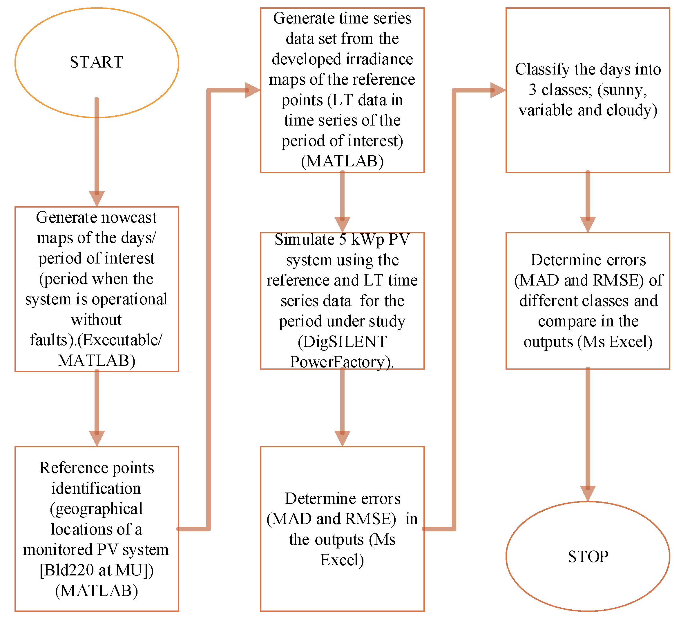
A ground-based meteorological station at Murdoch University also forms part of the nowcasting system. The flow diagram in Figure 1 summarises the configuration and processing chain, whilst

Table 3. ASI nowcasting system processing steps [8].

Step	Description
1	Cloud segmentation [22,33,34].
2	Cloud height and 3D cloud coordinates ‘determination [35].
3	Cloud motion vectors extraction [35].
4	Future cloud position prediction [36].
5	Cloud transmittance properties ’measurements [37].
6	Cloud shadows determination [36].
7	Derivation of DNI and GHI maps [36].

summarises the steps involved in the processing chain of the nowcasting system applied in this study. Figure 2a,b shows a MOBOTIX Q26 ASI mounted at Murdoch University and an example of a sky image taken by the ASI, respectively.

For evaluating nowcasts, high-resolution solar irradiance data are required. At least one DNI measurement sensor needs to be installed adjacent to one of the ASIs for evaluation purposes. In this study, a Kipp and Zonen CHP1 pyrheliometer used for DNI measurements is installed on a Kipp and Zonen SOLYS2 sun tracker which is mounted less than one meter from the ASI 2. In addition to the DNI, the diffuse horizontal irradiance (DHI) and GHI are also recorded. Kipp and Zonen CM11 pyranometers are used for this purpose. A DT80 Series 2 data logger is used to sample and record the irradiance and temperature measurements from the pyranometers and pyrheliometer.

Network, Connectivity and Storage

The ASI system at Murdoch University comprises two ASIs and a datalogger connected via ethernet on a local area network. The sky images and irradiance measurements are stored via the FTP to a server. The Mobotix cameras are both hardwired for power via a power over ethernet power supply, whilst the data logger and the SOLYS2 are hardwired with a regulated 24 V DC supply. The maintenance of the cameras and irradiance sensors is carried out periodically with a set schedule and maintenance log kept for consistency and fault finding. Figure 3a,b shows the complete setup at the Murdoch University location. The geographical coordinates of these components are presented in Table 2.

3. Nowcasting System Performance Evaluation

The methodology for the performance evaluation of the ASI nowcasting system considering various atmospheric conditions is outlined in this section. In stable conditions with fewer fluctuations in DNI (low temporal irradiance variability), uncertainties decrease, and when DNI variability is high (high temporal irradiance variability), uncertainties also increase [38], thus low or high metric errors are detected depending on the dataset selected.

Figure 4 summarises the methodology employed for the performance evaluation of the nowcasting system. The ASI nowcasting system is utilised to generate irradiance nowcast maps, up to 15 min ahead. A reference point (Building 220 at Murdoch University, where the irradiance sensors are located) was then identified from the generated maps. Time-series DNI and GHI datasets are then produced from the irradiance maps and used as inputs to a 5 kWp PV system in PF. The MAD and RMSD are then calculated from the output power from the PV system.

3.1. Generation of Nowcast Irradiance Maps

The first phase of the methodology included the utilisation of MATLAB for the generation of DNI and GHI maps, the identification of geographical locations of the irradiance sensors on top of Building 220 at Murdoch University, and the generation of lead time (LT) time-series DNI and GHI datasets from the generated maps. The LTs were determined for 15 min ahead in 1 min intervals, thus from LT1 to LT15, representing nowcasts from 1 min to 15 min ahead. The generated irradiance maps covered an area of 8 km by 8 km. The area covered by the generated irradiance maps is enclosed as shown in Figure 5, whilst the pictorial description of the nowcast is shown in Figure 6.

3.2. Simulation of PV System

A total of 47 days were considered for this study. These 47 days (between January 2021 and October 2021) represent all seasons and weather conditions. Furthermore, they denote the days when the nowcasting system was fully operational, recording all the datasets required for the nowcasts.

The GHI and DNI time-series data of those days were generated from LT0 (which is the same as the recorded reference data) to LT15. The generated LT0 to LT15 time-series DNI and GHI time-series data are fed as inputs to a 5 kWp PV system, with a direct current (DC)/alternating current (AC) ratio of 1.0, in the ‘Solar Calculation Model’ in PF through DPL scripting. The ‘Solar Calculation Model’ is selected to be able to feed into a high resolution (<1 min) irradiance dataset for the solar PV model. Power in kW is generated as one of the output parameters, which is then used to determine the nowcast errors.

3.3. Error Metrics

The discretised $RMS{D}_C$ and $MA{D}_C$ for both of the PV system output over the lead times are determined using Equations (1) and (2). The $RMS{D}_C$ is an accuracy measure. In general, a lower $RMS{D}_C$ is better since the lower the $RMS{D}_C$, the higher the accuracy of the nowcasting system. The $MA{D}_C$ is the average distance between each data point and the mean which outlines the variability in a dataset.

$$MA{D}_C=\frac{1}{n_C}{{\displaystyle \sum }}_{i_c=1}^{n_C}\left|Y_{i_c}-{\widehat{Y}}_{i_c}\right|$$

(1)

$$RMS{D}_C={\left[\frac{1}{n_C}{{\displaystyle \sum }}_{i_c=1}^{n_C}{\left(Y_{i_c}-{\widehat{Y}}_{i_c}\right)}^2\right]}^{\frac{1}{2}}$$

(2)

where $Y_{i_c}$ and ${\widehat{Y}}_{i_c}$ represent the reference and the corresponding nowcasted output power value from the simulations, respectively. The reference output power is power generated using reference DNI and GHI data, while the nowcast DNI and GHI generated nowcast output power. The number of used validation time stamps is denoted by $n_C$, whilst $i_c$ identifies all timestamps belonging to the same output power variability class. Further analysis of errors after the classification of the days under consideration was performed.

3.4. DNI and GHI Variability Classification

Three classes are formulated for the DNI variability as displayed in

Table 4. DNI and GHI variability classification.

Class	Description
1	Mostly clear sky conditions with low temporal irradiance variability.
2	Intermittently cloudy with high temporal irradiance variability.
3	Overcast with low temporal irradiance variability.

together with corresponding brief descriptions. The three classes are mostly clear sky, intermittently cloudy, and overcast. During the mostly clear sky conditions, the DNI is expected to have a bell shape curve over a day, whereas, during the overcast conditions, the DNI is expected to vary between 0–500 W/m². As for the intermittently cloudy days, the DNI can fluctuate from a low to high irradiance value and also produce a bell shape curve. There are some days in which characteristics of all the three defined classes or more than one class may be observed, for example, a morning with mostly clear sky conditions, followed by noon with intermittently cloudy conditions and an overcast afternoon.

Figure 7a shows an example of a day in which all the three classes are observed on the same day, whilst Figure 7b displays the metrics used for the classification exercise. Figure 7c,d shows examples of the actual DNI characteristics of the three classes. The shaded areas in Figure 7a,b are the regions where the DNI values are expected to be present. Both the mostly clear sky and the overcast days have a small area compared to the intermittently cloudy day. This was used as the first metric in identifying the intermittently cloudy day. Another metric, the sliding hourly STD of the DNI values can be used to identify the rest of the days. A high STD shows that the DNI values are far from the mean value, while a low STD shows that the DNI values are close to the mean. The days on which multiple classes are observed are also determined by calculating sliding hourly STD and area within the day and then classified on an hourly period using the metrics shown in Table 4. The overall class of the entire day is then determined by the class with the highest frequency observed within the day.

3.4.1. Assigning High and Low Values to Metrics

The proposed method requires initial values of the classification metrics, the STD and shaded area, to determine whether the metrics of a particular day fall into the high or low class. The averages of the STD and the shaded area are stored as initial conditions within the program.

3.4.2. Determining High and Low STD

A mostly clear sky day and an overcast day are manually selected by scanning the sky images at the beginning. Sliding STDs of each day are computed on an hourly basis to allow for intraday variabilities. An average of the two days’ STDs is then computed and stored as an initial condition. If a random hour on a random day is selected and its STD is computed, a comparison of this newly computed STD to the initial condition (average STD, ~170 W/m²) will determine whether that hour has a high (>initial condition) or low (<initial condition) STD. A mostly clear sky hour and an hour with variable DNI (intermittently cloudy) will both have high STDs, whilst an overcast hour will have a lower STD compared to the initial condition.

3.4.3. Determining High and Low Shaded Area

A mostly clear sky day and an overcast day are manually selected by scanning the sky images at the beginning, then followed by a calculation of their individual shaded areas using Equation (3), and then computing the average of the shaded areas. This average of the shaded areas is then stored as an initial condition (~1272 W/m²). If a random day is picked and its shaded area is calculated, a comparison of the calculated shaded area with the initial condition of the shaded area will determine whether the shaded area of that day falls in the high or low category. The shaded area is assigned a high value if it is greater than the initial condition and low if the calculated shaded area is less than the initial condition. A mostly clear sky and an overcast day will both have an area lower than the initial condition set, while an intermittently cloudy day will have an area higher than the initial condition set.

To find this shaded area, the difference between the first and second values of the DNI is calculated. This difference is then added to the difference between the second and third values of DNI. The sum of all the differences will give the shaded area of the class for that day. Equation (3) shows the shaded area formula utilised, where A is the shaded area of the class, n is the number of DNI datasets for that day, and x is the DNI data.

$$A={{\displaystyle \sum }}_{i=1}^n\left|x_i-x_{i+1}\right| i \le n$$

(3)

Table 5. (a) Conditions used for classification. (b) Dates chosen for initial conditions.

(a)
Class	Value of Shaded Area Compared to the Initial Condition	Value of STD Compared to the Initial Condition
Mostly clear sky	Low	High
Intermittently cloudy	High	High
Overcast	Low	Low
(b)
Weather Condition	Day Chosen
Mostly clear sky	5 January 2021
Overcast	10 June 2021

a summarises the conditions that can be used to identify the different classes. To classify a selected hour, if both the value of the shaded area and STD are high, with respect to the initial condition, the hour is classified as intermittently cloudy. If both assigned values are low, the hour is classified as overcast, otherwise, the selected hour would be classified as mostly clear sky. Table 5b shows the days used to calculate the initial conditions for the classification exercise.

3.4.4. Classification Examples

Three days, displayed in Figure 7c,d (5 June, 6 June, and 10 June), were chosen and classified using the newly developed classification method of this study. Hourly classifications are calculated over the day, and the class with the majority occurrences in a day is chosen to be the overall class of the day.

Table 6. Class Frequency for 3 specific days (See Figure 7c,d).

Date	Frequency Overcast	Frequency Intermittently Cloudy	Frequency Mostly Clear Sky	Chosen Class
5 June 2021	0	3	7	Mostly Clear Sky
6 June 2021	0	10	0	Intermittently Cloudy
10 June 2021	6	3	1	Overcast

shows the frequency of each class on an hourly basis for 10 h (from 07.00 to 17.00) and the chosen class for that day.

4. Results and Discussion

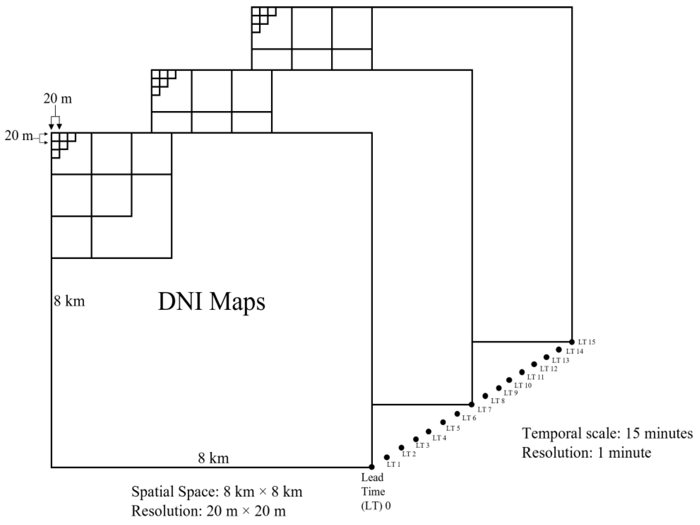
To evaluate the operation of the nowcasting system under Western Australian conditions, models were developed, and this section reports the outcomes of the analysis. Figure 8 is a three-dimensional virtual modelling space with cloud models and a topographical map around Perth with spatial DNI information generated at a 30 s resolution. This resolution corresponds to a 30 s resolution at which the sky images are logged as inputs for the generation of the irradiance maps. These maps cover a surface area of 64 km² (8 km × 8 km). The Z-axis in Figure 8 shows the cloud height at the location of the study. Cloud height is of importance as it determines how far into the future an irradiance forecast can be determined. 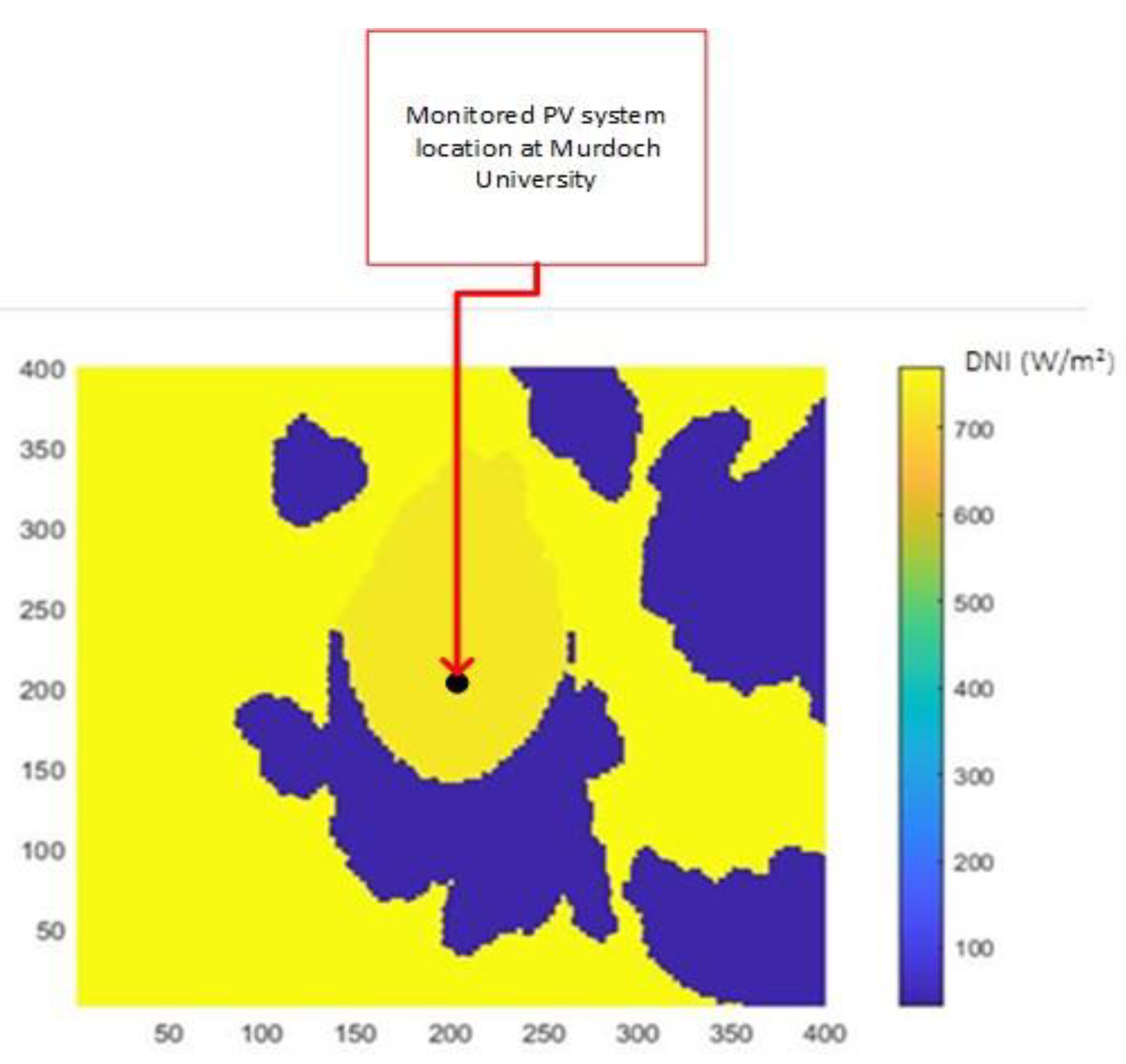Figure 9 is a two-dimensional exemplary nowcast DNI map also covering a surface area of 64 km². In two dimensions, these maps are displayed via 400 × 400 pixels, with each pixel representing certain geographical locations of 20 m × 20 m. From Figure 8, it is observed that at the instant when that DNI map was captured, the day was partly cloudy. The geographical location of the monitored PV system (Figure 9) on top of Building 220 is 32.06613° south, 115.8371° east.

Figure 10 shows a sample output from the simulation displaying the PV power in kW. It is observed that the output power is consistent with the input irradiance in the PF PV model. From Figure 10, it can also be seen that there is an increase, then a decrease in the output power as the day progresses, from 6 am to 6 pm. Additionally, Figure 10 displays sample PV power outputs due to LT0 (measured irradiance data at the time of the nowcast LT7 value) and due LT7 (nowcast of 7 min ahead). It is observed that days 1, 3, 4, and 5 are mostly clear sky days, whilst day 2 is intermittently cloudy. It is seen that the errors are minimum on mostly clear days to intermittently cloudy. This is denoted by the almost overlapping of power (LT0) and power (LT7) curves in mostly clear sky days as opposed to intermittently cloudy days. The overlapping of the plots shows the matching between the measured PV output power and the nowcast PV output power.

Table 7. Distribution of days under analysis.

Class	Number of Days
1 (mostly clear sky)	17
2 (Intermittently cloudy)	24
3 (Overcast)	6

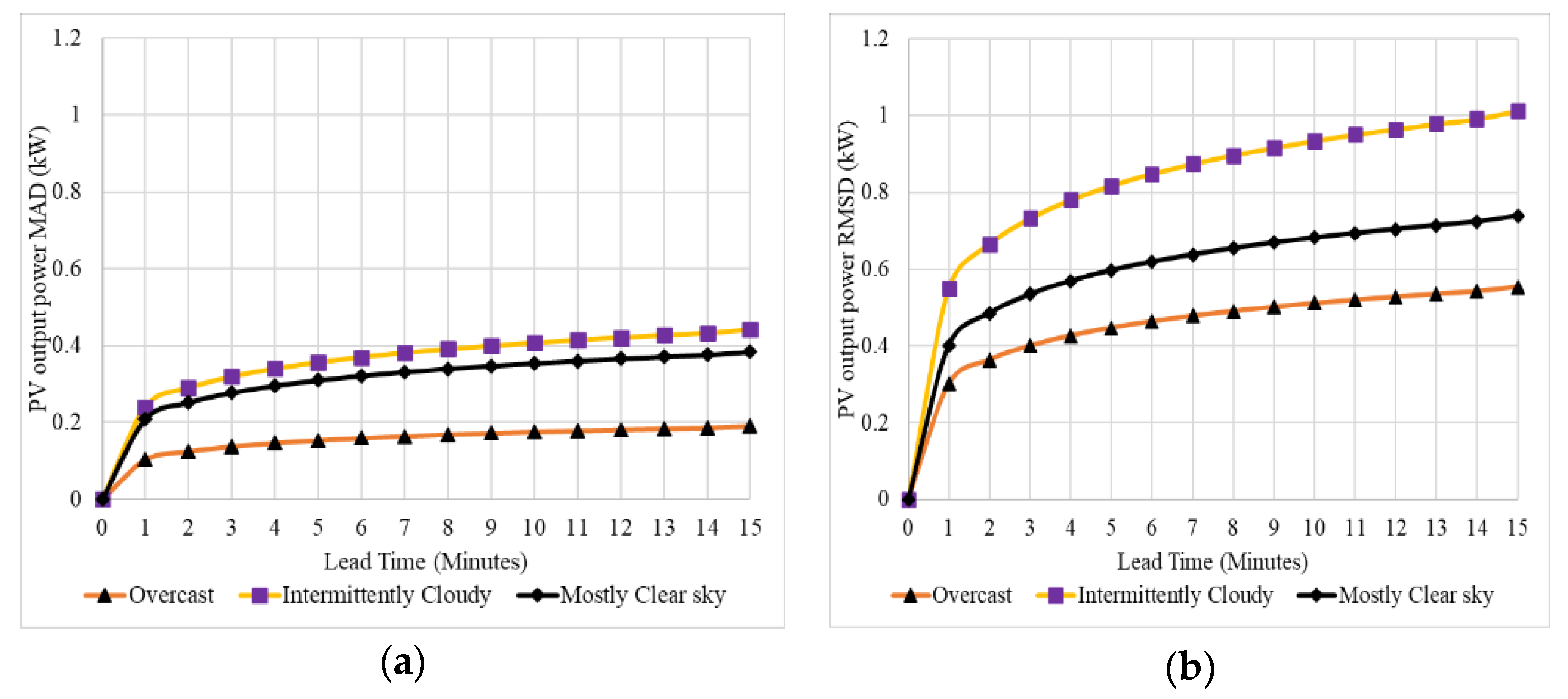
shows the distribution of the days under analysis. Figure 11a,b displays the 5 kWp PV system output power MADs and RMSDs, respectively. The lowest deviations are observed in class 1 (with an LT15 MAD of 0.38kW), which represents mostly clear sky conditions, and class 3 (with an LT15 MAD of 0.19kW), which represents overcast, whilst the highest deviations are observed for class 2 (with an LT15 MAD of 0.44 kW), which represents intermittently cloudy conditions.

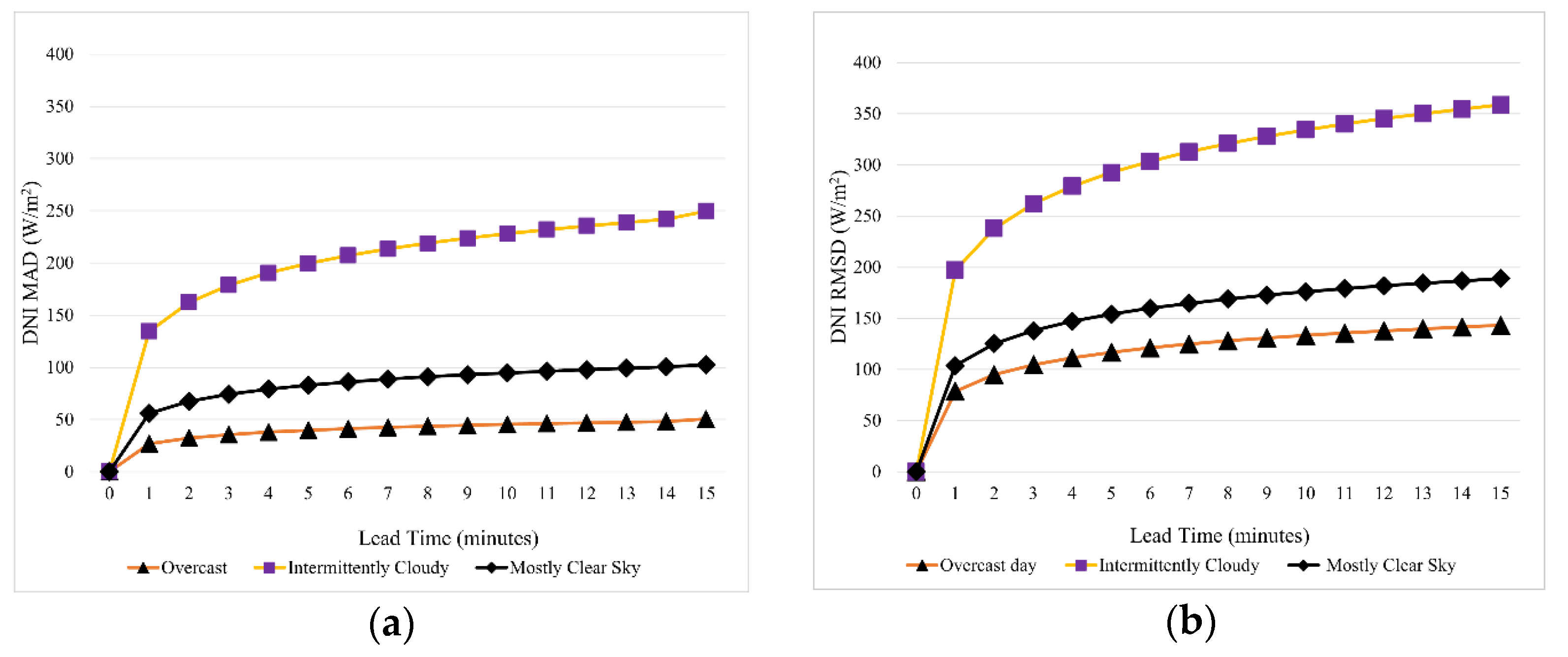
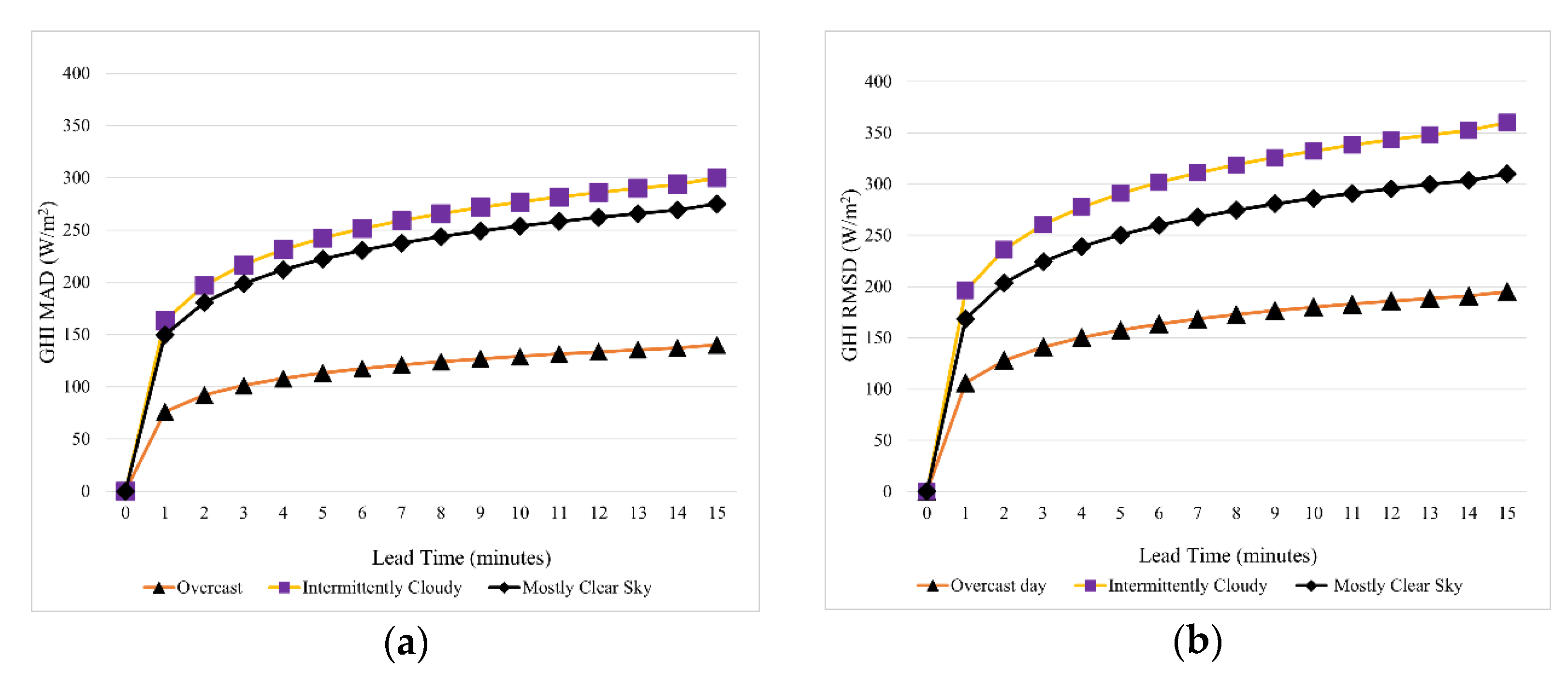
Figure 12 and Figure 13 display the DNI MADs, DNI RMSDs, GHI MADs, and GHI RMSDs, respectively, for the same time frame as that of Figure 11a,b, classified using the developed classification method in this study. The results displayed in Figure 12 and Figure 13 are consistent with those observed in Figure 11a,b. As displayed in Figure 12a, the lowest deviations are observed in class 3 (with an LT15 DNI MAD of 50 W/m²), which represents overcast and class 1 (with an LT15 DNI MAD of 102 W/m²), which represents mostly clear sky conditions whilst the highest deviations are observed for class 2 (with an LT15 DNI MAD of 250 W/m²), which represents intermittently cloudy conditions.

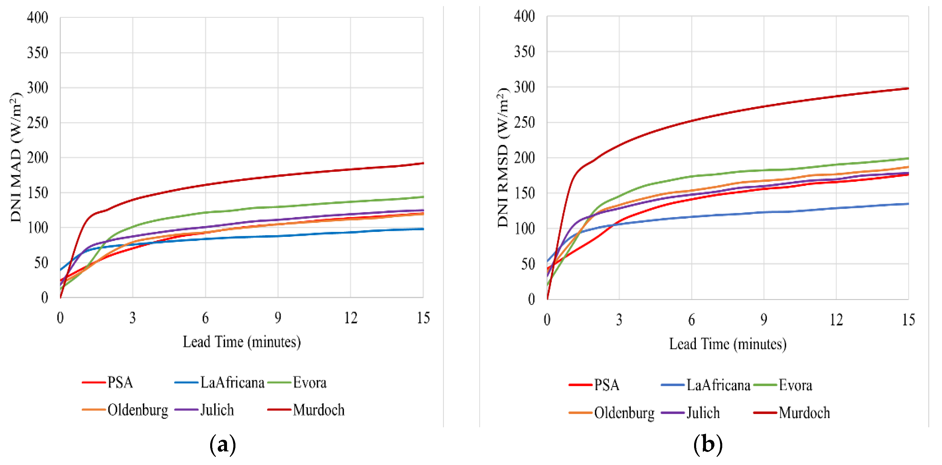
From Figure 14a, it is observed that the DNI MAD of the ASI system at Murdoch University is higher than the other five sites, and so is the DNI RMSD, as shown in Figure 14b. The differences between the DNI MAD and DNI RMSD values at LT15 for the Murdoch University ASI system to the highest DNI MAD and DNI RMSD values of the other five sites are around 48 W/m² and 99 W/m², respectively. These differences could be mainly due to the evaluation periods of each site. PSA and LaAfricana were evaluated over a year whilst Evora, Oldenburg Julich, and Murdoch University, were evaluated for only 42, 86, 80, and 47 days, respectively, during a certain period of the year. Additionally, the evaluation period for Evora was during the summer period where rainfall is at its lowest with a majority of mostly clear sky conditions, whilst for Oldenburg and Julich, the evaluation was during a heavy rainfall period where the sky is mostly overcast. On the contrary, as shown in Table 7, the ASI system at Murdoch University was evaluated over 47 days, with the majority of the days under evaluation falling under the intermittently cloudy class, which is associated with high errors due to high DNI variability.

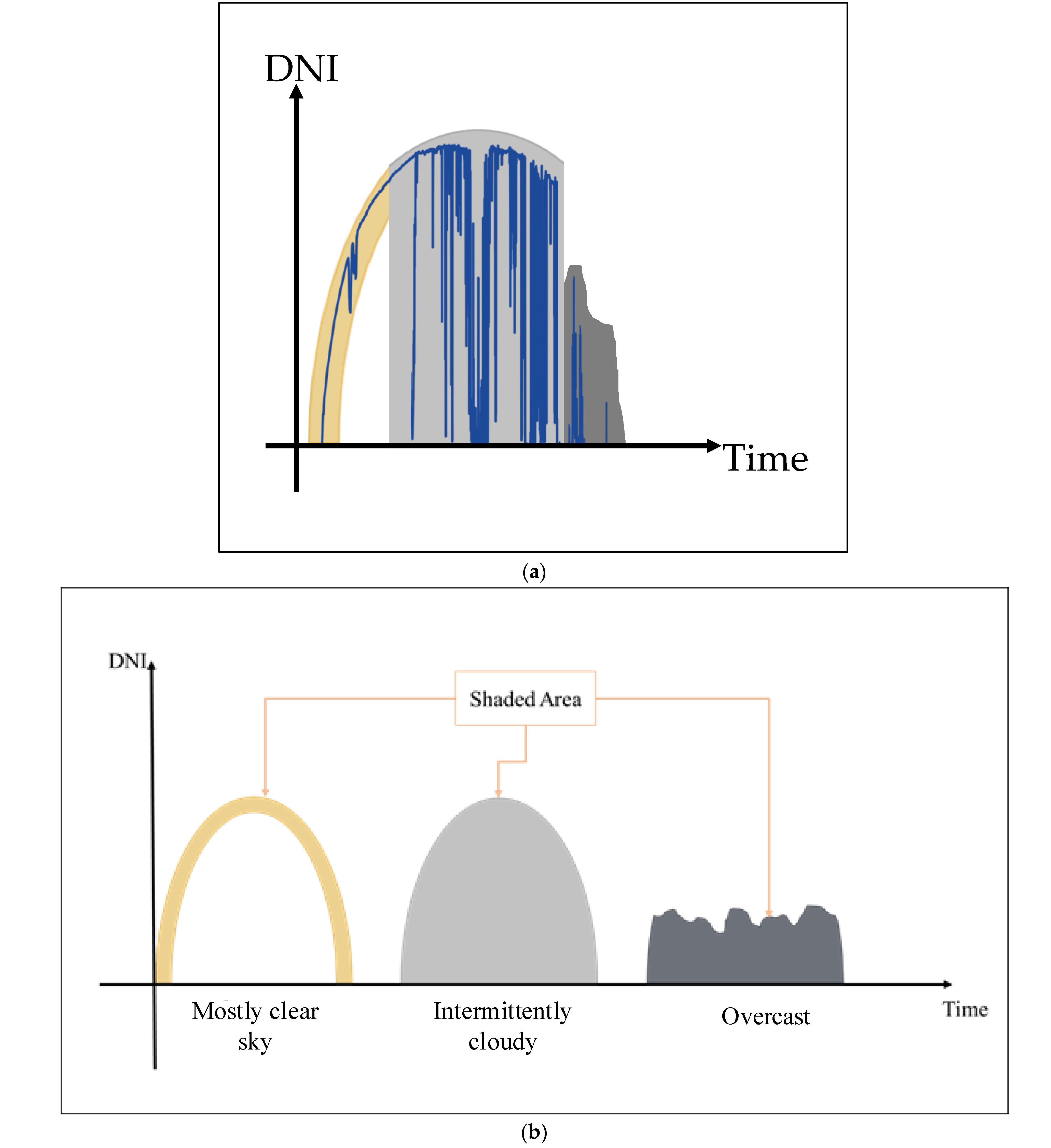
A further performance evaluation of the ASI system at Murdoch University under different conditions was conducted. These conditions were classified into three categories; mostly clear sky, intermittently cloudy, and overcast. The DNI MADs and DNI RMSDs of each class were then compared to the other five sites.

Comparing the descriptions of the three classes presented in Table 4 to the descriptions of the eight DNI variability classes by Nouri et al. [25], in

Table 8. Descriptions of the eight DNI variability classes by Nouri et al. [25].

Class	Description of Temporal DNI Variability
1	Clear sky conditions with low temporal DNI variability and very high clear sky index
2	Almost clear sky with low temporal DNI variability and high clear sky index
3	Almost clear sky with intermediate temporal DNI variability and high/intermediate clear sky index
4	Partly cloudy with high temporal DNI variability and intermediate clear sky index
5	Partly cloudy with intermediate temporal DNI variability and intermediate clear sky index
6	Partly cloudy with high temporal DNI variability and low/intermediate clear sky index
7	Almost overcast with intermediate temporal DNI variability and low clear sky index
8	Overcast with low temporal DNI variability and very low clear sky index

, the three classes in Table 4 were matched as shown in

Table 9. Matched classes for comparison.

Class from Table 4	Matched Classes from Table 8
1 (mostly clear sky)	1–3
2 (Intermittently cloudy)	4–6
3 (Overcast)	7–8

. However, it should be noted that there are differences in the variability classification methodologies employed for the Murdoch University site and employed for the other five sites. For Murdoch University, the classification was conducted by determining the classes using hourly sliding windows over a day and recording the most occurring class as the overall class of the day as explained in Section 3 of this study, whilst the classification of the other five sites involved the classification of every timestamp, using 15 min windows over a day and then categorising them as shown in Table 8 [25]. The matches in Table 9 were formulated by summarising the eight classes in Table 8 into: mostly clear sky (the sky is clear/almost clear, and the clear sky index is high), intermittently cloudy (the sky is partly cloudy, and the clear sky index is intermediate), and overcast (the sky is overcast/almost overcast, and the clear sky index is low). From the class descriptions, there is a possibility that classes 3 and 6 from Table 8, could be fitted into classes 2 and 3 from Table 4, respectively; however, in this study, these were matched as presented in Table 9.

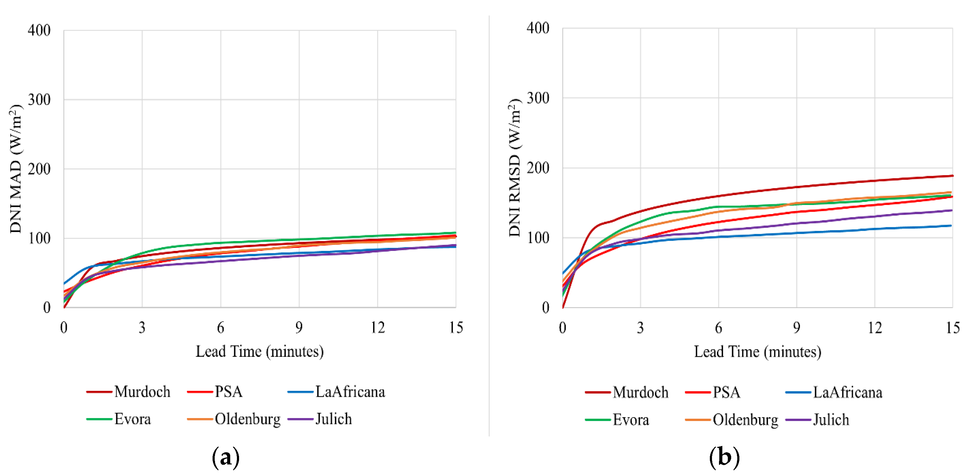
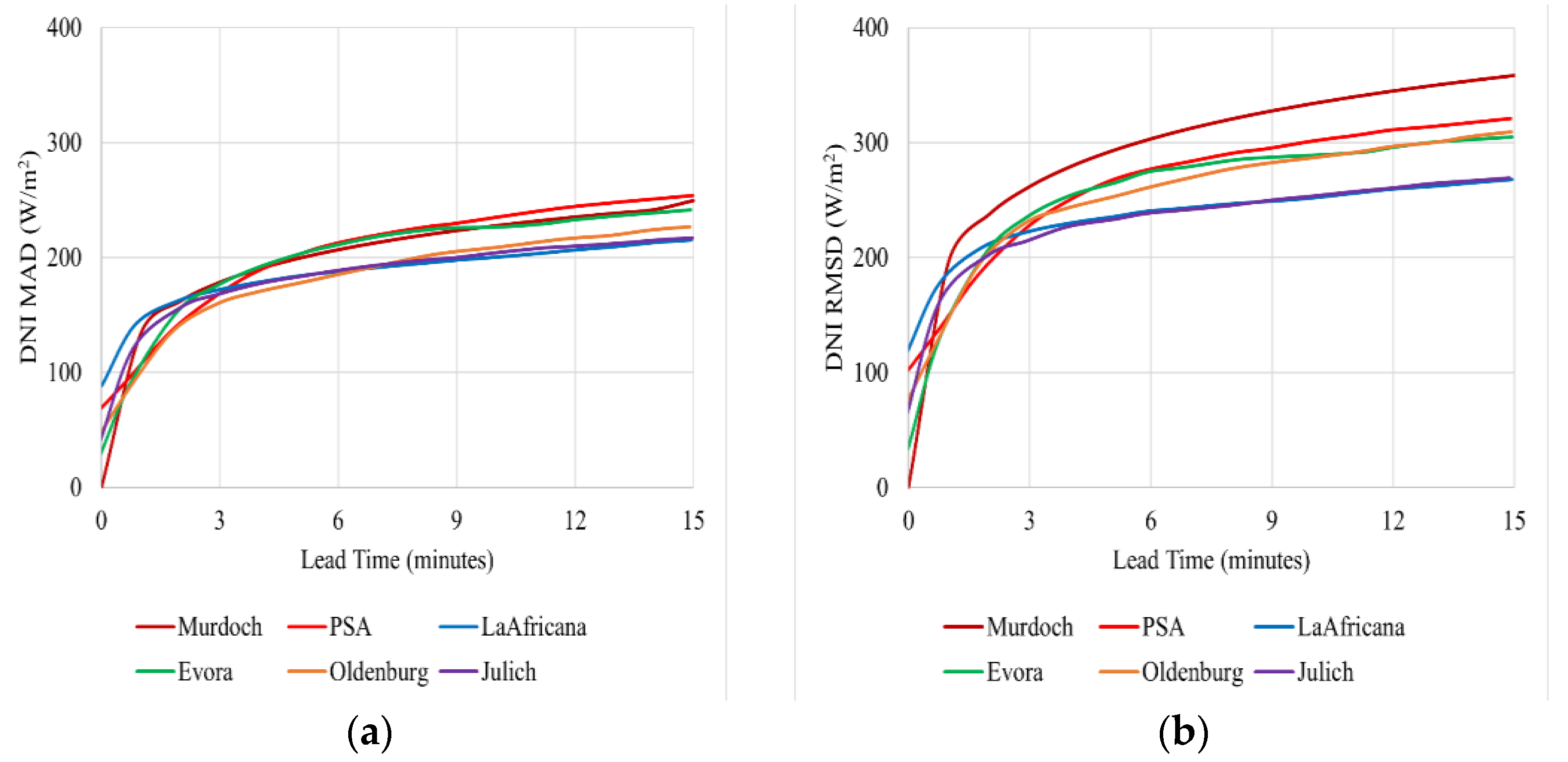
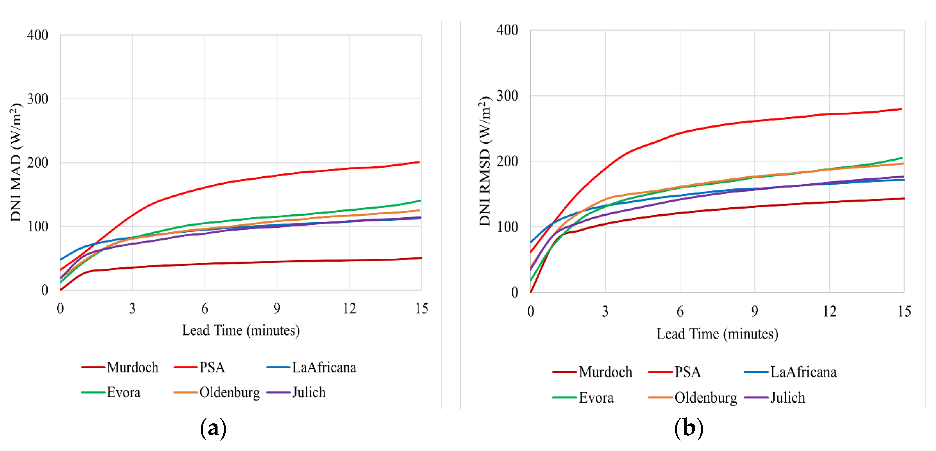
The DNI MADs and DNI RMSDs for classes 1 and 2 for Murdoch are showing an alignment with the results from PSA, La Africana, Evora, Oldenburg, and Julich, as shown in Figure 15, Figure 16 and Figure 17. From Figure 17a,b, it is seen that in overcast conditions (Class 3), the nowcasting system at the Murdoch University site displays the least DNI MAD and DNI RMSD of 50 W/m² and 148 W/m², respectively, whilst the DNI MAD and DNI RMSD for PSA for overcast conditions are relatively higher compared to the other six sites. The reason for this is that PSA is in a valley surrounded by mountains. When it is overcast, PSA records a lot of thin high layer cirrus clouds with complex multilayer conditions, resulting in higher uncertainties in cloud segmentation and tracking. Contrarily, when overcast, Perth observes low-layer stratus clouds, which are easy to process, resulting in a higher forecasting accuracy under such conditions.

The variations in DNI MADs and DNI RMSDs are also dependent on the sites’ proximity to the ocean, resulting in coastal cloud formations. The closer a system is to the coast, the higher the frequency of clouds, leading to increased intermittently cloudy conditions [39,40,41]. To investigate the effect of the location of an ASI nowcasting system with respect to the coast, an analysis of LT15 RMSDs for the intermittently cloudy class was conducted, and the results are displayed in

Table 10. ASI system’s distance from the nearest coast and LT15 RMSD.

ASI System Site	Approximate Distance from Nearest Coast (km)	LT15 RMSD (W/m2)
Murdoch	8.56	359
PSA	28.97	321
Oldenburg	62.29	310
Evora	81.87	305
La Africana	132.46	268
Julich	199.13	269

. It is observed from Table 10 that the LT15 RMSD decreases as the site distance from the coast increases, and these results are also complimented by Figure 16b.

5. Conclusions and Future Works

The integration of nowcasting systems in the control of IMGs might enable increased PV penetration levels, reduced spinning reserve requirements, and reduced fossil fuel usage. Such a system is installed at Murdoch University. In this study, nowcasts of 47 days’ worth of data were utilised to evaluate the performance of an ASI nowcasting system at Murdoch University in Perth, Western Australia (WA). DNI and GHI maps with edge lengths of 8 km and lead times up to 15 min ahead were generated.

The RMSD and MAD values were calculated as functions of variability classes and lead times. A simplified classification model, comprising three classes was developed and used for the classification exercise. Both the MAD and RMSD are relatively low for classes 1 (Mostly clear sky) and 3 (Overcast) as opposed to class 2 (Intermittently cloudy days). These results are consistent as these two classes (1 and 3) display low temporal irradiance variability, whilst class 2 displays high temporal irradiance variability. From the trends outlined in these results, it could be concluded that the simplified developed classification model works comparable with the one with eight classes. Additionally, for the integration of nowcasting into the control of IMGs, the distinction between mostly clear sky, overcast, and intermittently cloudy conditions, is sufficient, thus complementing the applicability of the simplified model. The overall performance of the nowcasting system was therefore as expected as it is consistent with previous evaluations in five other different sites namely PSA, La Africana, Evora, Oldenburg, and Julich. As a limitation, it should be noted that for the ASI system at Murdoch University, the number of overcast days (class 3) is very low, 6, compared to 17 and 24 for classes 1 and 2, respectively. Additionally, a performance comparison of different sites is difficult, even when the same classification methodology is applied due to the availability of different datasets.

However, the discretization of the dataset into three temporal irradiance variability classes does not take into account all effects that influence the nowcast performance such as the cloud heights and zenith angles, which can be considered as future work. Additionally, future work can be conducted on the possibility of integrating this nowcasting system with the control of IMGs in which solar PV is a part of the generation mix and examine if there is a possibility of enabling a higher solar PV penetration due to this control strategy.