Article

Efficient Simulation of Sandbody Architecture Using Probability Simulation—A Case Study in Cretaceous Condensate Gas Reservoir in Yakela Area, Tahe Oilfield, China

1
School of Earth Resources, China University of Geosciences, Wuhan 430074, China
2
Sinopec Northwest Oilfield Company, Urumqi 830011, China
*
Author to whom correspondence should be addressed.
Energies 2022, 15(16), 5971; https://doi.org/10.3390/en15165971
Submission received: 16 July 2022 / Revised: 7 August 2022 / Accepted: 16 August 2022 / Published: 18 August 2022
(This article belongs to the Section H1: Petroleum Engineering)

Abstract

:
The Cretaceous condensate gas reservoir in Yakela is in a fan delta system in which the river channel swings frequently and the contact relationships between sandbodies are complicated both vertically and horizontally. Therefore, making the sandbody architecture clear is becoming the most urgent demand in locating the remaining oil. However, conventional well correlations and fine interpretation do not apply in this area due to the large-spacing of wells and the lack of reliable seismic data. In this paper, we analyzed the vertical characteristics of sandbody architecture including the type and thickness of architectural elements and their contact relationships based on well data, then simulated the lateral and planar distribution probabilities via a database containing a large number of dimension parameters from relevant architectural elements using Monte Carlo simulation. This simulation provides reasonable and efficient estimation of inter-well sandbody distribution. The workflow and data we present can be applied to similar clastic reservoir modeling and simulations, especially for areas with insufficient well and seismic data.

1. Introduction

Sandbody architecture (also known as reservoir architecture, sandbody geometry, or reservoir heterogeneity) analysis is one essential method for clastic reservoir modeling, especially in the late stage of oil/gas field development, to locate the remaining oil/gas [1,2,3,4,5,6,7,8,9]. Sandbody architecture research originated from outcrop anatomies and aimed to provide data on the background sedimentary facies, environments, and evolutions of a specific reservoir [10,11,12]. With the development of subsurface techniques such as well logging, seismic, radar, and lidar, integrated with outcrop achievements, researchers have been marching towards realistic reconstructions of genetic stratigraphy and reservoir architecture in costal/shelf and fluvial reservoirs, specifically in meandering river systems [13,14,15,16,17,18,19,20,21,22]. Meanwhile, in fan delta reservoirs, the sediment commonly consists of a high proportion of coarse material that is seasonally transported through a series of distributary channels of braided river, and thus is more complicated in sandbody distribution and connection compared to marine reservoirs or fluvial systems [10]. As a result, deltaic reservoirs had not been examined in the aspect of architecture as thoroughly as shelf reservoirs or meandering river channels until recent years [23,24,25].
From previous research we can conclude the prerequisites of reservoir architecture analysis are finely described outcrops, closely spaced wells, or seismic data with high resolution and accuracy. Thus, it is challenging to carry out the fine characterization of reservoir architecture in areas of widely spaced wells with no reliable seismic data.
The Yakela Cretaceous condensate gas reservoir (YKL), which has been producing stably for over 20 years, is the largest self-contained condensate gas reservoir of Sinopec and one of the sources of gas transportation from the west to the east in China [26]. With the deepening of fine development, it is urgent to make the distribution characteristics of the reservoir clear. Unfortunately, in this area the well spacing is large (the average distance is ~1500 m compared to 150~300 m in a fluvial reservoir), and the seismic data is of poor quality due to the harsh operating environment (high latitude Gobi Desert) and complicated subsurface structure (multiple severe tectonic movements in buried history). Under these conditions, it is exceedingly difficult to estimate the reservoir architecture and obtain a reliable reservoir model.
Here we present a feasible and reasonable workflow for reservoir architecture estimation under the circumstance of lacking well and seismic data. According to Walther’s Law of facies, which states that the vertical succession of continuous sedimentary facies reflects lateral changes in their environment [27,28], it is possible to estimate the lateral developments from the limited data of vertical characteristics through reasonable simulation. We first summarize the vertical distribution probabilities of the target reservoir based on cores, well logs, and test data, and then carry out a Monte Carlo simulation using the vertical distribution probability through a training model of reservoir architectural elements to estimate the spatial distribution probability of the reservoir elements in the study area. The simulation’s result is validated by the later seismic-interpretated reservoir model. This efficient simulation can be further applied to similar fan delta reservoirs to improve or validate the accuracy of reservoir modeling.

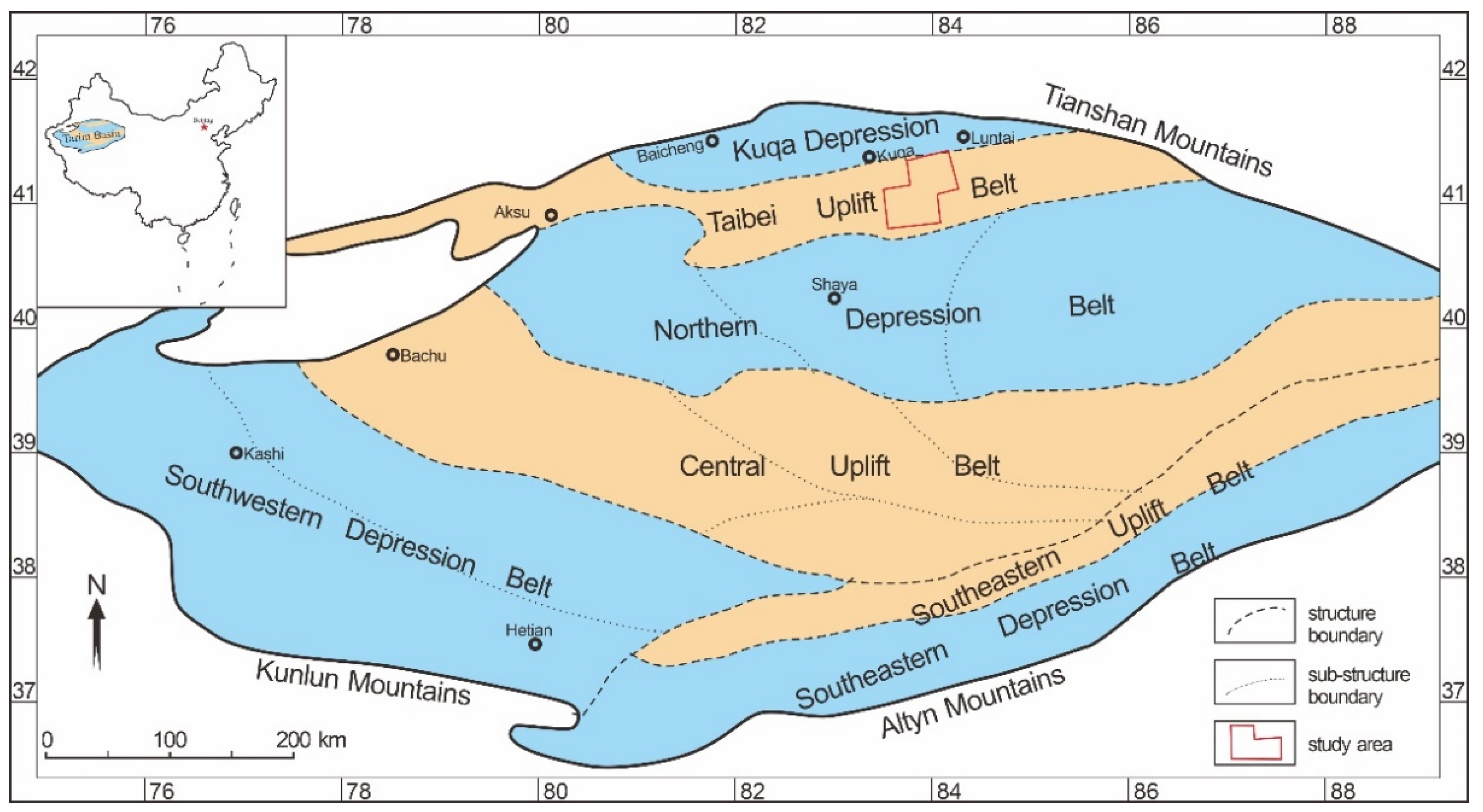
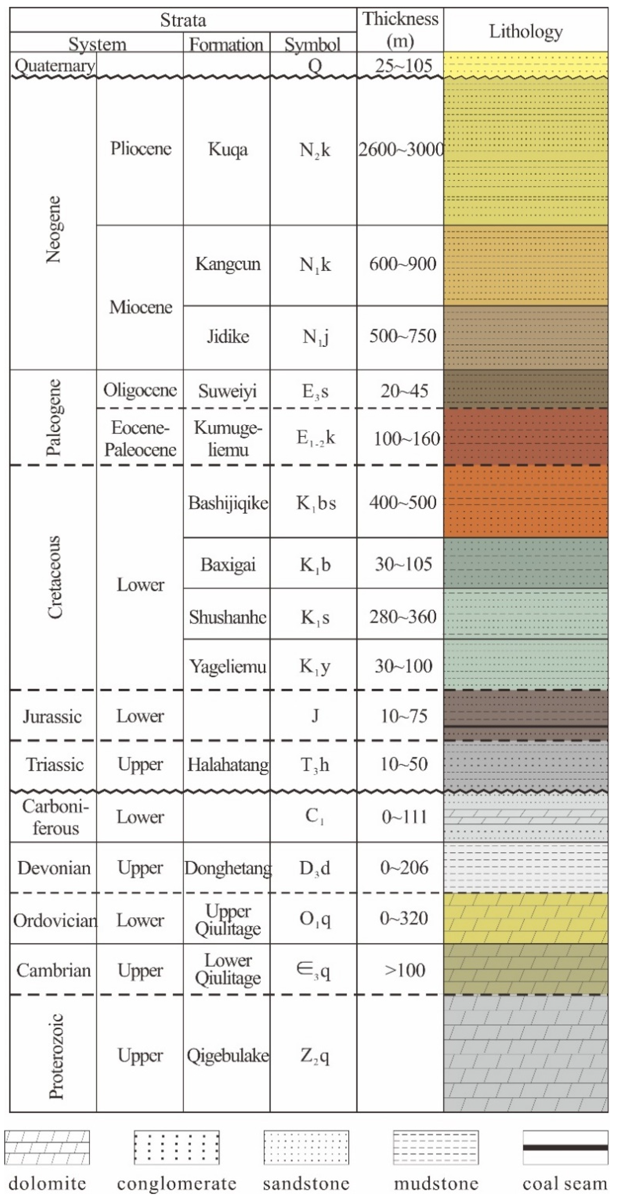
2. Geological Background

The Tarim Basin in northwestern China covering an area of 560,000 km2 and is the largest petroliferous basin in China. This basin can be divided into seven structural zones, including the Kuqa depression, the Taibei Uplift Belt, the Northern Depression Belt, the Central Uplift Belt, the Southwestern Depression Belt, the Southeastern Uplift Belt, and the Southeastern Depression Belt [29,30,31,32]. The Yakela gas reservoir is in the Yakela sag in the Taibei Uplift Belt (Figure 1).
The strata revealed in the study area include (from bottom to top) Proterozoic, Upper Cambrian, Lower Ordovician, Upper Devonian, Lower Carboniferous, Upper Triassic, Lower Jurassic, Lower Cretaceous, Paleogene, Neogene, and Quaternary (Figure 2). The target layer of this research is the clastic reservoir in the Cretaceous Yageliemu Formation (K1y).
The K1y condensate gas reservoir has a gas-bearing area of 38.6 km2. It is a normal temperature and pressure system with deep burial depth (>5300 m), no oil ring, medium condensate content (~234 g/m3), a large water body (~100 times), low porosity (10–15%), and medium-to-low permeability (10–150 mD). There are, in total, 43 wells in this area, with a minimum well spacing of 234 m and an average well spacing of ~1500 m. This well spacing is quite large compared to the average value of 100~200 m in previous sandbody architecture research. Regional sedimentary facies studies suggest that the K1y reservoir can be divided into the lower transgressive lake fan delta and the upper regressive braided river delta sedimentary systems, and that the microfacies include braided distributary channels, distributary channels, flood plains, inter-distributary bay, and sand bars [6,33].

3. Methodology

The overall methodology is first summarizing the vertical distribution probability of reservoir architectural elements as a testing dataset, then building a reservoir architectural element database as a training dataset for a Monte Carlo simulation, and finally, applying the testing dataset in the simulation model to get the horizontal distribution probability of the reservoir (Figure 3).

3.1. Reservoir Data Preparation

Well data of study area include core measurements of porosity and permeability (138 data sets), core observations (23 wells, 253 m in total), and well logs (SP, GR, AC, DEN, R, CNL for 39 wells). We used these data to analyze the microfacies and determine the parameters of architectural elements, including thickness, vertical contact relationships, and horizontal distances between wells. The vertical architectural element parameters then served as the testing dataset for the probability estimation of sandbody development and distribution.

3.2. Building Sandbody Architectural Element Database

As the well data primarily reveal vertical distribution characteristics, we introduced multiple analogue data to build a sandstone architecture database containing the length, width, and thickness of sandbodies. This database served as training dataset on sandbody development and distribution probability. The analogue data include measured dimensions of modern sand bars, similar reservoirs, and outcrop sections.

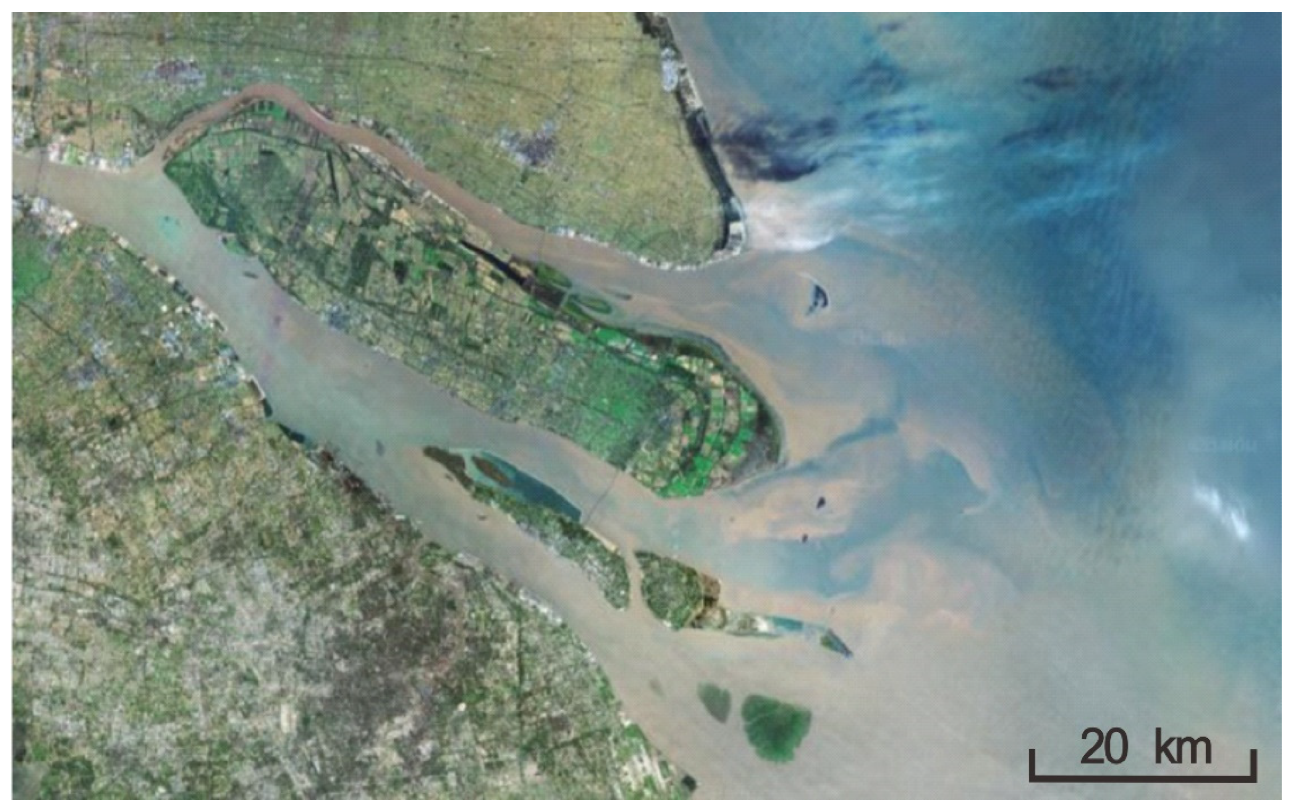
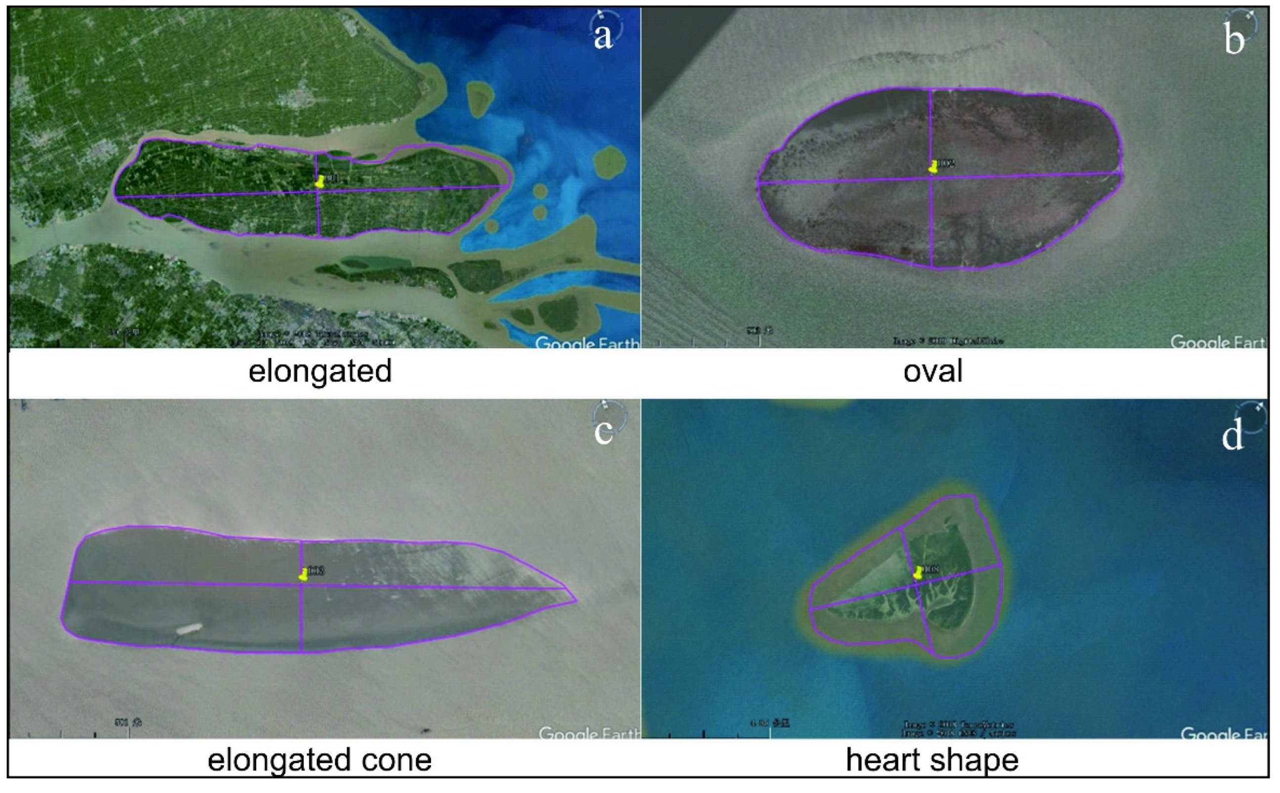
3.2.1. Modern Sand Bars

We observed and measured the satellite images of the Yangtze River Delta in the Google Earth satellite map (Figure 4), then analyzed the planar geometric and morphological characteristics of the sandbars at the Yangtze River mouth. The channel at the estuary of the Yangtze River Delta has a large amount of sediment of significant width, indicating a fast sediment-deposition rate. The estuary sandbars are formed primarily by sedimentation and river erosion, with few disturbances by human activities. According to the results of measurement and statistics, the sandbars can be categorized into four shapes (Figure 5): (1) Elongated, the sandbar is strip-shaped (the ratio of length to width greater than 3), and the rear of the sandbar is flat; (2) Oval, the two ends of the sandbar are approximately arc-shaped, and the whole body looks like an oval shape; (3) Elongated cone, one end of the sand dam is flat, and the other one is of a triangle shape. The length to width ratio of the sand dam is greater than 3; (4) Special shapes, some of the sandbars are more complex in shape and can be categorized to special shapes. The measurement results of the shape, area, length, and width of each sandbar show that oval is the common shape of the sandbars, the length of the sandbars ranges in 400–600 m, and the width is mainly distributed 50–300 m (Table 1).

3.2.2. Similar Reservoir—Triassic Fluvial Reservoir of Block 1 in Tahe Oilfield

The stratigraphic structure and lithological properties of the K1y reservoir are similar to the braided river delta deposition of the Lower Triassic reservoir of Block 1 in Tahe Oilfield. The Lower Triassic reservoir in Block 1 uses fine seismic interpretation and well logs to discriminate the sandbody boundary. The sandbars in Block 1 are mainly spindle-shaped, with lengths ranging from 200–500 m and widths ranging from 200–400 m (Table 2).

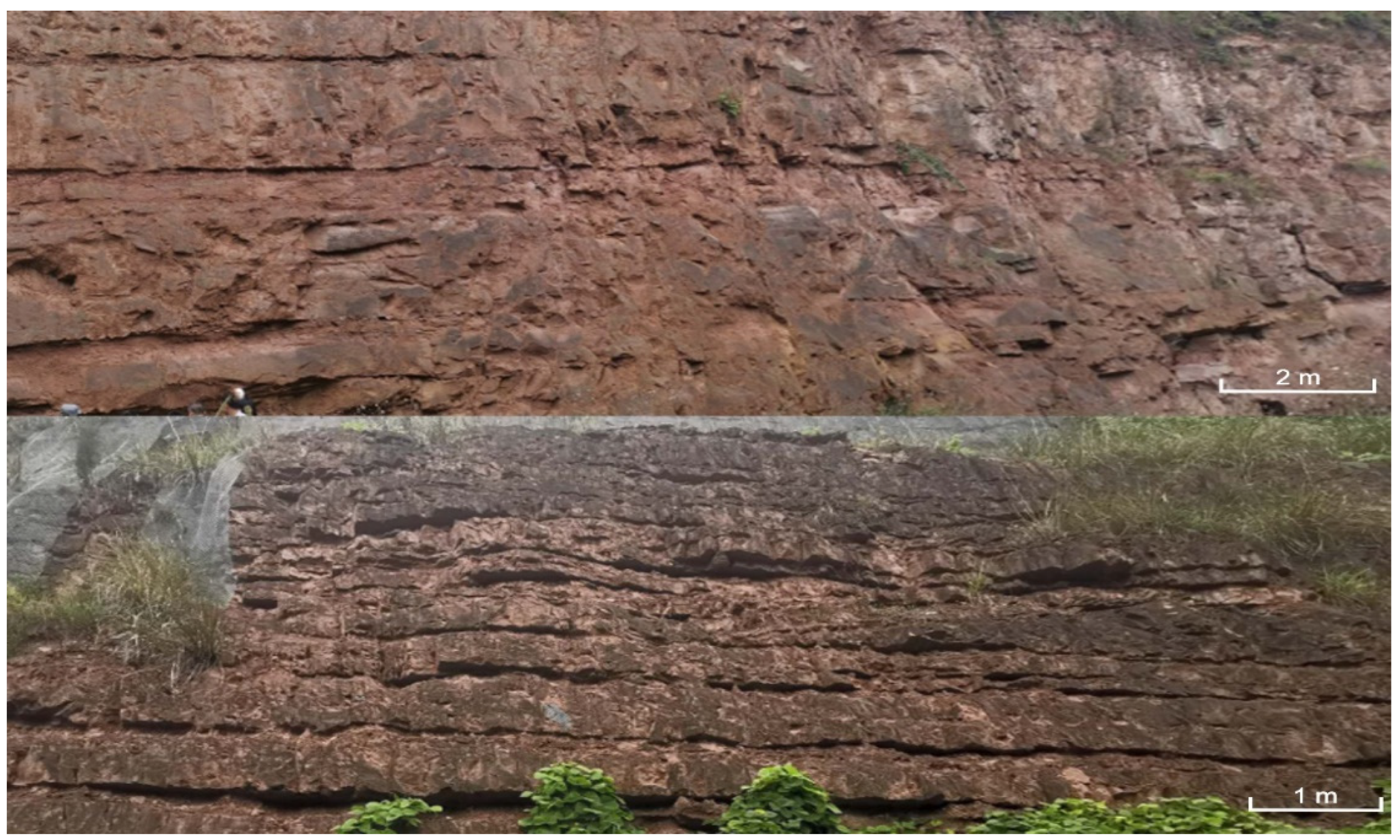
3.2.3. Outcrop Sections

We employ a set of sandstone architecture parameters based on field measurements of the Jurassic delta front outcrops in Yichang (central China), which had a complete exposure due to construction digging and thus can be tracked horizontally and vertically (Figure 6). The thickness of the sandbar of the delta front ranges from 1.5–2.1 m with an average value of 1.7 m, the width 11–22 m averaged at 17 m, and the width-to-thickness ratio is 7.5–12, averaged at 9.6 (Table 3). In addition, we summarized outcrop measurements from previous published articles to have more references for the lateral development characteristics of sandbodies.

3.3. Monte-Carlo Simulation

In this study, we used the Monte Carlo method to simulate the probability distributions of the reservoir dimensions and the contacting relationships based on Walther’s Law, i.e., the lateral extension and connection of sandbodies can be estimated through the vertical development characteristics. Monte Carlo simulations are used to model the probability of different outcomes in a process that cannot easily be predicted due to the intervention of random variables. It is also referred to as a multiple probability simulation. The essential idea of the Monte Carlo method is using randomness to solve problems that might be deterministic in principle [34]. The basis of a Monte Carlo simulation is that the probability of varying outcomes cannot be determined because of random variable interference. Therefore, a Monte Carlo simulation focuses on constantly repeating random samples to achieve certain results.
A Monte Carlo simulation takes the variable that has uncertainty and assigns it a random value. The model then runs, and a result is provided. This process is repeated again and again while assigning the variable in question many different values. Once the simulation is complete, the results are averaged together to provide an estimate. This method has been used in reservoir engineering calculations such as oil reserve estimation [35,36,37], and we believe more applications of the Monte Carlo simulation can be made as big data technology develops. The Monte Carlo simulation program we use is the embedded program in MATLAB. The data settings can be seen in Table 4. We carried out testing runs using the thickness data of Block 1 to simulate the length and width, and the result matched 86.25% of the original ones, suggesting this simulation has a good fit and can be employed to estimate the spatial extensions of YKL sandbodies.

4. Results

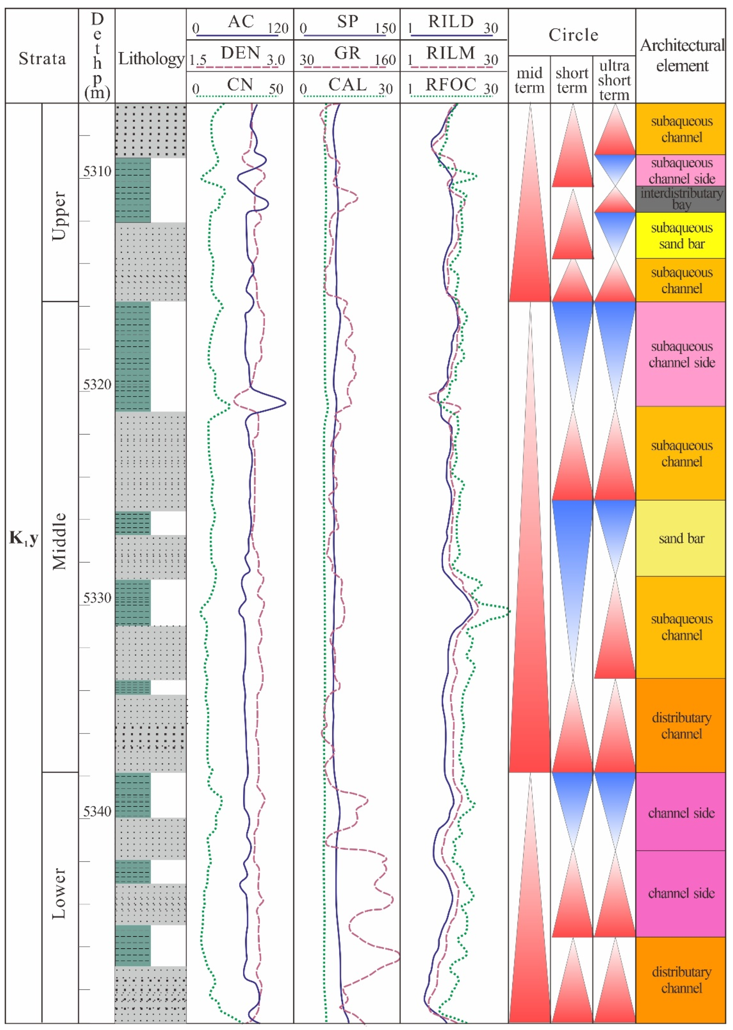
4.1. Architectural Elements Identification in Wells

As in previous research, the architectural elements developed in K1y of the study area include distributary channel, channel side, sandbar, interdistributary bay in delta plain, and subaqueous distributary channel, subaqueous channel side, subaqueous sandbar, and subaqueous interdistributary bay in subaqueous delta front, among which the subaqueous distributary channel is the most common element. Our work in this study was to establish the well logs interpretation from the lithofacies observed from cores (Table 5) and apply them to identify these architectural elements in each well. An example of architectural element determination can be seen in Figure 7.

4.2. Vertical Distributional Characteristics of Architectural Elements

We summarized the thickness portions of each architectural element and their vertical contact relationships in all the wells. These vertical distributional characteristics then served as a testing dataset for sandbody horizontal development estimation.

4.2.1. Thickness Portions of Architectural Elements

The probability distribution of the thickness portions of each architectural element in all the wells is shown in Figure 8. For the architectural elements of the fan-shaped delta plain, the distributary channel, channel side, sandbar, and interdistributary bay account for 38%, 21%, 12%, and 29%, respectively, making their ratios Distributary channel: sandbar: channel side: interdistributary bay ≈ 4:2:1:3. Among the architectural elements of the front edge of the underwater fan-shaped delta, the distributary channel accounts for 42%; and the sandbar, channel side, and interdistributary bay take up 29%, 13%, and 16%, respectively. The ratio of subaqueous distributary channel: sandbar: channel side: interdistributary bay ≈ 4:3:1:2.

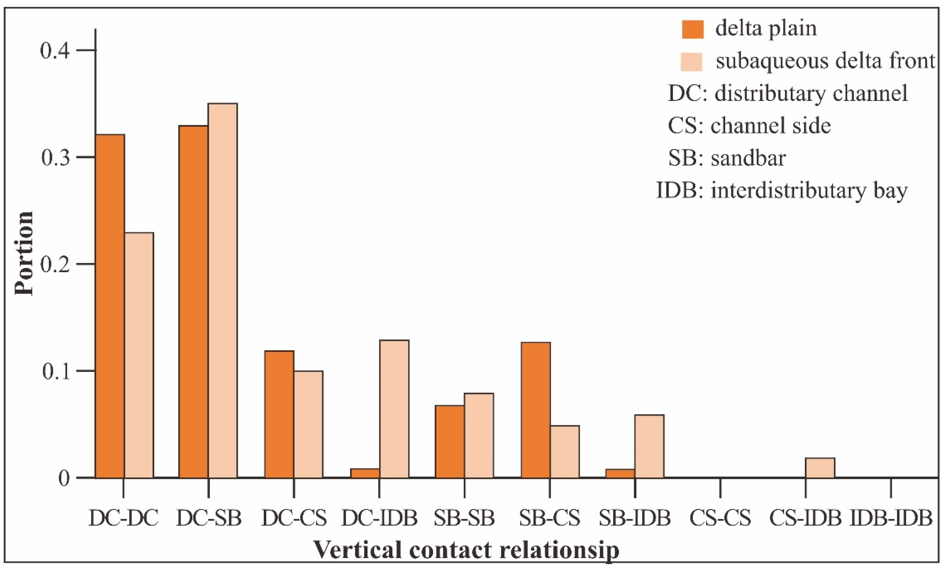
4.2.2. Vertical Contact Relationships and Their Portions

Three vertical contact (stacking) relationships of architectural elements were recognized in K1y reservoir: continuous stacking, intermittent stacking, and erosional stacking. Continuous stacking is the smooth vertical stacking through which sandbodies form a compete rhythm without mudstone interlayers. Intermittent stacking is similar to continuous stacking but with mudstone interlayers. Channel sedimentation maintenance complete sequence, with sandstones separated by sandbodies, and erosion superposition. Erosional stacking, also known as down-cut superposition, is the downward intrusion of a late-stage channel into an early-stage channel, resulting in superimposition of different sandbodies. The erosional stacking in appearance is similar to a single sandbody, whereas it often has multi-rhythmic combinations.
Calculated from the probability statistics of vertical contact relationships (Table 6), the ratio of continuous stacking: erosional stacking: intermittent stacking ≈ 4.5:4.3:1.2, indicating the most common vertical contact relationship of architectural elements is continuous stacking, while the intermittent stacking is rare. Further we summarized and compared the probabilities of all possible vertical combinations of any two architectural elements (Figure 9). The results show that distributary channel–distributary channel and distributary channel–sandbar are the most-common vertical combinations in both the delta plain and the subaqueous delta front, which means above and beneath a distributary channel would probably be a distributary channel or a sandbar. This is also one important rule for lateral contact relationship estimation following Walther’s Law.

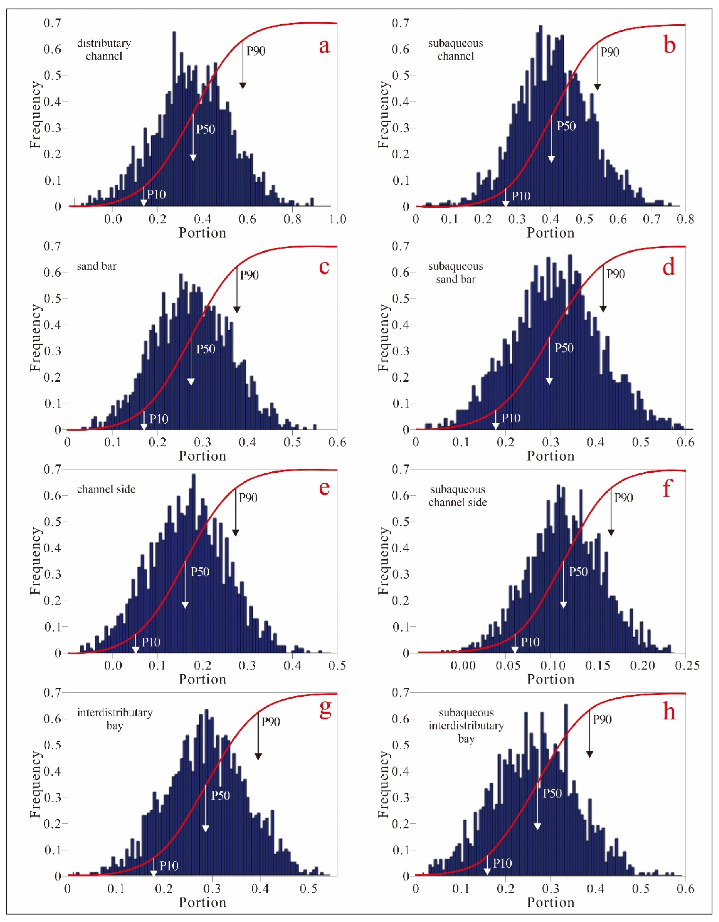
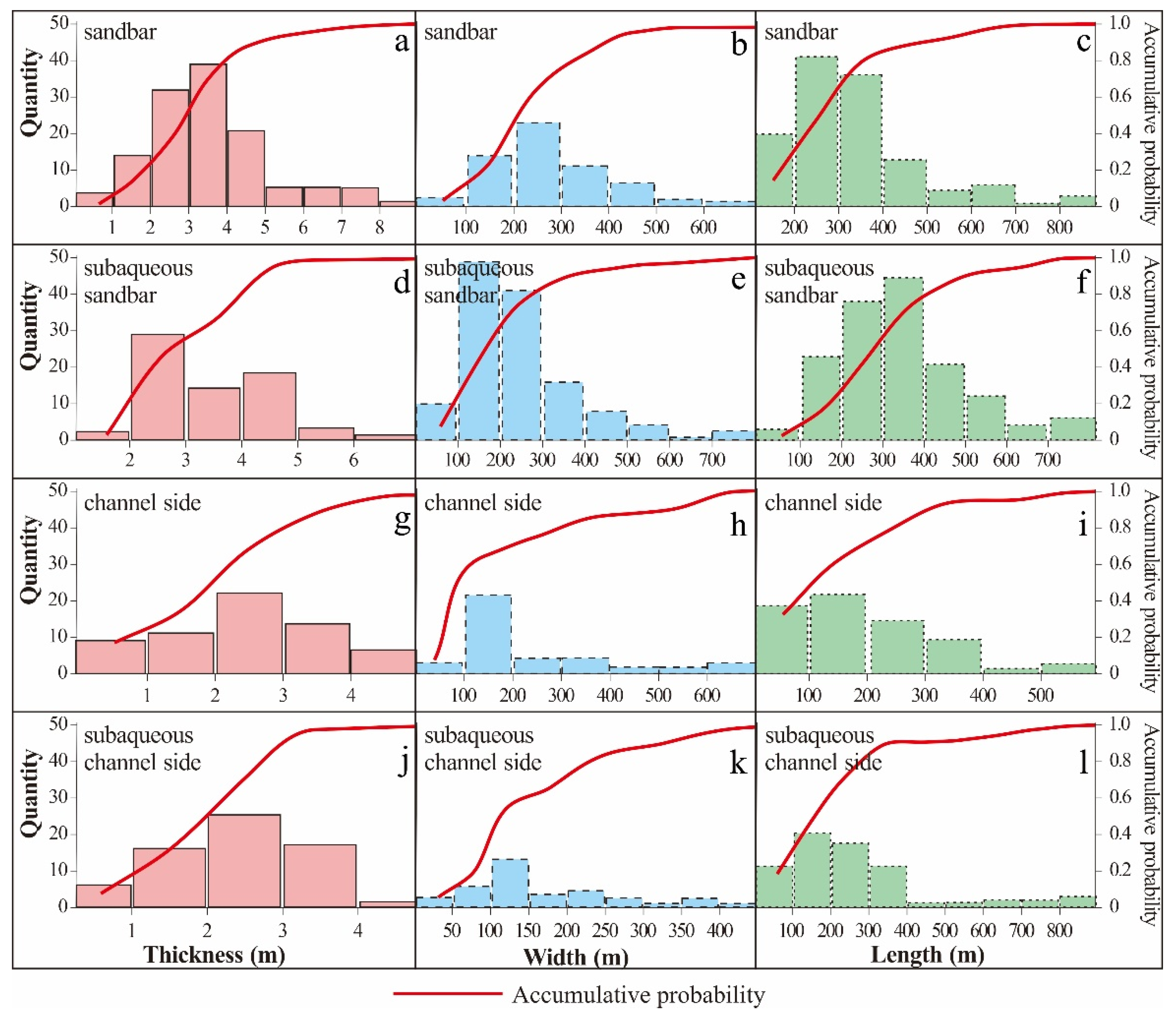
4.3. Probability Simulation of Sandbody Dimensions

The simulated probability of the horizontal (inter-well) extension of the sandbodies using the vertical distribution of the sandbar and channel side (two major reservoir types) is shown in Figure 10. The thickness of the sandbar is mainly distributed in the range of 1–5 m. The simulated width is mainly distributed in the range of 100–300 m and the simulated length ranges of 100–500 m (Table 7). For subaqueous sandbar, the thickness primarily ranges 2–5 m, and the simulated width and length probably ranges 100–300 m and 100–500 m, respectively. The simulated shape of the sandbars is mostly oval to elongate coned. The thicknesses of both the channel side and subaqueous channel side evenly distribute in the range of 1–4 m. The simulated width is limited to the range of 100–200 m, and the simulated length ranges 100–400 m. The shapes are elongated.

4.4. Simulated Reservoir Distribution Characteristics

4.4.1. Lateral Extension

Based on the simulated dimensions of sandbodies, we connected main production wells to form skeleton well sections. Viewed from the well sections, the subaqueous distributary channel of Lower K1y is thicker in two directions, and the range of the interdistributary bay is small. The subaqueous distributary channel and sandbar are the main elements; in Middle K1y the lake basin continued to expand, with strip-shaped and lens-shaped sandbar deposits developed. In Upper K1y water energy weakened but was relatively stable, so this horizon is dominated by fine-grained distributary channels, sandbars and channel sides. The distributary channel of the lower member of K1y is thicker in the south and north than in the center, and sandbars are wide in this member. The sandbars in the middle member are narrow and shaped lenticularly on sections, and the interdistributary bay and channel side develop on both sides of distributary channel, indicating the expansion of the lake basin. In the upper member, the grain size of the subaqueous distributary channel, sandbar, and channel side are smaller than that in the middle and lower member, indicating the weakening of water energy (Figure 11). The distributary channel and sandbar are the predominant architectural elements of sandbodies, making favorable reservoir property in this area.

4.4.2. Planar Distribution

The planar distribution characteristics vary in each layer of K1y, but the common rule is that the sandbodies have the axis of south–north (the regional depositional source direction), thus reservoir heterogeneity is strong in the west–east direction and in the eastern part the distributary channels is narrower comparing to those in the western part. Taking Layer 13 (the top layer of the lower member) for example, the subaqueous facies distribute in the southern part, where subaqueous sandbars are scattered and the subaqueous interdistributary bays are developed. In the northern part, the sandbars and channel sides are densely distributed, whereas interdistributary bay is rare (Figure 12). The area between S83 and YK9X dominantly developed subaqueous distributary channels, sandbars, channel sides, and interdistributary bays, indicating that the reservoir has good properties. Despite the producing wells, there are still good reservoirs yet to be explored.

5. Discussion

5.1. Validation of Sandstone Architecture Probability Simulation

New seismic data on the study area had been acquired one year after our work. Since the total thickness of K1y ranges 28~47 m, which is within or slightly thicker than a seismic wavelength, we still cannot get the fine description of reservoir distribution from the seismic interpretation. We tried to build the facies model through the comprehensive analysis of the amplitude, stacking velocity and other attributes, and adopted geobody interpretation, but it is not possible to specify the attributes to the meter-scale layers. We can check the area ranges of sandbodies and compare them with our simulated ones. We can see from the comparison of the model-extracted facies map and our simulated reservoir distribution map that our simulation results show a reasonable area coverage of sandbars comparing with the facies model (Figure 13).

5.2. Applicability of Reservoir Distribution Probability Simulation

As Miall commented in 2006 [6], a continuing effort to develop numerical simulation as the basis for reservoir engineering models is present. Common data on oilfields, such as cores and well logs, are the most direct data we can get for underground, but they are not enough for constraining reservoir models, especially the lateral extension of the reservoir. Hence, analogue and numerical simulation have long been the approaches for reservoir modeling. With the fast development of computer science and technics, we now are able to use big data and numerous simulation methods. What we need is more data, various detailed data of reservoir type, lithology, microfacies and their dimensions, etc. Our work is one effort towards big data and random simulation, and the result has been approved to some extent. We examine this approach to be the most appropriate method, at present, for reservoir distribution estimation in large well-spacing oilfields without proper seismic data.

5.3. Limitation of Probability Simulation

The limitations of our work include: (1) The study area is small, and the sedimentary circle is mid-term to ultrashort term, thus the application of this method to bigger environments needs further validation; (2) We have simulated the connection relationships between different architectural elements, whereas the specific or detailed connection patterns are not as delicate. It is our hope that we can visit more outcrops and obtain more high-resolution seismic profiles to enlarge our reservoir architecture database, then with the help of big data and random simulation, we can be more confident in reservoir architecture analysis and modeling.

6. Conclusions

Architectural elements and their contact relationships in a sandstone reservoir can be determined by core, well logs, and seismic profiles in the areas with sufficient well logging and high-resolution seismic data. However, for the widely spaced well areas without adequate seismic data, the study of reservoir architecture remains difficult. We have made progress in the area of Yakela using Monte Carlo simulation. The major conclusions include:
(1)
Well data in Yakela area provides the basic parameters of architectural elements and their contact relationships, based on which we obtained the statistical frequency of vertical developments of sandbodies and then used them as a testing dataset (variables) in the simulation of sandbody architecture.
(2)
We measured the sandbody dimensions of a modern sandbar, a similar reservoir, and outcrops and formed a comprehensive database. This database serves as a training dataset in the simulation of sandbody architecture.
(3)
We simulated the horizontal development probability of sandbodies in Yakela area from the testing dataset and built the reservoir model to locate favorable reservoir targets. This model fits well with the later seismic interpreted reservoir distribution, suggesting that our simulation is efficient and reliable.
(4)
It is of great significance to build a reservoir database with detailed dimensions and parameters of reservoir architectural elements (specific sandbodies). The larger the database is, the more powerfully those new technologies such as big data and deep learning can perform.

Author Contributions

Conceptualization, L.P. and X.W.; methodology, S.C. and T.D.; formal analysis, S.C. and X.W.; resources, H.L.; writing, S.C. and X.W.; project administration, L.P. All authors have read and agreed to the published version of the manuscript.

Funding

This research received no external funding.

Data Availability Statement

Not applicable.

Conflicts of Interest

The authors declare no conflict of interest.

References

  1. Pittman, E.D. Porosity, diagenesis and productive capability of sandstone reservoirs. In Aspects of Diagenesis; Schoue, P.A., Schluger, P.R., Eds.; SEPM Special Publication: Tulsa, OK, USA, 1979; Volume 26, pp. 159–173. [Google Scholar]
  2. Galloway, W.E. Reservoir facies architecture of microtidal barrier systems. AAPG Bull. 1986, 70, 787–808. [Google Scholar]
  3. Liu, K.; Boult, P.; Painter, S.; Paterson, L. Outcrop analog for sandy braided stream reservoirs: Permeability patterns in the Triassic Hawkesbury Sandstone, Sydney Basin, Australia. AAPG Bull. 1996, 80, 1850–1865. [Google Scholar]
  4. Karssenberg, D.; Tornqvist, T.E.; Bridge, J.S. Conditioning a process-based model of sedimentary architecture to well data. J. Sediment. Res. 2001, 71, 868–879. [Google Scholar] [CrossRef]
  5. Miall, A.D. Architecture and sequence stratigraphy of Pleistocene fluvial systems in the Malay Basin, based on seismic time-slice analysis. AAPG Bull. 2002, 86, 1201–1216. [Google Scholar]
  6. Miall, A.D. Reconstructing the architecture and sequence stratigraphy of the preserved fluvial record as a tool for reservoir development: A reality check. AAPG Bull. 2006, 90, 989–1002. [Google Scholar] [CrossRef]
  7. Hampson, G.J.; Sixsmith, P.J.; Johnson, H.D. A sedimentological approach to refining reservoir architecture in a mature hydrocarbon province: The Brent Province, UK North Sea. Mar. Pet. Geol. 2004, 21, 457–484. [Google Scholar] [CrossRef]
  8. Johannessen, P.N.; Nielsen, L.H. Architecture of an upper Jurassic barrier island sandstone reservoir, Danish Central Graben: Implications of a holocene-recent analogue from the Wadden Sea. Pet. Geol. Conf. 2010, 7, 145–155. [Google Scholar] [CrossRef]
  9. Siddiqui, N.A.; Ramkumar, M.; Rahman, A.H.A. High resolution facies architecture and digital outcrop modeling of the Sandakan formation sandstone reservoir, Borneo: Implications for reservoir characterization and flow simulation. Geosci. Front. 2019, 10, 957–971. [Google Scholar] [CrossRef]
  10. Galloway, W.E. Sediments and stratigraphic framework of the copper river fan-delta, Alaska. J. Sediment. Petrol. 1976, 46, 725–737. [Google Scholar]
  11. Miall, A.D. Reservoir heterogeneities in fluvial sandstones—Lessons from outcrop studies. AAPG Bull. 1988, 72, 682–697. [Google Scholar]
  12. Smith, R.D.A. Reservoir architecture of syn-rift lacustrine turbidite systems, early cretaceous, offshore south Gabon. In Geological Society Special Publication; Lambiase, J.J., Ed.; Geological Society Publishing House: Bath, UK, 1995; pp. 197–210. [Google Scholar]
  13. Richards, M.; Bowman, M. Submarine fans and related depositional systems ii: Variability in reservoir architecture and wireline log character. Mar. Pet. Geol. 1998, 15, 821–839. [Google Scholar] [CrossRef]
  14. Bruhn, C.H.L. Reservoir architecture of deep-lacustrine sandstones from the Early Cretaceous Recôncavo Rift Basin, Brazil. AAPG Bull. 1999, 83, 1502–1525. [Google Scholar]
  15. Clark, M.S.; Klonsky, L.F.; Tucker, K.E. Geologic study and multiple 3-D surveys give clues to complex reservoir architecture of giant Coalinga oil field, San Joaquin Valley, California. Lead Edge 2001, 20, 744–751. [Google Scholar] [CrossRef]
  16. Hornung, J.; Aigner, T. Reservoir architecture in a terminal alluvial plain: An outcrop analogue study (upper Triassic, southern Germany) part 1: Sedimentology and petrophysics. J. Pet. Geol. 2002, 25, 3–30. [Google Scholar] [CrossRef]
  17. Hampson, G.J.; Rodriguez, A.B.; Storms, J.E.A.; Johnson, H.D.; Meyer, C.T. Geomorphology and high-resolution stratigraphy of progradational wave-dominated shoreline deposits: Impact on reservoir-scale facies architecture. In Recent Advances in Models of Siliciclastic Shallow-Marine Stratigraphy; Hampson, G.J., Steel, R.J., Burgess, P.M., Dalrymple, R.W., Eds.; SEPM Special Publication: Tulsa, OK, USA, 2008; Volume 90, pp. 117–142. [Google Scholar]
  18. Sixsmith, P.J.; Hampson, G.J.; Gupta, S.; Johnson, H.D.; Fofana, J.F. Facies architecture of a net transgressive sandstone reservoir analog: The Cretaceous Hosta Tongue, New Mexico. AAPG Bull. 2008, 92, 513–547. [Google Scholar] [CrossRef]
  19. Sech, R.P.; Jackson, M.D.; Hampson, G.J. Three-dimensional modeling of a shoreface-shelf parasequence reservoir analog: Part 1. Surface-based modeling to capture high-resolution facies architecture. AAPG Bull. 2009, 93, 1155–1181. [Google Scholar] [CrossRef]
  20. Pyles, D.R.; Syvitski, J.P.M.; Slatt, R.M. Defining the concept of stratigraphic grade and applying it to stratal (reservoir) architecture and evolution of the slope-to-basin profile: An outcrop perspective. Mar. Pet. Geol. 2011, 28, 675–697. [Google Scholar] [CrossRef]
  21. Onyenanu, G.I.; Jacquemyn, C.E.M.M.; Graham, G.H. Geometry, distribution and fill of erosional scours in a heterolithic, distal lower shoreface sandstone reservoir analogue: Grassy Member, Blackhawk Formation, Book Cliffs, Utah, USA. Sedimentology 2018, 65, 1731–1760. [Google Scholar] [CrossRef]
  22. Mulhern, J.S.; Johnson, C.L.; Martin, J.M. Modern to Ancient Barrier Island Dimensional Comparisons: Implications for Analog Selection and Paleomorphodynamics. Front. Earth Sci. 2019, 7, 109. [Google Scholar] [CrossRef]
  23. Johnson, C.L.; Graham, S.A. Sedimentology and Reservoir Architecture of a Synrift Lacustrine Delta, Southeastern Mongolia. J. Sediment. Res. 2004, 74, 770–785. [Google Scholar] [CrossRef]
  24. Ambrose, W.A.; Hentz, T.F.; Bonnaffé, F. Sequence-stratigraphic controls on complex reservoir architecture of highstand fluvial-dominated deltaic and lowstand valley-fill deposits in the Upper Cretaceous (Cenomanian) Woodbine Group, East Texas field: Regional and local perspectives. AAPG Bull. 2009, 93, 231–269. [Google Scholar] [CrossRef]
  25. Deveugle, P.E.K.; Jackson, M.D.; Hampson, G.J. Characterization of stratigraphic architecture and its impact on fluid flow in a fluvial-dominated deltaic reservoir analog: Upper Cretaceous Ferron Sandstone Member, Utah. AAPG Bull. 2011, 95, 693–727. [Google Scholar] [CrossRef]
  26. Hu, W. Reservoir features and controlling factors of Yageliemu Formation in Yakela, Tarim Basin, China. J. Chengdu Univ. Technol. (Sci. Technol. Ed.) 2011, 38, 385–393, (In Chinese with English Abstract). [Google Scholar]
  27. Walther, J. Einleitung in die Geologie als historische Wissenschaft. In Lithogenesis der Gegenwart; G. Fischer, Bd.: Jena, Germany, 1894; Volume 3, pp. 535–1055. [Google Scholar]
  28. Middleton, G. Johannes Walther’s Law of Correlation of Facies. Geol. Soc. Am. Bull. 1973, 38, 979–988. [Google Scholar] [CrossRef]
  29. Zeng, L.; Wang, H.; Gong, L.; Liu, M. Impacts of the tectonic stress field on natural gas migration and accumulation: A case study of the Kuqa Depression in the Tarim Basin, China. Mar. Pet. Geol. 2010, 27, 1616–1627. [Google Scholar] [CrossRef]
  30. Lai, J.; Wang, G.; Chai, Y.; Xin, Y.; Wu, Q.; Zhang, X.; Sun, Y. Deep burial diagenesis and reservoir quality evolution of high-temperature, high-pressure sandstones: Examples from Lower Cretaceous Bashijiqike Formation in Keshen area, Kuqa depression, Tarim basin of China. AAPG Bull. 2017, 101, 829–862. [Google Scholar] [CrossRef]
  31. Yao, Z.; He, G.; Li, C.F.; Dong, C. Sill geometry and emplacement controlled by a major disconformity in the Tarim Basin, China. Earth Planet. Sci. Lett. 2018, 501, 37–45. [Google Scholar] [CrossRef]
  32. Wang, T.F.; Jin, Z.; Li, H.; Liu, D.; Cheng, R.; Shi, S.; Wang, J. Processes and causes of Phanerozoic tectonic evolution of the western Tarim Basin, northwest China. Pet. Sci. 2020, 17, 279–291. [Google Scholar] [CrossRef]
  33. Liang, L.; Gao, Y.; Zhang, H.; Shao, G.; Yin, T.; Ding, H. Sedimentary Microfacies Analyses of Yageliemu Formation of Yakela Condensate Gas Field in Southern Tianshan Area of Tarim Basin. Xinjiang Geol. 2013, 31, 66–71, (In Chinese with English Abstract). [Google Scholar]
  34. Kroese, D.P.; Taimre, T.; Botev, Z.I. Handbook of Monte Carlo Methods. In Wiley Series in Probability and Statistics; John Wiley & Sons: New York, NY, USA, 2011. [Google Scholar]
  35. Murtha, J.A. Monte Carlo simulation: Its status and future. J. Pet. Technol. 1997, 49, 361–373. [Google Scholar] [CrossRef]
  36. Cortazar, G.; Schwartz, E.S. Monte Carlo evaluation model of an undeveloped oil field. J. Energy Financ. Dev. 1998, 3, 73–84. [Google Scholar] [CrossRef]
  37. Ungerer, P.; Tavitian, B.; Boutin, A. Applications of Molecular Simulation in the Oil and Gas Industry: Monte Carlo Methods; Editions Technip: Houston, TX, USA, 2005. [Google Scholar]
Figure 1. Structural map of Tarim Basin and the location of the study area.
Energies 15 05971 g001
Figure 2. Stratigraphy column of study area.
Energies 15 05971 g002
Figure 3. Systematic workflow.
Energies 15 05971 g003
Figure 4. Location of modern sandbars for distant measurement.
Energies 15 05971 g004
Figure 5. Examples of the shape and measuremnt of morden sandbars.
Energies 15 05971 g005
Figure 6. Jurassic delta outcrop in Yichang.
Energies 15 05971 g006
Figure 7. Bounding surfaces’ discrimination and sandstone architectural element determination of a typical well in Yakela area.
Energies 15 05971 g007
Figure 8. Probability distributions of architectural elements in all wells showing best estimate (P50), high estimate (P10), and low estimate (P90). The delta plain elements are on the left and the corresponding subaqueous delta front elments are on the right. (a): distributary channel; (b): subaqueous channel; (c): sand bar; (d): subaqueous sand bar; (e): channel side; (f): subaqueous channel side; (g): interdistributary bay; (h): subaqueous interdistributar bay.
Energies 15 05971 g008
Figure 9. Vertical combinations of architectural elements and their portions.
Energies 15 05971 g009
Figure 10. Thickness and simulated lateral dimension of architectural elements. The red line shows the accumulative probability. (a): thickness probabity of sandbar; (b): width probability of subaqueous sandbar; (c): length probability of subaqueous sandbar; (d): thickness probabity of subaqueous sandbar; (e): width probability of subaqueous sandbar; (f): length probability of subaqueous sandbar; (g): thickness probabity of channel side; (h): width probability of channel side; (i): length probability of channel side; (j): thickness probabity of subaqueous channel side; (k): width probability of subaqueous channel side; (l): length probability of subaqueous channel side.
Energies 15 05971 g010
Figure 11. A typical well section showing the lateral extension of sandbodies. The location of this section is shown in Figure 11.
Energies 15 05971 g011
Figure 12. The facies map of a typical layer.
Energies 15 05971 g012
Figure 13. Comparison between the probability simulation results and the petrophysics determined facies model of the upper member of K1y in Yakela area.
Energies 15 05971 g013
Table 1. Detailed measurements of modern sandbars.
No.ShapeLength (m)Width (m)
01oval1364676
02elongated1879415
03Special shape: quadrilateral249198
04Special shape: fan shape785510
05oval19795
06oval836433
07Special shape: irregular500177
08Special shape: fan shape433246
09Special shape: quadrilateral430240
010oval1078370
011elongated cone873523
012Special shape: quadrilateral556533
013elongated cone489269
014elongated cone483198
015oval8024
016Special shape: leaf shape8621.4
017oval23155
018elongated15122
019elongated cone741276
020elongated cone438250
021elongated976309
022elongated cone453229
023elongated cone471224
024elongated cone492269
025elongated cone435168
Table 2. Interpreted dimensions of sandbars in Block 1.
No.ShapeLength (m)Width (m)Thickness (m)
1elongated cone6723218.1
2elongated cone5162637.44
3elongated cone3812304.86
4elongated cone4232095.56
5elongated cone5002727.15
6elongated cone4292316.8
7elongated cone4282078.86
8elongated cone4282095.92
9elongated cone5363307.92
10elongated cone7313618.7
11elongated cone6112698.38
12elongated cone78030710.42
13elongated cone5402548.32
14elongated cone492.75238.55.28
15elongated cone4253299.5
16elongated cone5652875.06
17elongated cone4652678.22
18elongated cone5172586.2
19elongated cone5033158.22
20elongated cone4822524.96
21elongated cone4272488.52
22elongated cone3292127.44
23elongated cone78040710.42
24elongated cone5403548.32
25elongated cone6593929.28
26elongated cone51539610.96
27elongated cone64145912.18
28elongated cone66229710.34
29elongated cone57838311.05
30elongated cone49934310.06
31elongated cone57335710.92
32elongated cone69442113.32
Table 3. Measurements of Jurassic delta from outcrop sections in Yichang.
Sandbody TypeShapeWidth (m)Thickness (m)
River mouth barconvex lenticular
(both top and bottom surfaces)
11.21.5
18.22.1
16.91.4
22.42.1
16.81.82
Subaqueous distributary channelconcave lenticular
(bottom surface)
7.61.4
22.42.8
16.12.1
70.9
81.2
192
234.5
distributary channelTop surface flat, bottom surface convex1101.5
823.7
1553
1155.8
894
883.3
Table 4. Settings of the Monte Carlo simulation.
ParametersSetting
InputThickness, contact code of YKL sandbodiesOriginal frequency distribution from well data
Length and width of modern sandbarStatistics from real data and forms the relationships of the three dimensions of sandbodies
Length, width, and thickness of analogue reservoir Block 1
Thickness and width of outcrops
OutputLength and width of YKL sandbodies
Number of runs1 × 106
Table 5. Lithofacies and well log interpretations of architectural elements.
Architectural ElementLithofaciesWell Log Facies
Fan delta plainDistributary channelFining upwardLow amplitude bell shaped/cylinder shaped Energies 15 05971 i001
SandbarCoarsening upwardFunnel shaped Energies 15 05971 i002
Channel sideInterlayering of sandstones and mudstonesHigh amplitude cylinder shaped Energies 15 05971 i003
Interdistributary bayMudstone predominant, containing conglomerate or thin sandstone layersMiddle-high amplitude folk shaped Energies 15 05971 i004
Fan delta frontSubaqueous distributary channelFining upward
(finer than distributary channel)
Low amplitude bell shape/cylinder shaped Energies 15 05971 i005
Subaqueous sandbarCoarsening upward
(finer than distributary channel)
Funnel shaped Energies 15 05971 i006
Subaqueous channel sideThin layers, interlayers of sandstones and mudstonesMiddle-high funnel shaped Energies 15 05971 i007
Subaqueous interdistributary bayMudstone predominant, occasional sandstone seamHigh amplitude fork shaped Energies 15 05971 i008
Table 6. Probability statistics of vertical contact relationships of architectural elements.
Vertical Contact RelationshipAccumulative Probability
P10P90P50
Continuous stacking0.330.580.45
Erosional stacking0.290.480.43
Intermittent stacking0.010.240.12
Table 7. Statistics of simulation results.
NameCountMeanErrorConvergence
SandbarLength468,5932523.55converged
Width586,4633912.56converged
Subaqueous sandbarLength732,5812061.51converged
Width696,5343522.64converged
Channel sideLength259,8671883.03converged
Width452,8982672.71converged
Subaqueous channel sideLength554,3961452.89converged
Width359,1222293.62converged
Publisher’s Note: MDPI stays neutral with regard to jurisdictional claims in published maps and institutional affiliations.

