Investigation of Liquid–Gas Flow in a Horizontal Pipeline Using Gamma-Ray Technique and Modified Cross-Correlation

Abstract

This article presents the application of the radioisotope absorption method in the study of two-phase water–air flow in a horizontal pipe. The measurement principle and the test stand are briefly described. The main part of the article presents the signal analysis methods applied to data obtained from scintillation detectors. Because these signals are mostly stochastic waveforms, they were analyzed statistically using the cross-correlation function (CCF), and methods that are a combination of CCF and differential methods: CCF/ASDF and CCF/AMDF, where ASDF is the average square difference function, and AMDF is the average magnitude difference function. Examples of the results of gas phase velocity measurement for four types of flow are presented. It was found that the CCF/ASDF and CCF/AMDF methods allow more accurate results of measurements of the dispersed phase to be obtained than the CCF method.

1. Introduction

In industries such as chemicals, energy, oil and methane mining, and environmental engineering, there is a need to transport two-phase liquid–gas mixtures. Control of this type of flow is often important in the course of industrial processes, and continuous technological development requires the improvement of the measurement techniques. Measurements of two-phase flow parameters in pipelines require the application of advanced, usually noninvasive techniques such as tomographic methods, particle image velocimetry, Coriolis flow meters, high-speed cameras, laser doppler anemometry, and magnetic resonance imaging [1,2,3,4,5,6,7]. For more than 50 years, research on this type of flow has utilised methods based on the introduction of radioactive isotopes into the flow under certain conditions (radiotracer method) or the application of closed gamma radiation sources (absorption method) [8,9,10,11,12,13,14]. It should also be mentioned that the formation and movement of air bubbles in a two-phase flow depends on many factors, that make the numerical calculations of such processes difficult [15]. This justifies the need for experimental control of such processes.

In this work, the gamma absorption method is used to designate the average velocity of air bubbles transported through water in a horizontal pipe. The research involved ²⁴¹Am gamma radiation sources and detectors with NaI(Tl) crystals. The study used the results of measurements obtained on an experimental set-up built to conduct tests on liquid–gas flows, simulating processes observed in the petrochemical industry. For the analysis of signals from scintillation detectors, the cross-correlation function (CCF) is used most often [16,17]. In this article, in addition to the classical CCF, the following differential methods were added: the average square difference function (ASDF) and the average magnitude difference function (AMDF). In this way, the combined CCF/ASDF and CCF/AMDF methods were developed.

Simulation studies of the combined methods were presented in the study [18]; while the study [19] described the application of these methods to the analysis of signals from the water–solid particle flow in a vertical pipeline.

In this work, combined methods were used to analyse signals from scintillation probes in the study of water–air flow in a horizontal pipe. This type of flow is different from the liquid–solid particle because a mixture of water–air creates characteristic structures in the flow [9].

This paper is a significantly extended version of conference publications [20,21].

2. Radioisotope Absorption Method

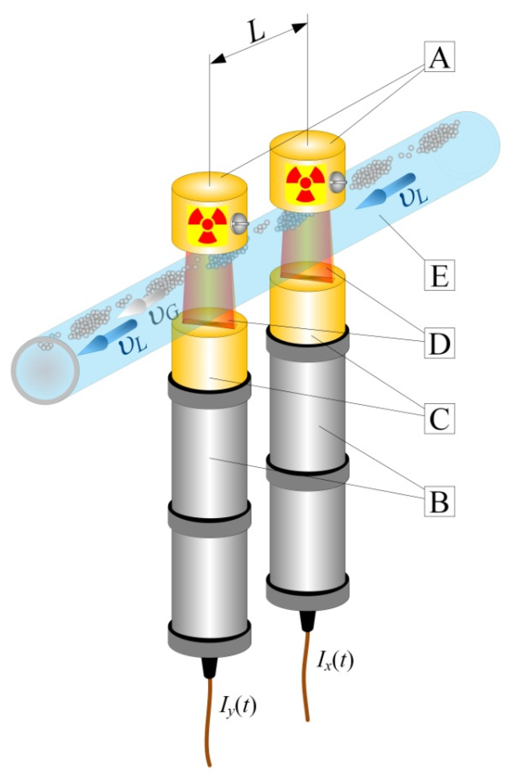
The principle of using gamma radiation absorption to measure the velocity of gas transport through a liquid in a horizontal pipeline is shown in Figure 1.

A typical absorption measurement set includes a closed gamma radiation source (A) and a scintillation detector (B) with appropriate collimators (A), (C). The combination of two sets deployed at a distance of L from each other allows the dispersed phase flow rate to be determined. The flow of the tested mixture through the pipeline (E) causes changes in absorption of gamma-ray beam (D) and allows mutually delayed stochastic signals to be obtained from the probes. Analysis of these signals by statistical methods, e.g., using cross-correlation [17], allows determination of transport delay τ₀ and the average velocity of air bubbles υ_G from the relation:

$${\upsilon }_G=\frac{L}{{\tau }_0}$$

(1)

where L = 97 mm is the distance of the probes.

If necessary, the liquid flow velocity υ_L can be determined using an ultrasonic flow meter, for example. In closed research installations, a radioisotope tracer method can also be used.

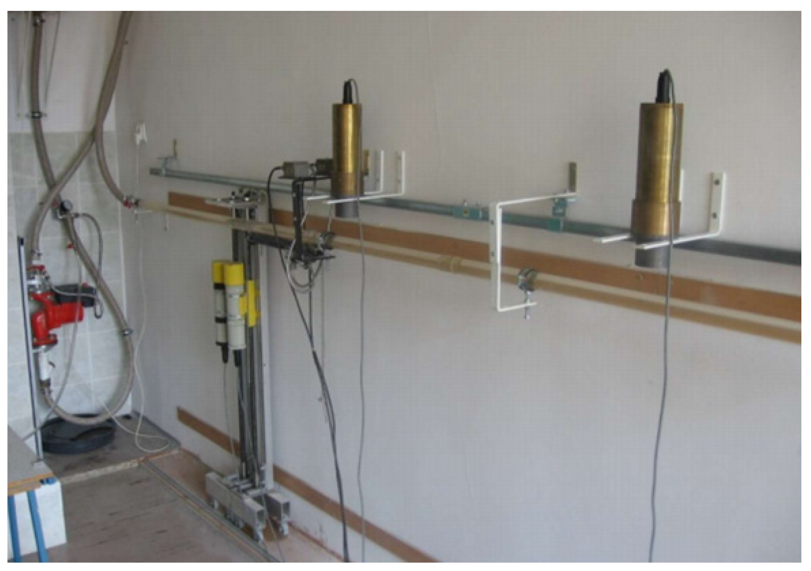
3. Experimental Setup

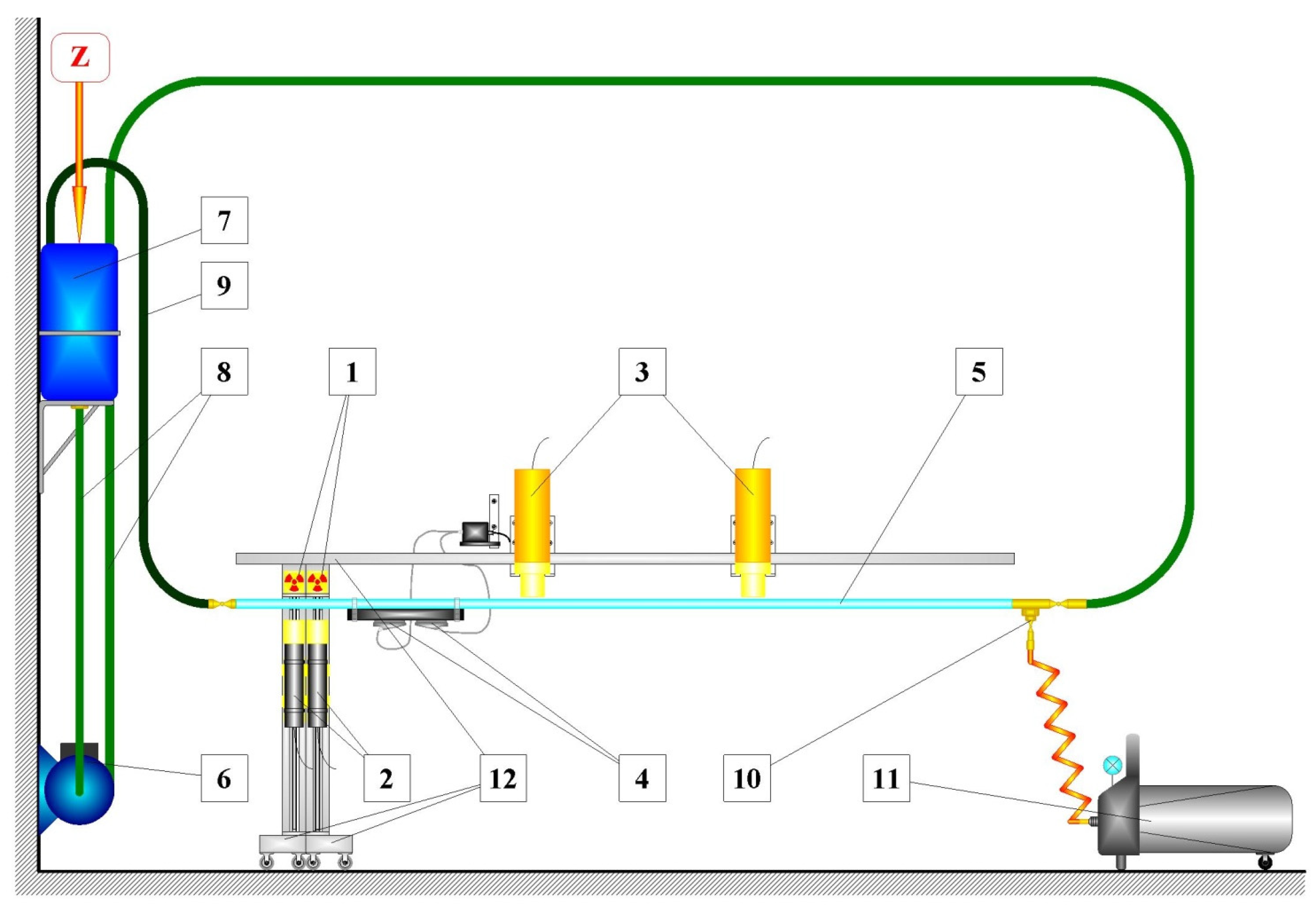
A general view of the experimental hydraulic installation is shown in Figure 2. This installation was built at the AGH University of Science and Technology in Kraków. A scheme of the laboratory set-up is introduced in Figure 3.

The hydraulic system is a closed circuit with a venting tank (7), which also forms a liquid expansion container. Water flow is achieved using a pump (6) controlled by an inverter. The pump speed control range is 1000–2800 rpm, which corresponds to velocity range of the flow from 0.5 m/s to 3.6 m/s. The measuring section of the pipeline (5) is a transparent Plexiglas pipe, length 4.5 m and internal diameter 30 mm, which is connected to the pump and the expansion-venting tank using flexible reinforced pipes (8, 9). The transparent section of the pipe allows the recording of a gas phase image using a fast camera. In addition, it is possible to mount ultrasonic probes (4) directly in the measuring section of the pipeline. Air from compressor (11) is forced into the initial part of the measuring section of the pipeline through a nozzle (10). The shifting system (12) with a rail guide is used to mount the absorption sets. The carts are equipped with tables with holes for source collimators (1) and clamps for gamma radiation detectors (2). The sliding system enables the distance between the detector and the radiation source to be changed by means of a lead screw and to change the distance between the sets.

In the experiments two gamma-ray sources ²⁴¹Am were used emitting photons with 59.5 keV energy, and detectors with NaI(Tl) 2″ scintillation crystals.

The stand shown in Figure 3 also allows for testing of flows using the tracer method. Measurements by means of radioactive markers are possible thanks to the fixed catches for the probes together with collimators (3) and the possibility of introducing radioactive solutions through the vent hole in the expansion tank (the marker feed site is marked Z in Figure 3). The test stand also includes a DAQ system, a PC with software that enables the analysis of signals from probes, and an ultrasonic flow meter to measure the velocity of the liquid. The DAQ module and software are used to allow data acquisition with an adjustable sampling time Δt from 0.1 ms, and the typical measurement time required to collect a representative number of data is 3–8 min.

4. Analysis of Measured Signals

The impulse waveforms I_x(t) and I_y(t) received from the probes counted at a specific sampling time Δt create discrete stochastic measuring signals x(n) and y(n). Examples of such signals (first 10,000 samples, after centring) obtained in the LIW experiments for four types of flow types as the bubble, plug-bubble, plug, and slug are shown in

Table 1. Examples of flow structures and signals x(n) obtained in LIW1, LIW2, LIW4, and LIW5 experiments.

Experiment	Example of Flow Structure	Signal x(n)
LIW1 bubble flow
LIW2 transitional plug–bubble flow
LIW4 plug flow
LIW5 slug flow

. The signal bandwidth was below 100 Hz, the sampling frequency 1 kHz (Δt = 1 ms), and the recorded data blocks counted N = 480,000 samples (8 min of measurement). The waveforms in the Table 1 require filtering before further analysis to remove radiation background noise and interference from fluctuations of nuclear decay [22]. This was accomplished using appropriate pass-band digital filters. A correspondingly long collection of such signals can be considered ergodic and can be resolved in the time and frequency domain by various statistical methods [16,23,24].

Table 2. Basic parameters of flows for the analyzed experiments: υ_L—water velocity, Re—Reynolds number, α—void fraction.

Experiment	υL (m/s)	Re (-)	α (-)
LIW1	3.56	4.7 × 104	0.227
LIW2	3.28	4.3 × 104	0.240
LIW4	2.92	3.7 × 104	0.266
LIW5	1.66	1.9 × 104	0.434

summarizes the basic parameters of the analyzed flows from Table 1.

The Reynolds number Re was calculated from the equation [25]:

$$\mathit{Re}=\frac{{\upsilon }_{L }·D_{\mathit{ch}}·\rho }{\eta }$$

(2)

where ρ is the density of the liquid, η is the dynamic viscosity, and D_ch is the characteristic dimension for the liquid phase, defined for the pipeline with inner radius r, as [25]:

$$D_{\mathit{ch}}=r\sqrt{1 - \alpha }$$

(3)

Void fraction α is defined as follows:

$$\alpha =\frac{V_G}{V_{}}$$

(4)

where V_G is the volume of air, and V is the total volume of medium in the pipe.

In the absorption method, a γ ray beam passes through the cross-section of the pipeline. For this cross-section, Equation (4) can be replaced by the formula [9]:

$$\alpha =\frac{A_G}{A}$$

(5)

where A_G is the surface area taken up by gas, and A is the surface area of the internal cross-section of the pipe.

4.1. Cross-Correlation Method

The cross-correlation method has been known and used for many years in signal analysis [16,17]. The discrete estimator of the CCF can be calculated from the relationship:

$${\widehat{R}}_{CCF}(k)=\frac{1}{N}{\displaystyle \sum _{n=0}^{N-1}x(n)y(n+k)}\hspace{1em}\hspace{1em}k=0,\hspace{0.17em}1,\hspace{0.17em}2\dots K$$

(6)

where N is the number of samples, k is the discrete value of the transportation time delay k = τ/Δt, and K is the number of function values.

The transportation time delay is designated as the argument of the main maximum CCF [16]. An example of the CCF in the LIW experiments is presented in Figure 4.

4.2. Differential Methods

Discrete estimators of the AMDF and ASDF differential functions can be presented by the following equations [24,26]:

$${\widehat{R}}_{AMDF}(k)=\frac{1}{N}{\displaystyle \sum _{n=0}^{N-1}\left|x(n)-y(n+k)\right|}\hspace{1em}\hspace{1em}k=0,\hspace{0.17em}1,\hspace{0.17em}2\dots K$$

(7)

$${\widehat{R}}_{ASDF}(k)=\frac{1}{N}{{\displaystyle \sum _{n=0}^{N-1}\left[x(n)-y(n+k)\right]}}^2\hspace{1em}\hspace{1em}k=0,\hspace{0.17em}1,\hspace{0.17em}2\dots K$$

(8)

In both differential functions, the transportation time delay can be designated as the location of the main minimum of functions (7) and (8). Simulation studies of differential methods AMDF and ASDF were presented in the work [18].

4.3. Combined Methods

Good metrological properties can be obtained by using combined methods for the analysis of stochastic signals from scintillation detectors, such as a quotient of CCF and ASDF and AMDF differential functions according to the formulas:

$${\widehat{R}}_{CCF/AMDF}(k)=\frac{{\widehat{R}}_{CCF}(k)}{{\widehat{R}}_{AMDF}(k)}\hspace{1em}\hspace{1em}k=0,\hspace{0.17em}1,\hspace{0.17em}2\dots K$$

(9)

$${\widehat{R}}_{CCF/ASDF}(k)=\frac{{\widehat{R}}_{CCF}(k)}{{\widehat{R}}_{ASDF}(k)}\hspace{1em}\hspace{1em}k=0,\hspace{0.17em}1,\hspace{0.17em}2\dots K$$

(10)

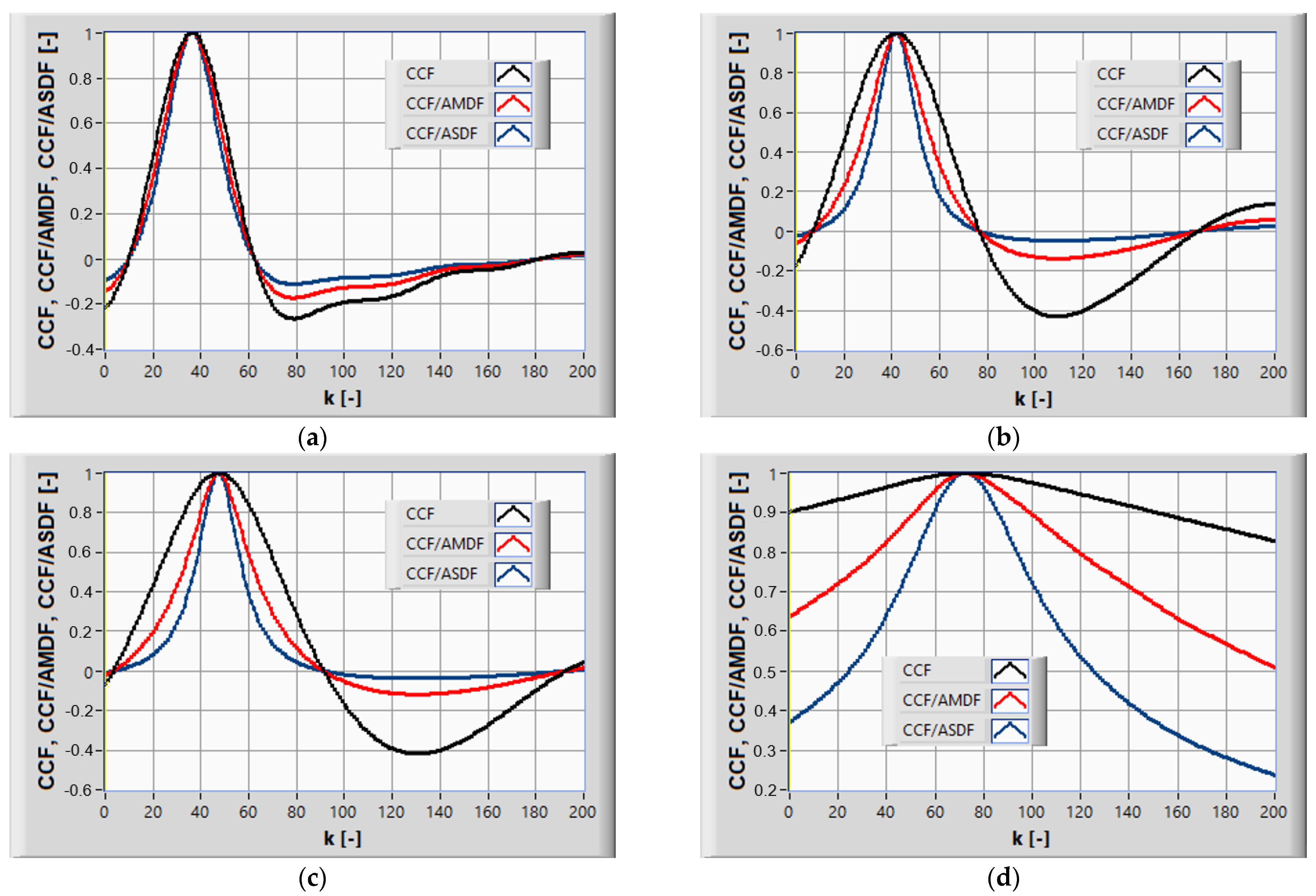
The use of functions (9) and (10) to analyse the signals registered in the LIW experiments allows us to obtain the waveforms shown in Figure 4. Figure 4 shows the functions normalized to the maximum values, CCF was normalized similarly. Due to this, it is easy to see that the obtained CCF/ASDF and CCF/AMDF waveforms have a slightly higher steepness in the vicinity of the extreme points than the CCF.

5. Measurement Results

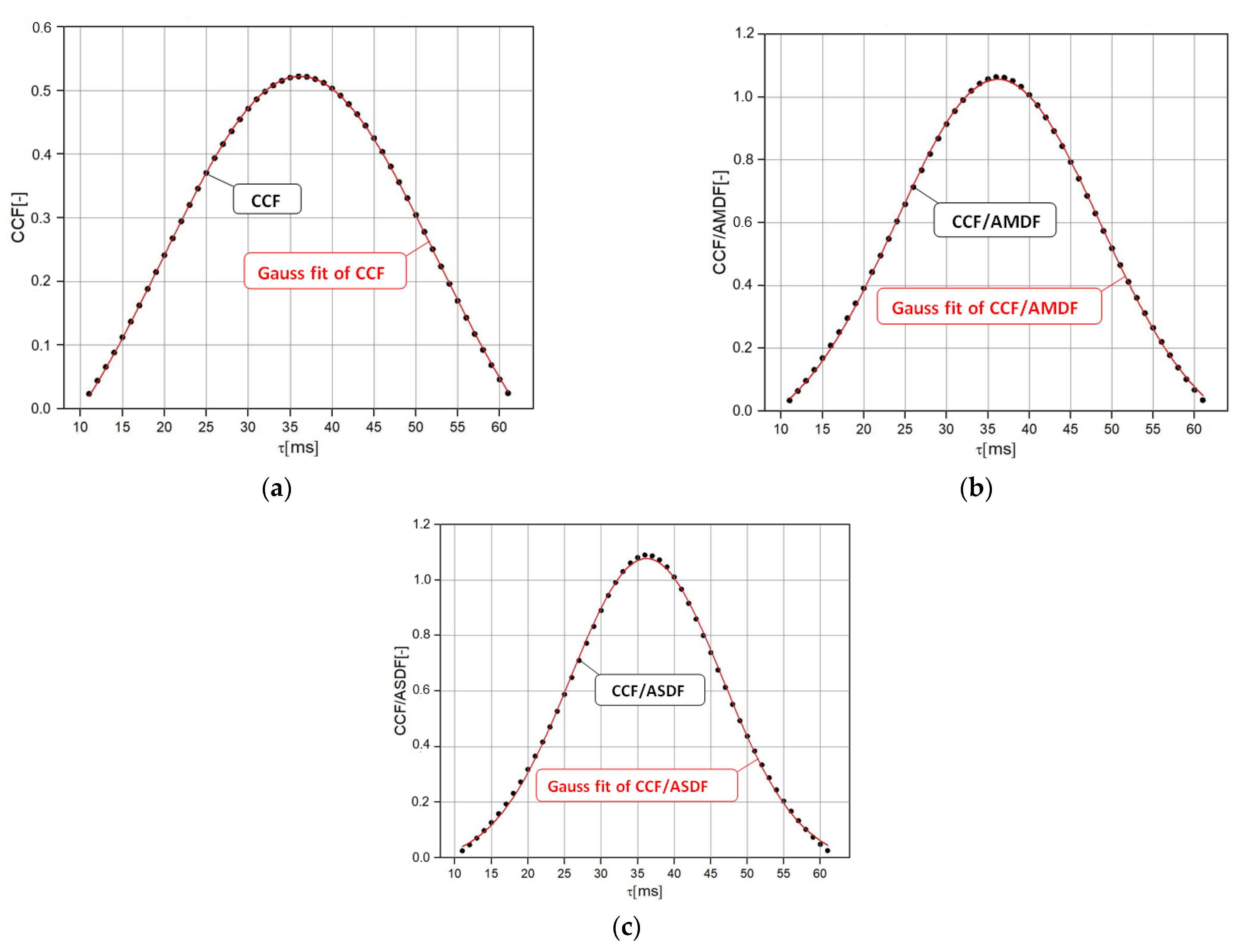
For all waveforms presented in Figure 4, the procedure for designating the location of the main extreme was used, consisting of the interpolation of the selected fragment of obtained characteristics with the Gauss function (in each case the same number of points was used):

$$p\left(\tau \right)=p_0+\frac{1}{\sigma \sqrt{2\pi }}\exp \left(-\frac{{\left(\tau -{\widehat{\tau }}_0\right)}^2}{2{\sigma }^2}\right)$$

(11)

where p₀ is the normalization level of the Gauss function and σ is the standard deviation of its distribution.

The samples of Gauss fit results for the characteristics CCF, CCF/AMDF, and CCF/ASDF obtained in the LIW 1 run are presented in Figure 5. In this case, the transportation time delay estimator ${\widehat{\tau }}_0$ is designated as the first moment of the matched distribution. The standard uncertainty of the time delay $u\left({\widehat{\tau }}_0\right)$ can be determined from the equation [18]:

$$u\left({\widehat{\tau }}_0\right)=\frac{\sigma }{\sqrt{m}}$$

(12)

where m is the number of points used in the interpolation procedure (m = 51 for all cases).

The average velocity of the dispersed phase υ_G (air bubbles) can be calculated from Formula (1). With negligibly small uncertainties in the measurement path, the combined standard uncertainty u_c(υ_G) depends on the inaccuracy of determining the uncorrelated quantities L and ${\widehat{\tau }}_0$:

$$u_c({\upsilon }_G)=\sqrt{{\left(\frac{\partial {\upsilon }_G}{\partial L}\right)}^2{u}_B{}^2(L)+{\left(\frac{\partial {\upsilon }_G}{\partial {\widehat{\tau }}_0}\right)}^2{u}_A{}^2({\widehat{\tau }}_0)}$$

(13)

where u_B(L) is the standard uncertainty of measuring the distance between probes (u_B(L) = 0.02 mm), and u_A(${\widehat{\tau }}_0$) is the standard uncertainty in determining the average transportation time delay. Indexes A and B mean, respectively, uncertainty type A and type B [27,28].

Expanded uncertainty U_0.95(υ_G) was calculated from dependence:

U_0.95(υ_G) = k_p u_c(υ_G)

(14)

where k_p is the coverage factor (k_p = 2 was adopted).

The results of the measurements of the average velocity υ_G and the expanded uncertainties U_0.95(υ_G) obtained in the LIW experiments are summarized in

Table 3. The results of measurements obtained in the LIW experiments.

Experiment	Method	${\widehat{\mathsf{\tau }}}_{\mathbf{0}}\mathbf{\left(}\mathit{m}\mathit{s}\mathbf{\right)}$	$\mathsf{\sigma }\mathbf{\left(}\mathit{m}\mathit{s}\mathbf{\right)}$	$\mathit{u}\mathbf{\left(}{\widehat{\mathsf{\tau }}}_{\mathbf{0}}\mathbf{\right)}\mathbf{\left(}\mathit{m}\mathit{s}\mathbf{\right)}$	${\mathsf{\upsilon }}_{\mathit{G}}\mathbf{\left[}\frac{\mathit{m}}{\mathit{s}}\mathbf{\right]}$	${\mathit{U}}_{\mathbf{0.95}}\mathbf{\left(}{\mathsf{\upsilon }}_{\mathit{G}}\mathbf{\right)}\mathbf{\left[}\frac{\mathit{m}}{\mathit{s}}\mathbf{\right]}$	${\mathit{R}}^{\mathbf{2}}\mathbf{[}\mathbf{-}\mathbf{]}$
LIW1	CCF	36.21	16.43	2.30	2.68	0.34	0.99998
	CCF/AMDF	36.24	11.22	1.57	2.68	0.23	0.99996
	CCF/ASDF	36.22	9.34	1.31	2.68	0.24	0.99993
LIW2	CCF	41.80	22.61	3.17	2.32	0.35	1.00000
	CCF/AMDF	41.82	9.55	1.34	2.32	0.15	0.99759
	CCF/ASDF	41.80	6.96	0.98	2.32	0.11	0.99620
LIW4	CCF	47.31	22.61	3.17	2.05	0.27	0.99999
	CCF/AMDF	47.29	9.55	1.34	2.05	0.12	0.99876
	CCF/ASDF	47.30	6.96	0.98	2.05	0.08	0.99938
LIW5	CCF	72.86	28.37	3.97	1.33	0.15	0.99917
	CCF/AMDF	73.02	22.90	3.21	1.33	0.12	0.98822
	CCF/ASDF	72.83	17.45	2.44	1.33	0.09	0.99921

. The R² parameter means the determination coefficient.

Table 4. The values of relative uncertainty $U_{0.95}{\left({\upsilon }_G\right)}_{rel}$.

Experiment	Method	$${\mathit{U}}_{0.95}{\left({\mathit{\upsilon }}_{\mathit{G}}\right)}_{\mathit{r}\mathit{e}\mathit{l}}\left(\mathit{\%}\right)$$
LIW1	CCF	100
	CCF/AMDF	68
	CCF/ASDF	57
LIW2	CCF	100
	CCF/AMDF	42
	CCF/ASDF	31
LIW4	CCF	100
	CCF/AMDF	42
	CCF/ASDF	31
LIW5	CCF	100
	CCF/AMDF	80
	CCF/ASDF	62

shows the relative uncertainty values $U_{0.95}{\left({\upsilon }_G\right)}_{rel}$ relative to the uncertainty values for CCF. As can be seen, in each case the uncertainties for the combined methods CCF/ASDF and CCF/AMDF are smaller than for the cross-correlation.

6. Conclusions

This article presents an example of the application of the gamma absorption method to measure the dispersed phase velocity of a two-phase water–air flow in a horizontal pipe. In addition to the classical cross-correlation function, the analysis of signals from scintillation probes uses the relatively less popular methods, AMDF and ASDF, which allow obtaining combined methods: CCF/ASDF and CCF/AMDF.

As shown in Figure 4, the combined functions have a steeper course in the vicinity of the extreme point than the CCF. Comparison of the measurement results obtained for the four flow structures as the bubble, transitional plug-bubble, plug, and slug flows shows that the smallest values of the uncertainty of all measurements of average air bubble velocity were obtained in order for methods: CCF/ASDF, CCF/AMDF, and CCF. For CCF/AMDF, the uncertainty $U_{0.95}{\left({\upsilon }_G\right)}_{rel}$ is from 42% to 80% of the uncertainty for cross-correlation. For the CCF/ASDF method, it is from 31% to 62%, respectively. The results obtained confirm the universality of the described methods for the experimental conditions obtained. In two-phase flows, the velocity of movement of individual bubbles in a swarm of bubbles is different and depends on many parameters. Therefore, the obtained uncertainties undoubtedly contain deviations resulting from the natural movement of gas bubbles and do not reflect only the uncertainty of the measurement method.

References

- Mohamad, E.J.; Rahim, R.A.; Rahiman, M.H.F.; Ameran, H.L.M.; Muji, S.Z.M.; Marwah, O.M.F. Measurement and analysis of water/oil multiphase flow using electrical capacitance tomography sensor. Flow Meas. Instrum. 2016, 47, 62–70. [Google Scholar] [CrossRef]
- Rahim, R.A.; Yunos, Y.M.; Rahiman, M.H.F.; Muji, S.Z.M.; Thiam, C.K.; Rahim, H.A. Optical tomography: Velocity profile measurement using orthogonal and rectilinear arrangements. Flow Meas. Instrum. 2012, 23, 49–55. [Google Scholar] [CrossRef]
- Rzasa, M.R.; Plaskowski, A. Application of optical tomography for measurements of aeration parameters in large water tanks. Meas. Sci. Technol. 2003, 14, 199–204. [Google Scholar] [CrossRef]
- Heindel, T.J.; Gray, J.N.; Jensen, T.C. An X-ray system for visualizing fluid flows. Flow Meas. Instrum. 2008, 19, 67–78. [Google Scholar] [CrossRef]
- Lindken, R.; Merzkirch, W. A novel PIV technique for measurements in multiphase flows and its application to two-phase bubbly flows. Exp. Fluids 2002, 33, 814–825. [Google Scholar] [CrossRef]
- Lamadie, F.; Charton, S.; de Langlard, M.; Ouattara, M.; Sentis, M.P.; Debayle, J.; Onofri, F.R. Development of optical techniques for multiphase flows characterization. In Proceedings of the ASME 2017 Fluids Engineering Division Summer Meeting, Waikoloa, HI, USA, 30 July–3 August 2017. [Google Scholar] [CrossRef]
- Tamburini, A.; Cipollina, A.; Micale, G.; Brucato, A. Particle distribution in dilute solid liquid unbaffled tanks via a novel laser sheet and image analysis based technique. Chem. Eng. Sci. 2013, 87, 341–358. [Google Scholar] [CrossRef]
- Johansen, G.A.; Jackson, P. Radioisotope Gauges for Industrial Process Measurements; John Wiley: New York, NY, USA, 2004. [Google Scholar]
- Zych, M.; Hanus, R.; Jaszczur, M.; Strzępowicz, A.; Petryka, L.; Mastej, W. Determination of void fraction in two phase liquid-gas flow using gamma absorption. J. Phys. Conf. Ser. 2016, 745, 032124. [Google Scholar] [CrossRef]
- Mosorov, V. Improving the accuracy of single radioactive particle technique for flow velocity measurements. Flow Meas. Instrum. 2019, 66, 150–156. [Google Scholar] [CrossRef]
- Karami, A.; Roshani, G.H.; Khazaei, A.; Nazemi, E.; Fallahi, M. Investigation of different sources in order to optimize the nuclear metering system of gas–oil–water annular flows. Neural Comput. Appl. 2020, 32, 3619–3631. [Google Scholar] [CrossRef]
- Salgado, W.; Dam, R.; Salgado, C. Optimization of a flow regime identification system and prediction of volume fractions in three-phase systems using gamma-rays and artificial neural network. Appl. Radiat. Isot. 2021, 169, 109552. [Google Scholar] [CrossRef]
- Roshani, M.; Phan, G.; Faraj, R.H.; Phan, N.-H.; Roshani, G.H.; Nazemi, B.; Corniani, E.; Nazemi, E. Proposing a gamma radiation based intelligent system for simultaneous analyzing and detecting type and amount of petroleum by-products. Nucl. Eng. Technol. 2021, 53, 1277–1283. [Google Scholar] [CrossRef]
- Krupička, J.; Matousek, V. Gamma-ray-based measurement of concentration distribution in pipe flow of settling slurry: Vertical profiles and tomographic maps. J. Hydrol. Hydromech. 2014, 62, 126–132. [Google Scholar] [CrossRef]
- Rząsa, M.R. Comparison of selected theoretical models of bubble formation and experimental results. Arch. Thermodyn. 2014, 35, 21–36. [Google Scholar] [CrossRef]
- Beck, M.S.; Pląskowski, A. Cross-Correlation Flowmeters; Adam Hilger: Bristol, UK, 1987. [Google Scholar]
- Jung, S.-H.; Kim, J.-S.; Kim, J.-B.; Kwon, T.-Y. Flow-rate measurements of a dual-phase pipe flow by cross-correlation technique of transmitted radiation signals. Appl. Radiat. Isot. 2009, 67, 1254–1258. [Google Scholar] [CrossRef]
- Hanus, R.; Zych, M.; Petryka, L.; Świsulski, D. Time delay estimation in two-phase flow investigation using the γ-ray attenuation technique. Math. Probl. Eng. 2014, 2014, 475735. [Google Scholar] [CrossRef]
- Hanus, R.; Petryka, L.; Zych, M. Velocity measurement of the liquid–solid flow in a vertical pipeline using gamma-ray absorption and weighted cross-correlation. Flow Meas. Instrum. 2014, 40, 58–63. [Google Scholar] [CrossRef]
- Hanus, R.; Zych, M.; Petryka, L. Differential and combined methods of signal analysis in radioisotope measurements of dispersed phase velocity in a liquid-gas flow through a horizontal pipeline. Prz. Elektrotech. 2015, 90, 60–63. (In Polish) [Google Scholar]
- Hanus, R.; Zych, M.; Petryka, L. Velocity measurement of two-phase liquid-gas flow in a horizontal pipeline using gamma densitometry. J. Phys. Conf. Ser. 2014, 530, 012042. [Google Scholar] [CrossRef]
- Zych, M.; Hanus, R.; Wilk, B.; Petryka, L.; Świsulski, D. Comparison of noise reduction methods in radiometric correlation measurements of two-phase liquid-gas flows. Measurement 2018, 129, 288–295. [Google Scholar] [CrossRef]
- Bendat, J.S.; Piersol, A.G. Random Data—Analysis and Measurement Procedures, 4th ed.; John Wiley: New York, NY, USA, 2010. [Google Scholar]
- Jacovitti, G.; Scarano, G. Discrete time technique for time delay estimation. IEEE Trans. Signal Process. 1993, 41, 525–533. [Google Scholar] [CrossRef]
- Morgado, A.; Miranda, J.; Araújo, J.; Campos, J. Campos, Review on vertical gas–liquid slug flow. Int. J. Multiph. Flow 2016, 85, 348–368. [Google Scholar] [CrossRef]
- Chen, J.; Benesty, J.; Huang, Y. Performance of GCC- and AMDF-based time-delay estimation in practical reverberant environments. EURASIP J. Adv. Signal Process. 2005, 2005, 498964. [Google Scholar] [CrossRef]
- Joint Committee for Guides in Metrology (JCGM). Guide to the Expression of Uncertainty in Measurement; Joint Committee for Guides in Metrology (JCGM): Sèvres, French, 2008; p. 100. [Google Scholar]
- The American Society of Mechanical Engineers. Guidelines for the Evaluation of Dimensional Measurement Uncertainty; ASME B89.7.3.2-2007 (R2011); American National Standards Institute (ANSI): New York, NY, USA, 2007. [Google Scholar]