Optimization of Load Sharing in Compressor Station Based on Improved Salp Swarm Algorithm

Abstract

In long-distance gas transmission pipelines, there are many booster compressor stations consisting of parallel compressors that provide pressure for the delivery of natural gas. So, it is economically important to optimize the operation of the booster compressor station. The booster compressor station optimization problem is a typical mixed integer nonlinear programming (MINLP) problem, and solving it accurately and stably is a challenge. In this paper, we propose an improved salp swarm algorithm based on good point set, adaptive population division and adaptive inertia weight (GASSA) to solve this problem. In GASSA, three improvement strategies are utilized to enhance the global search capability of the algorithm and help the algorithm jump out of the local optimum. We also propose a constraint handling approach. By using semi-continuous variables, we directly describe the on or off state of the compressor instead of using auxiliary binary variables to reduce the number of variables and the difficulty of solving. The effectiveness of GASSA is firstly verified using eight standard benchmark functions, and the results show that GASSA has better performance than other selected algorithms. Then, GASSA is applied to optimize the booster compressor station load distribution model and compared with some well-known meta-heuristic algorithms. The results show that GASSA outperforms other algorithms in terms of accuracy and reliability.

1. Introduction

In the transportation of oil and gas, the common means of transportation are road, rail, water, air and pipeline [1]. Pipelines are indispensable in oil and gas transportation because they are a safer [2], greener [3] and more economical [4] means of transportation than other means of transportation. With the continuous development of society and economy, the demand for petrochemical products has been increasing in all industries, especially the demand for natural gas has increased dramatically [5]. As a result, a large number of natural gas pipelines are being built and grouped all over the world [6], and pipelines have been expanding all over the world.

With larger pipe diameters in long gas transmission pipelines, the pressure of natural gas drops significantly as it flows due to friction and heat transfer [7]. In addition, there is a minimum demand for natural gas pressure from natural gas customers [8]. In order to increase the natural gas pressure, natural gas pipeline companies often build a large quantity of booster compressor stations in long gas transmission pipelines [9], where multiple compressors are usually connected in parallel. The energy consumption of the compressor station accounts for a significant proportion of the company’s operating costs. Due to its huge economic impact, the optimal operation of the booster compressor station becomes very important [10]. The compressors are usually driven by variable frequency electric drives or variable frequency gas turbines, and the power provided by the compressors varies with the gas flow rate and inlet conditions [11]. The manager of the booster compressor station needs to decide on the working compressor units, the speed of the working compressor units and the sharing of natural gas flows between the compressor units [12]. In actual scheduling, the manager determines the number of units to be started based on experience, and the flow rate among the units is evenly divided. Load sharing optimization is to minimize power consumption at the booster compressor station by redistributing the flow rate among the units and reselecting the working compressor groups and the compressor speed. A traditional operation problem is thus formed, i.e., minimizing the total power of all compressors under the working domain constraint and the flow balance constraint [13]. The working domain constraint means that there should be a certain relationship between the physical characteristics such as the polytropic head, polytropic efficiency, compression ratio and volume flow rate. The flow balance constraint is that the total flow through the compressors is balanced by the total flow at the booster compressor station.

The optimization of the booster compressor station has been considered in recent years of research. Regarding the research on the optimal operation of the booster compressor station, some scholars have approached this problem by classical mathematical methods. Specifically, Deng [12] compared the results of mixed integer linear and dynamic programming (DP) solutions for different volume flow dispersion intervals. Milosavljevic et al. [14] used real-time optimization techniques (RTO) to optimize the compressor load distribution, but they did not take into account the on/off state of the compressor. Cortinovis et al. [15] used historical data to update the performance model of the compressor and selected working compressors by performance tracking instead of binary variables. Zapukhliak et al. [16] considered a special case in the gas transmission pipeline, when the main transmission system is underloaded, using a mathematical model to estimate the pressure variations along its length in the gas pipeline.

However, meta-heuristic algorithms present effectiveness and ease of implementation in solving various types of complex engineering optimization problems. This has led researchers to propose many meta-heuristic algorithms for optimal operation of the booster compressor station. For example, Liu et al. [17] developed a combined air cooler and compressor operation model and optimized the model using the genetic algorithm (GA), particle swarm algorithm (PSO) and simulated annealing (SA) algorithm. Division et al. [18] considered a new load distribution model and optimized the model using a hybrid algorithm of crow search algorithm (CSA) and symbiotic organisms search (SOS). Regarding current newer technology, Li et al. [19] eliminated binary variables by reformulating MINLP to reduce the difficulty of optimization and optimized the reformulated model using a hybrid algorithm of differential evolution (DE) and whale optimization algorithm (WOA). Combining the above references, the research on the optimal operation of booster compressor station focuses on the construction and simplification of the booster compressor station model on the one hand and the improvement and application of the meta-heuristic algorithm on the other hand, which is a very important guideline for the optimization of the booster compressor station model in this paper.

The Salp Swarm Algorithm (SSA), which simulates the living and eating behaviors of salp swarm, was developed by Mirjalili et al. in 2017 [20]. Its mathematical model may be divided into two groups: one group is the leader and the other group is the follower. The first member in the chain is the leader, and the rest of the members are the followers. In the algorithm, the leader leads the population to find the optimal food, and the followers follow the nearest bottle sheaths. In addition, its simple structure and few control parameters have led to it becoming a popular research area in the field of algorithms, attracting many scholars to study and apply it in different fields, such as controller parameter optimization [21], power tracking of photovoltaic systems [22] and soil retention evaluation [23]. These reflect the outstanding performance of SSA in some fields and prove the high flexibility and reliability of the method. Although the SSA has shown outstanding performance in many fields, it still has many challenging problems, such as slow convergence and easily falling into localization during the iterative process.

Based on a comprehensive review of the literature, it is found that standard SSA and its variants have not been used to optimize the booster compressor station. The aim of this work is to propose a promising novel method that can accurately and reliably optimize the booster compressor station model to reduce the cost of energy consumption in the booster compressor station. Therefore, an improved SSA is proposed for optimizing the load distribution model of the booster compressor station. The main contributions of this paper are as follows.

1. Semi-continuous variables are used to describe the operating state of the compressor, and effective constraint handling methods are used to solve the domain holes that appear after using semi-continuous variables.

2. To propose an improved version of SSA (GASSA) for the optimization problem of the booster compressor station model.

3. Adding good point set initialization, adaptive population division and adaptive inertia weight to address the shortcomings of the standard SSA. Using eight benchmark test functions and a booster compressor station load sharing model to verify the effectiveness of GASSA.

The rest of the paper is organized as follows: Section 2 provides the MINLP mathematical model for the load-sharing problem at the booster compressor station. Section 3 describes the model preprocessing methods, standard SSA and GASSA implementations. Section 4 provides the benchmark test functions and the load-sharing model optimization results. Finally, Section 5 gives the conclusions of this paper.

2. Model

2.1. Object Function

Based on the current configuration of compressor units in most gas transmission pipeline compressor stations, we considers a compressor station configured with multiple parallel electrically driven centrifugal compressor units. Figure 1 shows a schematic diagram of parallel compressor uints, the compressor uint has three components: drive, compressor and cooler. The natural gas passing through the compressor is very hot and needs to be cooled by the cooler before it can be transported. The power consumption of the cooler is much smaller than the power consumption consumed by the compressor, so the power consumption of the cooler is not considered. The objective function considered here is to minimize the power consumption of the electric drive compressor.

$$P=min\sum _{i=1}^n{P}_{iN}$$

(1)

where P is the total energy consumption of the compressor station $\left(\mathrm{MW}\right)$, $P_{iN}$ is the energy consumption of the $i^{th}$ compressor $\left(\mathrm{MW}\right)$ and n is the number of compressors in the station.

2.2. Constraints

2.2.1. Compressor Unit Limitations

We discusses the mathematical calculations of compressor power and working domain that are accepted and used by most people [24], as shown below.

The movement of the gas through the compressor is a polytropic process. Once operating parameters are given, such as compression ratio, temperature, etc., the following equation [11] can be used to calculate the polytropic head H$(\mathrm{J}/\mathrm{kg})$.

$$H=\frac{Z_s·R·T_s}{(\sigma -1)/\sigma }\left[{\epsilon }^{\sigma -1/\sigma }-1\right]$$

(2)

where $Z_s$ is the compression factor on the suction side of the compressor, R is the gas constant $(\mathrm{J}/\mathrm{kg}·\mathrm{K})$, $T_s$ is the temperature on the suction side of the compressor $\left(\mathrm{K}\right)$, $\sigma$ is the isentropic exponent, and $\epsilon$ is the compression ratio. Similarly, the polytropic head can be expressed as a function of the compressor speed N and the gas flow rate Q [25].

$$H=b_1{N}^2+b_{2}NQ+b_3{Q}^2$$

(3)

where $b_1$, $b_2$ and $b_3$ are constants, N is the speed of the compressor $\left(\mathrm{rmp}\right)$, and Q is the volumetric flow rate of natural gas at the compressor inlet $({\mathrm{m}}^3/\mathrm{s})$. Based on the above two polytropic head equations, the head H can be calculated from the given suction conditions, compression ratio, and thus the speed N as a function of flow rate Q. Combining the two equations of the polytropic head, it is possible to obtain the speed N as a function of the volume flow Q according to the given operating parameters.

The operating domain range of the compressor is usually shown in Figure 2, which contains four boundaries [19]. In Figure 2, the upper and lower curves of the working domain correspond to the operating conditions at the maximum speed $N_{max}$ and the minimum speed $N_{min}$$\left(\mathrm{rmp}\right)$, respectively. Therefore, the operating speed of the compressor must satisfy the following equation [26].

$$N_{min}\le N\le N_{max}$$

(4)

In addition to speed limitations, the compressor capacity is limited by two instabilities (i.e., surge and stonewell). The surge line is expressed as [27].

$$Q_{surge}=a_1+a_{2}N+a_3{N}^2$$

(5)

where $a_1$, $a_2$ and $a_3$ are constants and $Q_{surge}$ is the minimum volume flow rate determined by the surge $({\mathrm{m}}^3/\mathrm{s})$.

The stonewell line can be calculated by the following equation [11].

$$Q_{stonewell}=a_4+a_{5}N+a_6{N}^2$$

(6)

where $a_4$, $a_5$ and $a_6$ are constants and $Q_{stonewell}$ is the maximum volume flow rate $({\mathrm{m}}^3/\mathrm{s})$.

Finally, the following equation [28] can be used to estimate the power consumption $P_N$ of the compressor $\left(\mathrm{MW}\right)$.

$$P_N=\frac{mH}{\eta }$$

(7)

where m is the mass flow rate of natural gas $(\mathrm{kg}/\mathrm{s})$ and $\eta$ is the polytropic efficiency.

Here, the mass flow rate m can be converted into the volume flow rate Q using the following equation.

$$Q=\frac{m·Z_s·R·T_s}{p_s}$$

(8)

where $p_s$ is the suction pressure of the compressor $\left(\mathrm{MPa}\right)$.

Equally, the polytropic efficiency can be expressed as a function of speed N and flow rate Q, as shown in the following equation.

$$\eta =b_4{N}^2+b_{5}NQ+b_6{Q}^2$$

(9)

where $b_4$, $b_5$ and $b_6$ are constants. Combining the efficiency equation and the mass flow conversion equation, power $P_N$ as a function of volume flow Q can be obtained for the given operating parameter, i.e., $P_N\left(Q\right)$.

2.2.2. Load Balance Constrainst

We have considered a compressor station with several parallel-connected compressors. For parallel compressors, the compression ratio must be the same, meaning that their suction conditions and discharge pressure should also be the same.

$${\epsilon }_i=u_i{\epsilon }_0$$

(10)

where ${\epsilon }_i$ is the compression ratio of the compressor station, and ${\epsilon }_0$ is the compressor ratio of the compressor. The on or off state of compressor i is indicated by introducing a binary variable $u_i$. When $u_i$ = 1, compressor i is in working state; when $u_i$ = 0, the compressor i is off.

At the same time, the volume flow rate via this compressor station ought to eventually be the same as the total volume flow rates through all of the individual compressors. $Q_0$ is the volume flow rate through the compressor station and $Q_i$ is the volume flow rate through compressor i.

$$\sum _{i=1}^n{u}_i{Q}_i=Q_0$$

(11)

To address the surge instability, it is common to have a recirculating bypass for each compressor, as shown in Figure 1. However, these flows are neglected in this load equation to avoid considering the surge instability. This simplification makes the equation simpler and does not alter the solution of the algorithm.

2.3. Question Summary

The model we considered is based on given operating parameters, such as suction pressure, temperature and compression ratio. Therefore, the polytropic head $H_0$ can be calculated based on the given parameters, as shown by the dashed line in Figure 2. Then, the range of the flow rate is calculated from the intersection of this line and the boundary line. In summary, the complete compressor station optimization model can be expressed as.

$$\begin{array}{c}min{\displaystyle \sum _{i=1}^n}{P}_{iN}\left(Q_i\right)\\ \mathrm{s}.\mathrm{t}.{\epsilon }_i=u_i{\epsilon }_0\\ {\displaystyle \sum _{i=1}^n}{u}_i{Q}_i=Q_0\\ u_i{Q}_{imin}\le Q_i\le u_i{Q}_{imax}\\ u_i\in \{0,1\}\\ \mathrm{for}i=1,2,\cdots n\end{array}$$

(12)

where $Q_{imin}$ and $Q_{imax}$ are the minimum and maximum flow rates, respectively.

3. Solution Approach

3.1. Model Preprocessing

In the above mathematical model, the objective function is nonlinear and contains a binary variable, so the issue is classified as a mixed integer nonlinear programming (MINLP) problem. For the given suction condition and compression ratio, the problem is governed by the flow balance constraint at the compressor station and the compressor operating domain. Most meta-heuristic algorithms are an unconstrained optimization algorithm and are based on continuous variable solving, so our model cannot be solved directly by meta-heuristic algorithms. In this case, we must perform constraint handling to transform it into an unconstrained optimization problem. We mainly consider the flow balance constraint and the binary variables that indicate the on or off state of the compressor.

3.1.1. Binary and Semi-Continuous Variables

The binary variable is an auxiliary variable to represent the on or off state of the compressor; here, we use a more concise strategy to express the state of the compressor [29,30], i.e., semi-continuous variables. Before discussing why the binary variable is discarded, we briefly describe the connection between the binary and semi-continuous variables in unit optimization. In Equation (12), if a unit is on, i.e., $u_i$ = 1, the flow through this compressor is within $[Q_{imin}$,$Q_{imax}]$; otherwise, $u_i$ = 0 and the flow through is 0. With this approach, the binary variable represents whether the unit is on or off. We can also consider the flow $Q_i$ to determine the on or off state of the unit alone. When $Q_i$ belongs to $[Q_{imin},Q_{imax}]$, the unit is in the on state. When $Q_i$ = 0, the unit is in the off state. As mentioned above, $Q_i$ is the semi-continuous variable that takes values in the range $0\cup [Q_{imin},Q_{imax}]$.

Figure 3 further illustrates the difference between binary and semi-continuous variables. For example, if $Q_{min}$ = 1 and $Q_{max}$ = 5, we have u = 0.8 and Q = 4 at this time. Since u is not an integer, we need to further integerize u. We can see that the introduction of binary variables increases the difficulty of solving the model, while the use of semi-continuous variables greatly simplifies the problem model. So, we do not use binary variables and reuse semi-continuous variables to construct the whole problem model.

From the above, it is clear that there is a domain hole constraint for semi-continuous variables (i.e., it cannot equal the value greater than 0 but less than $Q_{imin}$). In the meta-heuristic algorithm designed primarily for unconstrained optimization problems, the constraint can be treated either explicitly or implicitly. For each domain hole in the model, we use an implicit constraint treatment to satisfy the domain hole constraint. In the implicit processing strategy, the algorithm itself is modified by performing some additional operations on the group members to ensure that the members satisfy the constraints. To be specific, if the unit is on, the flow rate should be between $[Q_{imin},Q_{imax}]$. If $Q_i$ is bigger than 0 and less than $Q_{imin}$, the unit should not be turned on, i.e., the flow rate is 0, as shown below.

$$\left(Q_i>0\right)\&\left(Q_i<Q_{imin}\right)\Rightarrow Q_i=0;i=1,2,\cdots ,n$$

(13)

3.1.2. Flow Balance Constraint

To satisfy the flow balance constraint, the dynamic penalty function method is used to deal with the equation constraint [31]. To be specific, by establishing a new fitness function in place of the previous objective function, the new fitness function consists of two parts, i.e., the objective function and the penalty function. The new fitness function is as follows.

$$minFit=\sum _{i=1}^n{P}_{iN}+cl(\sum _{i=1}^n{Q}_i-Q_0)$$

(14)

where c is a constant, and l is the number of iterations. By using the smaller penalty factor at the beginning of the iteration, the penalty for infeasible solutions is smaller, so the algorithm will have the possibility to search beyond the feasible domain to some extent. However, using the bigger penalty function at the later stage makes the algorithm’s search focus on the feasible domain to find the better feasible solution.

3.2. Salp Swarm Algorithm

The salp swarm optimization algorithm is analogous to other meta-heuristic optimization algorithms. First, the populations are randomly initialized. The location vector X of the salp population is composed of N salp individuals of dimension D, as shown in Equation (15). The search space’s objective or food source is designated as F. Each leader’s position is changed in the direction of F, and the update equation is shown in Equation (16).   

$$\begin{array}{c}X=\left[\begin{array}{cccc}{x}_1^1& x_2^1& \cdots & x_D^1\\ x_1^2& x_2^2& \cdots & x_D^2\\ ⋮& ⋮& \ddots & ⋮\\ x_1^N& x_2^N& \cdots & x_D^N\end{array}\right]\end{array}$$

(15)

$$x_j^1=\left\{\begin{array}{c}{F}_j+c_1\left(\left(u{b}_j-l{b}_j\right)c_2+l{b}_j\right), c_2⩾0.5\hfill \\ F_j-c_1\left(\left(u{b}_j-l{b}_j\right)c_2+l{b}_j\right), c_3<0.5\hfill \end{array}\right.$$

(16)

where $x_j^1$ is the position of the first salp in dimension j, $F_j$ denotes the food position in dimension j, and $u{b}_j$ and $l{b}_j$ are the upper and lower bounds of the dimension, respectively. $c_2$ and $c_3$ are the random numbers within $\left[0,1\right]$, which are used to determine whether the leader’s next position should be in the positive or negative direction and the length of the move. $c_1$ is the important parameter in the leader position update formula; it is defined as follows.

$$\begin{array}{c}{c}_1=2{\mathrm{e}}^{-{\left(\frac{4l}{L_{\max }}\right)}^2}\end{array}$$

(17)

where l is the current number of iterations, and $L_{max}$ is the maximum number of iterations defined.

The movement of the follower is guided by the leader, and the follower position update formula is shown in Equation (18).

$$\begin{array}{c}{x}_j^i=\frac{1}{2}\left(x_j^i+x_j^{i-1}\right)\end{array}$$

(18)

where $i\ge 2$, $x_j^i$ and $x_j^{i-1}$ are the positions of the $i^{th}$ and ${(i-1)}^{th}$ followers in the salp chain in the $j^{th}$ dimension, respectively. The pseudo code of SSA is shown in Algorithm 1.

Algorithm 1 SSA.

Generate initial salp population randomly The fitness value of each salp individual is calculated, and the optimal individual is selected as the food source F while$l<L_{max}$do     Update $c_1$ by Equation (17)     for $i=1$ to N do         if i < = $N/2$ then            Update the position of leader by Equation (16)         else            Update the position of the follower by Equation (18)         end if     end for     Calculate individual fitness values, set the optimal individual as the food source F     $l=l+1$ end while return F

3.3. Improved Salp Swarm Algorithm

3.3.1. Good Point Set

Any kind of meta-heuristic algorithm is designed to find the balance between convergence and diversity in the global optimization process. This balance is crucial for the successful execution of the optimization algorithm [32]. In general, good diversity indicates that populations are highly advantageous for exploring the whole search space. Therefore, we combine the idea of uniform design and introduce the good point set to improve the SSA algorithm. The initialized population is generated by using the strategy of good point set, which can be obtained as follows:

$$\begin{array}{c}\gamma =\left(\left\{2cos\frac{2\pi }{p}\right\},\left\{2cos\frac{4\pi }{p}\right\},\dots ,\left\{2cos\frac{2\pi D}{p}\right\}\right)\end{array}$$

(19)

where D is the dimension of the variable, and p is the smallest prime number satisfying $p\ge 2D+3$. When N is the population size, the $i^{th}$ salp is generated by the following equation.

$$\begin{array}{c}\begin{array}{c}{x}_j^i=l{b}_j+\left(u{b}_j-l{b}_j\right)\left\{{\gamma }_{j}i\right\}, j=1,\dots ,D, i=1,\dots ,N\end{array}\end{array}$$

(20)

where $\left\{{\gamma }_{j}i\right\}$ represents the fractional part of ${\gamma }_{j}i$.

3.3.2. Adaptive Population Division

In SSA, the number of leaders and followers in the slap population affects the capacity of the algorithm to develop globally and regional exploration, respectively. The number of leaders and followers in the standard SSA always accounts for half of the population, respectively. The number of leaders conducting global exploration in the initial iteration is small, while the quantity of followers is too much, focusing too much on local exploration and easily falling into local optimum. Meanwhile, the number of leaders and followers in the last iteration is just the opposite. The proportion of followers is low and the local search is not sufficient, easily resulting in poor accuracy of the search for optimum. For this deficiency, we propose a leader–follower adaptive division strategy, using an adaptive weighting strategy to adaptively adjust the number of leaders and followers. With more iterations, fewer leaders emerge, while more followers do. The new formula for calculating the number of leaders and followers is as follows.

$$\begin{array}{c}{N}_1=r\left(l\right)N\\ N_2=N-N_1\\ r\left(l\right)=k-b\left(tan\left(-\frac{\pi l}{4L_{max}}+\frac{\pi }{4}\right)\right)\end{array}$$

(21)

where $N_1$ is the quantity of leaders, $N_1$ is the quantity of followers, and $r\left(l\right)$ is the adaptive weight. k and b are the ratio coefficients controlling the number of leader–followers, and we dynamically adjust the ratio of the quantity of leaders and followers in the cluster of salp during the iterative process. Through several experimental tests, we take the value of k as 0.1 and b as 0.7.

3.3.3. Adaptive Inertia Weight

The follower’s position update strategy is to let the follower move in the targeted way to find a better position of the fitness function in order to expedite the look for the optimal solution. In the standard SSA, the follower’s movement is determined by the combination of its own position and the preceding individual’s position, so the follower will have a strong dependence on the previous individual’s position. If the follower’s position is locally optimal, it is easy to cause the algorithm’s search to stall. To solve this problem, adaptive inertia weights are introduced to determine the impact of the preceding individual on the current individual. When the inertia weight value is larger, the previous individual has more influence on the current individual, which helps enhance the local exploitation capacity of the algorithm. When the inertia weight is smaller, the previous individual has less influence on the current individual, so the algorithm focuses on global search to avoid falling into local optimum. The new follower position formula update is

$$\omega \left(l\right)=0.25(1-cos(\pi l/L_{max}))+0.5cos(\pi l/L_{max})$$

(22)

$$x_j^i=\frac{1}{2}\left(x_j^i+\omega \left(l\right)x_j^{i-1}\right)$$

(23)

In summary, the flow chart of GASSA is shown in Figure 4. The pseudo code of GASSA is shown in Algorithm 2.

Algorithm 2 GASSA.

Generate initial salp population according to Equation (21) The fitness value of each salp individual is calculated, and the optimal individual is selected as the food source F while$l<L_{max}$do     Update $c_1$ by Equation (17)     for $i=1$ to N do         Calculate r, according to Equation (21)         if i < = $rN$ then            Update the position of leader according to Equation (16)         else            Calculate w according to Equation (22), update the position of the follower according to Equation (23)         end if     end for     Calculate individual fitness values, and set the optimal individual as the food source F     $l=l+1$ end while return F

4. Simulations and Comparisons

We evaluate the performance of GASSA through experiments. The first experiment tests the performance of GASSA on the benchmark function. The second experiment shows the performance on the load-sharing model.

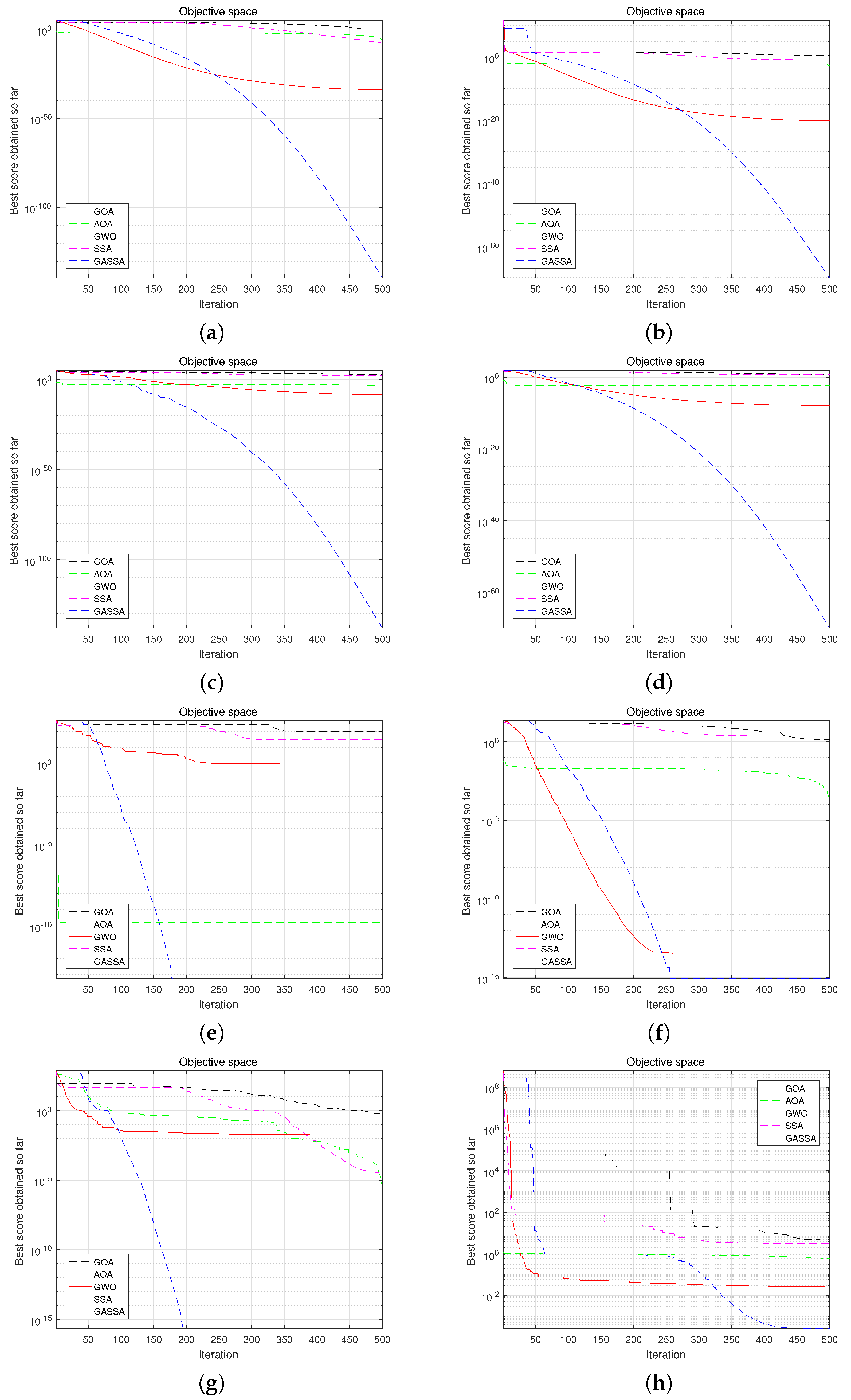
4.1. Evaluation of ISSA on Benchmark Functions

Benchmark function testing is a common method to measure the performance of intelligent algorithms. Eight benchmark test functions are selected to demonstrate the superior performance of the improved algorithms. $F_1$−$F_4$ are single-peak functions, and only one optimal solution exists for these types of test functions. This type of search space is suitable for testing the speed of convergence and the ability to search. $F_5$−$F_8$ are multi-peak benchmark functions. There exist local optima for multi-peak benchmark functions, which makes them suitable for comparing the local optimal avoidance and exploration behavior of the algorithm. Their specific information is shown in

Table 1. Benchmark test functions.

Funtion	Dim	Domain	Optimum Value
$F_1\left(x\right)={\sum }_{i=1}^n{x}_i^2$	30	[−100,100]	0
$F_2\left(x\right)={\displaystyle \sum _{i=1}^n}\left|x_i\right|+{\displaystyle \prod _{i=1}^n}\left|x_i\right|$	30	[−10,10]	0
$F_3\left(x\right)={\displaystyle \sum _{i=1}^n}\left({\displaystyle \sum _{j-1}^i}{x}_j\right)$	30	[−100,100]	0
$F_4\left(x\right)={max}_i\left\{\left|x_i\right|,1\le i\le n\right\}$	30	[−100,100]	0
$F_5\left(x\right)={\displaystyle \sum _{i=1}^n}\left[x_i^2-10\cos \left(2\pi x_i\right)+10\right]$	30	[−5.12,5.12]	0
$\begin{array}{c}\hfill F_6\left(x\right)=-20exp\left(-0.2\sqrt{\frac{1}{n}\sum _{i=1}^n{x}_i^2}\right)-exp\left(\frac{1}{n}\sum _{i=1}^{n}cos\left(2\pi x_i\right)\right)+20+e\end{array}$	30	[−32,32]	0
$F_7\left(x\right)=\frac{1}{4000}{\sum }_{i=1}^n{x}_i^2-{\prod }_{i=1}^{n}cos\left(\frac{x_i}{\sqrt{i}}\right)+1$	30	[−600,600]	0
$\begin{array}{c}{F}_8\left(x\right)=\frac{\pi }{n}\left\{10sin\left(\pi y_1\right)+{\displaystyle \sum _{i=1}^{n-1}}{\left(y_i-1\right)}^2\left[1+10{sin}^2\left(\pi y_{i+1}\right)\right]+{\left(y_n-1\right)}^2\right\}+{\displaystyle \sum _{i=1}^n}u\left(x_i,10,100,4\right)\\ y_i=1+\frac{x_i+1}{4}\\ u\left(x_i,a,k,m\right)=\left\{\begin{array}{c}k{\left(x_i-a\right)}^m{x}_i>a\\ 0-a<x_i<a\\ k{\left(-x_i-a\right)}^m{x}_i<-a\end{array}\right.\end{array}$	30	[−50,50]	0

.

To verify the effectiveness of GASSA, the performance of GASSA is compared with the standard salp swarm algorithm (SSA) and a series of well-known meta-heuristic algorithms, namely the standard gray wolf optimization algorithm (GWO) [33], the standard grasshopper optimization algorithm (GOA) [34] and the standard arithmetic optimization algorithm (AOA) [35]. In addition, the parameters of the comparison algorithm in the paper remain consistent with the original paper. For the fairness of the comparison, the parameters of all algorithms are set to be the same: population size is N = 60 and the number of iterations is $L_{max}$ = 500. The experimental environment of this paper is based on Intel®CoreTMi5-7200 CPU with 2.5 GHz main frequency and Windows 10 operating system with 4 GB of memory. To reduce the chance error of the experiment, each algorithm is run 30 times independently in each function. The results are taken as the best value, the worst value, the average value and the standard deviation, as shown in

Table 2. Results of benchmark test functions.

Funtion	Criteria	GOA	AOA	GWO	SSA	GASSA
$F_1$	Best Worst Mean Std	6.3653 0.3697 1.8666 1.306	2.61E-06 3.48E-08 1.33E-06 5.76E-07	1.81E-34 6.71E-37 3.01E-35 5.00E-35	2.28E-08 8.81E-09 1.62E-08 3.88E-09	6.95E-140 2.37E-140 4.81E-140 1.28E-140
$F_2$	Best Worst Mean Std	7.8752 0.5053 2.9865 1.6878	0.0037 9.29E-13 4.54E-04 8.75E-04	8.05E-21 8.01E-22 4.02E-21 1.94E-21	2.7071 0.0024 0.6907 0.7423	1.14E-70 7.40E-71 9.17E-71 1.10E-71
$F_3$	Best Worst Mean Std	2.22E+03 477.663 1.08E+03 579.2324	0.0015 1.42E-05 3.47E-04 3.15E-04	7.26E-09 3.56E-12 9.72E-10 1.63E-09	874.2436 75.0897 339.2362 210.5062	1.73E-138 7.45E-140 7.73E-139 5.77E-139
$F_4$	Best Worst Mean Std	12.7393 3.8623 7.8885 2.6074	0.0355 5.31E-04 0.0092 0.0086	3.52E-08 5.03E-10 7.49E-09 8.37E-09	10.2434 0.9004 5.4139 2.7326	1.24E-70 7.44E-71 9.38E-71 1.20E-71
$F_5$	Best Worst Mean Std	108.56 36.8248 65.2024 22.2072	1.26E-06 0 3.95E-07 4.48E-07	7.867 0 1.6685 2.7474	71.6369 17.9093 40.6606 13.4296	0 0 0 0
$F_6$	Best Worst Mean Std	4.3593 1.9727 2.968 0.7744	4.05E-04 3.63E-06 2.39E-04 1.04E-04	5.06E-14 2.93E-14 3.78E-14 4.72E-15	3.28E+00 3.48E-05 1.8597 0.6383	8.88E-16 8.88E-16 8.88E-16 0
$F_7$	Best Worst Mean Std	0.7141 0.2833 0.5249 0.1303	0.0197 3.45E-06 6.64E-04 0.0036	0.0338 0 0.0071 0.0102	0.032 1.92E-06 0.0103 0.0099	0 0 0 0
$F_8$	Best Worst Mean Std	11.5914 2.7514 5.8342 2.9491	0.6629 0.5459 0.6058 0.0289	0.0458 0.0058 0.0196 0.0109	10.1161 1.2637 4.6115 1.8673	0.0252 1.2706e-05 0.0042 0.0071

.

Table 3. Average computation time (in seconds) of 5 algorithms on 8 benchmark functions.

Function	GOA	AOA	GWO	SSA	GASSA
$F_1$	269.278	0.7114	1.0598	0.6286	0.7394
$F_2$	250.785	0.7466	1.0821	0.6239	0.7458
$F_3$	261.153	2.1571	2.4746	2.0541	2.2215
$F_4$	243.992	0.8495	1.1084	0.6534	0.7567
$F_5$	212.327	0.7871	1.1723	0.6936	1.5918
$F_6$	235.341	0.8496	1.2113	0.7198	1.6647
$F_7$	240.101	0.9282	1.3054	0.8385	1.8246
$F_8$	259.278	1.4948	1.8724	1.3668	3.1296

shows the average computation time for the five algorithms on the eight benchmark functions. The best results for each function are highlighted in bold.

As can be seen from Table 2, GASSA achieves better results in the test results of single-peak benchmark test functions $F_1$−$F_4$. All indexes of GASSA have significant advantages compared with other algorithms. The mean value can reflect the convergence of the algorithm, which shows that GASSA has better convergence and higher convergence accuracy than other compared algorithms. It shows that the proposed improvement strategy can effectively improve the convergence accuracy of SSA. The standard deviation can reflect the dispersion degree of the data set. The smaller the standard deviation indicates that the dispersion degree of the data set is lower and the stability of the experimental results is better.

In the test results of multi-peak benchmark functions $F_5$−$F_8$, GASSA outperforms the standard SSA and other algorithms in the mean and standard deviation of the optimal solution, which indicates that the improved algorithm has good ability to avoid falling into local optimum. However, the accuracy of the solution on some multi-peak functions is lower than that of single-peak functions, which indicates that the algorithm is inadequate for solving multi-peak functions. This is a direction for further research. The computational cost in Table 3 shows that SSA has the lowest time cost, and GASSA has the moderate time cost; however, GOA has the considerable time cost for all benchmark functions.

The performance of an algorithm can be shown visually by the convergence curve, which shows the number of times the algorithm falls into the local optimum and the speed of convergence. Since the multi-peaked functions are more complex and easy to make the algorithm fall into local extremes, the convergence curve of these functions is more indicative of the algorithm’s ability to find the best. Therefore, Figure 5 shows the convergence curves of GWO, AOA, GOA, SSA, and GASSA on eight functions.

The convergence curves of the eight functions clearly show the trend of the fitness values of the five algorithms in the evolutionary process. As shown in Figure 5a,b,f, AOA, GOA, and SSA converge slowly, while GWO converges fast in the early iterations. However, GWO quickly falls into local optima that cannot be jumped out, and the convergence accuracy of GWO, AOA, GOA and SSA at the end of the iteration is lower than that of GASSA. In Figure 5c,d,g, GASSA has faster convergence speed and accuracy than the other four algorithms. In Figure 5e,h, AOA, GWO, SSA and GOA all have the problem of fast convergence in the early stage but easily fall into local optimum, and the convergence accuracy is lower than that of GASSA. From the above analysis, it can be seen that GASSA has significantly better optimization-seeking accuracy and convergence performance than the other four algorithms.

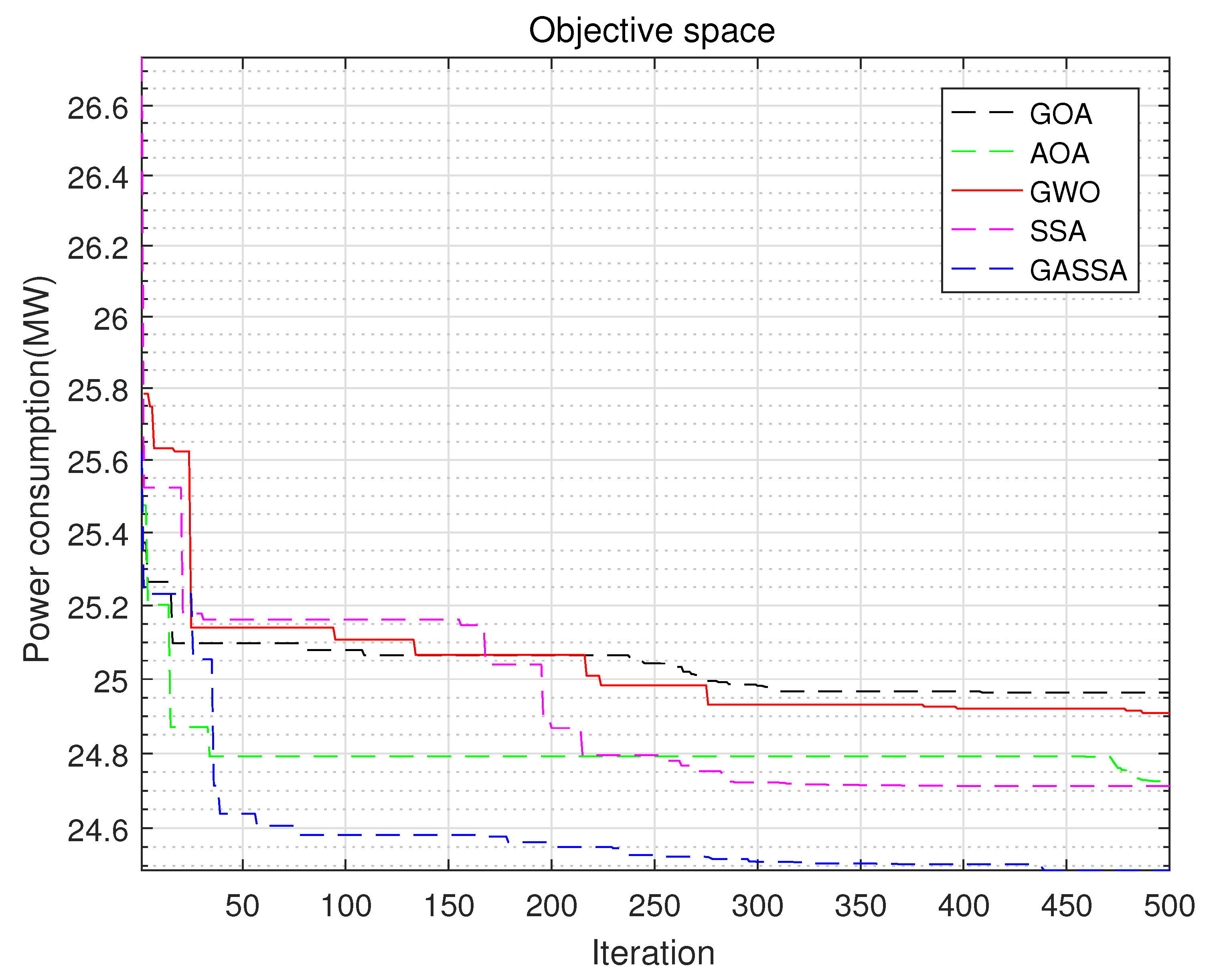
4.2. Evaluation of ISSA on Load-Sharing Optimization

In this section, we consider the GASSA application for a booster compressor station consisting of six parallel compressors.

Table 4. The main parameters of the simulated operation of the booster compressor station.

Parameters	Value
Suction pressure ($\mathrm{MPa}$)	3.3
Suction temperature ($\mathrm{K}$)	293.15
Gas constant ($\mathrm{J}/\mathrm{kg}·\mathrm{K}$)	518.75
Total volume flow rate (${\mathrm{m}}^3/\mathrm{s}$)	15
Compressor ratio	1.5

shows the main parameters of the booster compressor station operation in this case. The six compressors can be classified into four types: one type A (Compressor No. 1), three type B (Compressor No. 2 to 4), one type C (Compressor No. 5) and one type D (Compressor No. 6).

Table 5. Parameters of the four types of compressors.

Parameter	A-Type	B-Type	C-Type	D-Type
$a_1$	0.835	0.918	0.572	0.547
$a_2$	1.01E-05	1.30E-05	6.9E-06	2.62E-05
$a_3$	6.29E-08	3.87E-08	9.93E-08	5.18E-08
$a_4$	0.226	0.226	0.834	−0.0177
$a_5$	0.000644	0.000644	0.000417	0.00099
$a_6$	5.09E08	5.09E-08	1.00E-07	2.56E-08
$b_1$	0.00215	0.00198	0.0034	0.001923
$b_2$	0.515	0.515	0.488	2.72
$b_3$	−1564	−1564	−1481	−2174
$b_4$	0.607	0.636	0.528	0.405
$b_5$	877	751	921	1252
$b_6$	−700,000	−614,000	−650,000	−844,000
$N_{min}$	3965	3965	3120	3380
$N_{max}$	6405	6405	5040	5460

provides the parameters of the model compressor under this operating condition, which can be used to calculate the parameters of the compressor working domain.

To further demonstrate the superiority of GASSA, it is compared with the standard SSA, GWO, GOA and AOA. The parameters of each algorithm are set as follows: the population size is N = 50 and the maximum number of iterations is $L_{max}$ = 500. In addition, all algorithms are run 30 times independently, and the results are taken as the best value, the worst value, the average value and the standard deviation, as shown in

Table 6. Statistics of the results of 30 calculations.

Power Consumption (MW)	GOA	AOA	GWO	SSA	GASSA
Best	24.5371	24.5132	24.5192	24.5069	24.4878
Worst	25.1881	25.1184	25.1748	25.0106	24.782
Mean	24.8105	24.8043	24.7988	24.6998	24.6022
Std	0.1822	0.1561	0.1446	0.1322	0.0668

.

Table 7. Optimal load-sharing scheme.

Algorithm	NO.1	NO.2	NO.3	NO.4	NO.5	NO.6
GOA	3.6630	3.4148	3.7158	4.2065	0	0
AOA	3.9099	3.8071	3.7392	3.5437	0	0
GWO	3.7975	3.3440	4.0933	0	0	3.7652
SSA	3.5098	0	4.0020	3.9907	0	3.4975
GASSA	3.8135	3.7715	3.8502	0	0	3.5647

shows the optimal solutions corresponding to the optimal values.

Table 8. Average computation time (in seconds) of 5 algorithms on the simulation case.

Computation Time	GOA	AOA	GWO	SSA	GASSA
Average value	43.6421	0.6173	0.5883	0.6038	0.6209

shows the average computation time of the five algorithms in the case. The best results for each algorithm are highlighted in bold. Figure 6 shows the convergence graph of GASSA in solving the model.

According to the optimized results of the five algorithms in Table 6 and Table 7, we can find that the GASSA optimization results in significant power savings compared to other algorithms, which indicates that GASSA has the potential to reduce the operating cost of the booster compressor station. Specifically, among the four standard algorithms, SSA obtains the minimum power consumption for the minimum value, maximum value, and average value, and the standard deviation is the best. However, GASSA provides better metrics compared with SSA. For example, the optimal and average power consumption of GASSA is 0.0191 $\mathrm{MW}$ and 0.0976 $\mathrm{MW}$ higher than SSA, respectively. This indicates that the optimization results of GASSA are not only high in accuracy, but also the stability of the solution is significantly better than other algorithms. Although AOA and GWO take less time on average than GASSA, AOA has lower convergence accuracy. In Figure 6, the GWO converges very slowly and stalls in the iterative process, which is very easy to fall into local optimum. Overall, GASSA shows the high competitive ability in finding the global optimal solution within a reasonable time consumption.

Regarding the convergence curves in Figure 6, the convergence curves of the five algorithms keep falling in the initial iterations as the number of iterations increases. The convergence of SSA is slower compared to GASSA due to the random initialization of populations, which leads to the non-uniform distribution of population distributions in space. At this time, the convergence of GASSA is slower compared to AOA because the higher percentage of leaders in GASSA focuses more on global search rather than local exploration. However, as the number of followers increases and the random inertia weights come into play, GASSA has the stronger ability to get rid of the local optimum. Later in the iteration, other algorithms have fallen into local optima and the curve stalls, while the convergence curve of GASSA still continues to fall and converge to the better result.

5. Conclusions

In this paper, we propose an accurate and reliable algorithm to solve the nonlinearity and nonconvex MINLP model for optimization of load distribution of the booster compressor station to reduce the operating cost of the booster compressor station. Specifically, instead of using binary variables to indicate the on or off state of the compressor, semi-continuous variables are utilized to describe the flow variation and on or off state of the compressor. Thus, the number of variables is reduced and the search space is simplified. In addition, a new salp swarm algorithm (GASSA) is proposed to solve this model. In GASSA, the good point set strategy is used to initiate the population in order to increase the variety of the population; to improve the global search and local exploitation capability of the algorithm, the adaptive population division constantly modifies the population’s leader-to-follower ratio; adaptive inertia weights are added to the mechanism of the followers to help the followers jump out of the local optimum.

Comprehensive experiments are conducted on eight benchmark test functions and one simulation case to verify the performance of GASSA. The test results of the benchmark functions show that GASSA is stronger than other algorithms in terms of optimization accuracy and reliability. The case results show that GASSA improves the optimal power consumption and average power consumption by 0.0191 $\mathrm{MW}$ and 0.0976 $\mathrm{MW}$, respectively, compared to the best-performing algorithm among the others. Therefore, GASSA is a promising candidate for optimizing the load distribution in the booster compressor station.

References

1. Lu, S.; Fang, M.; Wang, Q.; Huang, L.; Sun, W.; Zhang, Y.; Li, Q.; Zhang, X. Public Acceptance Investigation for 2 Million Tons/Year Flue Gas CO2 Capture, Transportation and Oil Displacement Storage Project. Int. J. Greenh. Gas Control. 2021, 111, 103442. [Google Scholar] [CrossRef]
2. Arya, A.K.; Honwad, S. Modeling, Simulation, and Optimization of a High-Pressure Cross-Country Natural Gas Pipeline: Application of an Ant Colony Optimization Technique. J. Pipeline Syst. Eng. Pract. 2016, 7, 04015008. [Google Scholar] [CrossRef]
3. Wang, B.; Liang, Y.; Yuan, M. Water Transport System Optimisation in Oilfields: Environmental and Economic Benefits. J. Clean. Prod. 2019, 237, 117768. [Google Scholar] [CrossRef]
4. Sadeghi, Z.; Horry, H.R.; Khazaee, S. An Economic Evaluation of Iranian Natural Gas Export to Europe through Proposed Pipelines. Energy Strategy Rev. 2017, 18, 1–17. [Google Scholar] [CrossRef]
5. Vahdati, N.; Wang, X.; Shiryayev, O.; Rostron, P.; Yap, F.F. External Corrosion Detection of Oil Pipelines Using Fiber Optics. Sensors 2020, 20, 684. [Google Scholar] [CrossRef] [Green Version]
6. Lu, H.; Ma, X.; Azimi, M. US Natural Gas Consumption Prediction Using an Improved Kernel-Based Nonlinear Extension of the Arps Decline Model. Energy 2020, 194, 116905. [Google Scholar] [CrossRef]
7. Bagheri, M.; Sari, A. Study of Natural Gas Emission from a Hole on Underground Pipelines Using Optimal Design-Based CFD Simulations: Developing Comprehensive Soil Classified Leakage Models. J. Nat. Gas Sci. Eng. 2022, 102, 104583. [Google Scholar] [CrossRef]
8. Su, Z.; Liu, E.; Xu, Y.; Xie, P.; Shang, C.; Zhu, Q. Flow Field and Noise Characteristics of Manifold in Natural Gas Transportation Station. Oil Gas Sci. Technol.—Revue d’IFP Energies Nouv. 2019, 74, 70. [Google Scholar]
9. Liu, K.; Biegler, L.T.; Zhang, B.; Chen, Q. Dynamic Optimization of Natural Gas Pipeline Networks with Demand and Composition Uncertainty. Chem. Eng. Sci. 2020, 215, 115449. [Google Scholar] [CrossRef]
10. Liu, E.; Lv, L.; Ma, Q.; Kuang, J.; Zhang, L. Steady-State Optimization Operation of the West–East Gas Pipeline. Adv. Mech. Eng. 2019, 11, 1687814018821746. [Google Scholar] [CrossRef] [Green Version]
11. Kumar, S.; Cortinovis, A. Load Sharing Optimization for Parallel and Serial Compressor Stations. In Proceedings of the 2017 IEEE Conference on Control Technology and Applications (CCTA), Maui, HI, USA, 27–30 August 2017; pp. 499–504. [Google Scholar]
12. Deng, T. Minimization of Power Usage in a Compressor Station with Multiple Compressors. J. Energy Eng. 2016, 142, 04015048. [Google Scholar] [CrossRef]
13. Wu, S.; Ríos-Mercado, R.Z.; Boyd, E.A.; Scott, L.R. Model Relaxations for the Fuel Cost Minimization of Steady-State Gas Pipeline Networks. Math. Comput. Model. 2000, 31, 197–220. [Google Scholar] [CrossRef]
14. Milosavljevic, P.; Marchetti, A.G.; Cortinovis, A.; Faulwasser, T.; Mercangöz, M.; Bonvin, D. Real-Time Optimization of Load Sharing for Gas Compressors in the Presence of Uncertainty. Appl. Energy 2020, 272, 114883. [Google Scholar] [CrossRef]
15. Cortinovis, A.; Mercangöz, M.; Zovadelli, M.; Pareschi, D.; De Marco, A.; Bittanti, S. Online Performance Tracking and Load Sharing Optimization for Parallel Operation of Gas Compressors. Comput. Chem. Eng. 2016, 88, 145–156. [Google Scholar] [CrossRef]
16. Zapukhliak, V.; Poberezhny, L.; Maruschak, P.; Grudz, V., Jr.; Stasiuk, R.; Brezinová, J.; Guzanová, A. Mathematical Modeling of Unsteady Gas Transmission System Operating Conditions under Insufficient Loading. Energies 2019, 12, 1325. [Google Scholar] [CrossRef] [Green Version]
17. Liu, E.; Lv, L.; Yi, Y.; Xie, P. Research on the Steady Operation Optimization Model of Natural Gas Pipeline Considering the Combined Operation of Air Coolers and Compressors. IEEE Access 2019, 7, 83251–83265. [Google Scholar] [CrossRef]
18. Rodrigues, L.R. A Hybrid Multi-Population Metaheuristic Applied to Load-Sharing Optimization of Gas Compressor Stations. Computers Electr. Eng. 2022, 97, 107632. [Google Scholar] [CrossRef]
19. Li, X.; Cui, T.; Huang, K.; Ma, X. Optimization of Load Sharing for Parallel Compressors Using a Novel Hybrid Intelligent Algorithm. Energy Sci. Eng. 2021, 9, 330–342. [Google Scholar] [CrossRef]
20. Mirjalili, S.; Gandomi, A.H.; Mirjalili, S.Z.; Saremi, S.; Faris, H.; Mirjalili, S.M. Salp Swarm Algorithm: A Bio-Inspired Optimizer for Engineering Design Problems. Adv. Eng. Softw. 2017, 114, 163–191. [Google Scholar] [CrossRef]
21. Pavan Kumar Neeli, V.S.R.; Salma, U. Automatic Generation Control for Autonomous Hybrid Power System Using Single and Multi-objective Salp Swarm Algorithm. In Proceedings of the Intelligent Computing, Information and Control Systems, Madurai, India, 15–17 May 2019; Springer: Cham, Switzerland, 2020; pp. 624–636. [Google Scholar]
22. Yang, B.; Zhong, L.; Zhang, X.; Shu, H.; Yu, T.; Li, H.; Jiang, L.; Sun, L. Novel Bio-Inspired Memetic Salp Swarm Algorithm and Application to MPPT for PV Systems Considering Partial Shading Condition. J. Clean. Prod. 2019, 215, 1203–1222. [Google Scholar] [CrossRef]
23. Zhang, J.; Wang, Z.; Luo, X. Parameter Estimation for Soil Water Retention Curve Using the Salp Swarm Algorithm. Water 2018, 10, 815. [Google Scholar] [CrossRef] [Green Version]
24. Mahmoudimehr, J.; Sanaye, S. Minimization of Fuel Consumption of Natural Gas Compressor Stations with Similar and Dissimilar Turbo-Compressor Units. J. Energy Eng. 2014, 140, 04013001. [Google Scholar] [CrossRef] [Green Version]
25. Liu, E.; Li, C.; Yang, Y. Optimal Energy Consumption Analysis of Natural Gas Pipeline. Sci. World J. 2014, 2014, e506138. [Google Scholar] [CrossRef] [PubMed]
26. Borraz-Sánchez, C.; Haugland, D. Minimizing Fuel Cost in Gas Transmission Networks by Dynamic Programming and Adaptive Discretization. Comput. Ind. Eng. 2011, 61, 364–372. [Google Scholar] [CrossRef]
27. Paparella, F.; Domínguez, L.; Cortinovis, A.; Mercangöz, M.; Pareschi, D.; Bittanti, S. Load Sharing Optimization of Parallel Compressors. In Proceedings of the 2013 European Control Conference (ECC), Zurich, Switzerland, 17–19 July 2013; pp. 4059–4064. [Google Scholar]
28. Borraz-Sánchez, C.; Ríos-Mercado, R.Z. Improving the Operation of Pipeline Systems on Cyclic Structures by Tabu Search. Comput. Chem. Eng. 2009, 33, 58–64. [Google Scholar] [CrossRef]
29. Chen, Q.; Shen, Z.; Chen, Z. A Penalty Function Semi-Continuous Thresholding Methods for Constraints of Hashing Problems. J. Vis. Commun. Image Represent. 2022, 87, 103552. [Google Scholar] [CrossRef]
30. Toragay, O.; Silva, D.F.; Vinel, A.; Shamsaei, N. Exact Global Optimization of Frame Structures for Additive Manufacturing. Struct. Multidiscip. Optim. 2022, 65, 97. [Google Scholar] [CrossRef]
31. Ni, S.; Chen, W.; Ju, H.; Chen, T. Coordinated Trajectory Planning of a Dual-Arm Space Robot with Multiple Avoidance Constraints. Acta Astronaut. 2022, 195, 379–391. [Google Scholar] [CrossRef]
32. Arora, S.; Singh, S. Butterfly Optimization Algorithm: A Novel Approach for Global Optimization. Soft Comput. 2019, 23, 715–734. [Google Scholar] [CrossRef]
33. Mirjalili, S.; Mirjalili, S.M.; Lewis, A. Grey Wolf Optimizer. Adv. Eng. Softw. 2014, 69, 46–61. [Google Scholar] [CrossRef] [Green Version]
34. Saremi, S.; Mirjalili, S.; Lewis, A. Grasshopper Optimisation Algorithm: Theory and Application. Adv. Eng. Softw. 2017, 105, 30–47. [Google Scholar] [CrossRef] [Green Version]
35. Abualigah, L.; Diabat, A.; Mirjalili, S.; Abd Elaziz, M.; Gandomi, A.H. The Arithmetic Optimization Algorithm. Comput. Methods Appl. Mech. Eng. 2021, 376, 113609. [Google Scholar] [CrossRef]
Figure 1. Natural gas compressor station with parallel topology.
Energies 15 05720 g001
Figure 2. Compressor’s working domain.
Energies 15 05720 g002
Figure 3. Difference between binary and semi-continuous variables.
Energies 15 05720 g003
Figure 4. The flow chart of the proposed GASSA.
Energies 15 05720 g004
Figure 5. Convergence curve of benchmark functions. (a)  F 1 ; (b) F 2 ; (c) F 3 ; (d) F 4 ; (e) F 5 ; (f) F 6 ; (g) F 7 ; (h) F 8 .
Energies 15 05720 g005
Figure 6. Comparison of 5 algorithms for optimizing curve.
Energies 15 05720 g006