Air-Side Nusselt Numbers and Friction Factor’s Individual Correlations of Finned Heat Exchangers

Abstract

Currently, when designing finned heat exchangers (FHE), the average value of the entire heat transfer coefficient (HTC) is considered. However, each row of the heat exchanger (HEX) has different hydraulic-thermal characteristics. The novelty of this research is to present the differentiation of the individual air-side Nusselt number and Darcy-Weisbach friction factor correlations in each row of FHE using CFD modelling. FHE has four-rows, circular tubes, and continuous fins with a staggered tube arrangement. Relationships for the Nusselt number and D-W friction factor derived for the entire exchanger based on CFD modelling were compared with those available in the literature, determined using experimental data. The maximum relative differences between the Nusselt number for a four-row FHE determined experimentally and by CFD modelling are in the range from 22% for a Reynolds number based on a tube outside diameter of 1000 to 30% for a Reynolds number of 13,000. The maximum relative differences between the D-W friction factor for a four-row FHE determined experimentally and by CFD modelling are in the range of 50% for a Reynolds number based on a tube outer diameter of 1000 to 10% for a Reynolds number of 13,000. The CFD modelling performed shows that in the range of Reynolds numbers based on hydraulic diameters from 150 to 1400, the Nusselt number for the first row in a four-row FHE is about 22% to 15% higher than the average Nusselt number for the entire exchanger. In the range of Reynolds number changes based on hydraulic diameter from 2800 to 6000, the Nusselt numbers on the first and second rows of tubes are close to each other. Correlations of Nusselt numbers and D-W friction factors derived for individual tube rows can be used in the design of plate-fin and tube heat exchangers used in equipment such as air-source heat pumps, automotive radiators, air-conditioning systems, and in air hot-liquid coolers. In particular, the correlations can be used to select the optimum number of tube rows in the exchanger.

1. Introduction

Finned heat exchangers (FHE) are widely used in applications for renewable energy sources or zero-emission processes such as air heat pumps or exchangers for waste energy recovery [1]. The market for that equipment is growing significantly and will be and there is continued potential for growth due to the zero-emission policy, decarbonization, degasification, and geopolitical issues [2,3]. There is more and more research that discusses also increasing the heat transfer rate to limit the construction materials of any type of heat exchanger [4].

The problem of designing efficient finned air-heated heat exchangers is becoming increasingly important with the rapid development of air-source heat pumps. An experimental study of the hybrid indoor air conditioning system with an earth-to-air heat exchanger and air source heat pump is presented in [5]. The performance of the system was confirmed in the hot-summer and cold-winter regions of China. The improved performance of an air heat pump heating system with variable water temperature differences is demonstrated in [6]. A large water temperature difference for the air heat pump heating system was first proposed.

FHEs have also been widely used in recent years in PCM (Phase Change Materials) heat accumulators [7]. Due to the slow heating and cooling of the heat storage fill, a phase change occurs only near the heat exchanger tubes [8]. Much of the material stored in the PCM accumulator is dead and does not undergo a phase change. The use of a heat exchanger with finned tubes accelerates the melting and heating of PCM throughout the entire volume of the accumulator [8]. Fin arrays of non-uniform dimensions and different distribution patterns were investigated to determine the impact of modified fin design on the performance of latent heat storage units [9]. The foam strip-fin combination for enhancing the thermal response of the PCM storage unit was studied in [10]. Faster melting and solidification rates, up to 58 and 42% respectively, were achieved compared to the full foam. A vertical counter-flow triple tube heat exchanger was used to heat or to cool the PCM [11]. Circular fins with staggered distribution were applied to attain improved thermal response rates of the PCM heat storage unit.

The minimizing equipment has a positive effect on reducing the noise generated by the unit and the total pressure drop on the gas side [1]. So, is it also possible to minimize finned heat exchanger [12]? Can local values of air-side heat transfer coefficient (HTC) be applied to air heat pump? Can you do the same for all finned heat exchangers [13]?

Even though, science does not have a full understanding of FHE with its complicated phenomena on the air- and water-side [14]. Individual rows function differently. It depends on the FHE geometry and more newly developed geometries are described. Bošnjaković and Muhič [15] presented star fin shape of FHE. Variability is due to the different air and water temperatures and airflow vortexes and velocity.

Despite the rapid development of CFD modelling of flow and thermal processes occurring in heat exchangers, engineering calculation methods based on analytical formulas are also being developed [16].

Still, there is a lot of research for experimentally or numerically determining the average HTC of FHE. Those HTCs are used in the standard designing process of FHE [14]. Sadeghianjahromi and Wang [17] collected several dozen average HTC of FHE for different fin geometries: plain, louvre, wavy, and plain with vortex generation. This research presented a detailed review of experimental considers heat transfer and pressure drop characteristics of enhancements. Zhang et al. [18] presented experimentally determine characteristics of airfoil fin heat exchanger. The research showed that the pressure drop in the airfoil fin heat exchanger is only about 1/6 of that in the zigzag channel FHE with a comparative heat transfer rate. Average HTCs are also widely used during evaporation or condensation heat transfer. Jige et al. [19] researched the two-phase evaporation flow of FHE using thermodynamic fluids: R32 and R1234ze(E). The authors noticed that in some region of the FHE, the HTC are significantly smaller than in the rest of the FHE regions, due to the formed dry area, which decrease HTC. Vaisi et al. [20] presented heat transfer characteristics during condensation flow in FHE with two types of fins. The authors spotted also, that higher wave amplitude to wavelength ratios, lower pitch to height ratio of the fins, lower wavelength to fin length ratios, and lower fin pitch to wave amplitude ratios are obtained a higher thermal performance factor. Xie et al. [21] presented average heat transfer correlations of FHE. They have been designated numerically, although for the large tube diameter from 16 mm to 20 mm. This research showed that HTC dropped as the tube diameter increasd. Kim et al. [22] experimentally researched Colburn factors of FTE for large fin pitch from 7.5 mm to 15 mm. It turned out that j-factor is higher for fin pitch 15 mm than for fin pitch 7.5 mm and surprisingly this experiment showed that the average j-factor for four-row FHE is higher than for eight-row FHE.

Studies are appearing that involve local HTC of FHE. These studies usually describe the local heat exchange and often compare it to the average HTC. Che and Elbel [23] showed the experimental and numerical determination of heat transfer coefficients (HTCs) using the absorption-based mass transfer method. This study showed that the HTC value in the first row of FHE compared to the second row of FHE can be 30% higher. Węglarz et al. [24] presented a new analytical method for the thermal calculation of FHE. This method can use individual or average correlation of HTC, Nusselt number or Colburn factor. Marcinkowski et al. [25] compared individual rows of tube air-side Nusselt numbers to average HTC in the entire FHE. This investigation showed that the heat flow rate transferred in the first rows of tubes can reach up to 65% of the heat output of the entire exchanger.

The geometry of the modeled FHE was selected from the Kelvion manufacturer’s website (

Table 1. Dimensions of the modelled FHE [26].

Description	Designation	Value
Rows	-	4
Transversal tube pitch	$p_t$	32 mm
Longitudinal tube pitch	$p_l$	27.71 mm
Tube outer diameter	$d_o$	12 mm
Fin pitch	$s$	3 mm
Fin thickness	${\delta }_f$	0.14 mm
Fin length of single row	$L_r$	27.71 mm

) [26]. Similar geometries and air speed ranges were also analysed by two other research teams. The results of this paper were compared to the existing experimental results to verify the accuracy of calculations. In the first study, Wang et al. [27] compared correlations for dry and wet conditions. The authors concluded that the sensible j factors under dehumidifying conditions are not dependent on inlet air parameters. Furthermore, they showed that in the case of a completely wet surface, the f factors do not change as a function of the inlet air parameters and, moreover, change slightly as a function of the fin pitch and the number of tube rows. In the second study, Wang et al. [28] presented a semi universal correlation which considers not only Reynolds number, but also the fin pitch, fin thickness, the outer tube diameter and the number of tube rows.

Although the above-mentioned researches have been studied in detail, insufficient attention has been paid to local air flow behavior as Nusselt number and Darcy Weisbach friction factor correlations [13]. This paper presents not only the correlations but also a simple, easily repetitive method to determine those correlations. The novelty of the current study is to numerically investigate individual HTC and individual pressure drops through Nusselt number and Darcy-Weisbach (D-W) friction factor on each row of tubes of FHE. In the end, by virtue of, using a commonly available geometry from one of the exchanger manufacturers [23], the results of this paper could have greater utility.

The experimental result [13,29] shows that there are significant differences of coefficient between an individual row of tubes. This is true especially if air velocity in front of FHE is smaller than 2.5 m/s [13]. It is possible to consider different coefficients on each row of tubes. Considering these dependencies between heat transfer coefficient and the row’s position will allow optimal FHE design, e.g., it will eliminate four-row FHEs in favor of one- or two-row FHEs. Following optimization could give a chance to reduce materials for building FHEs.

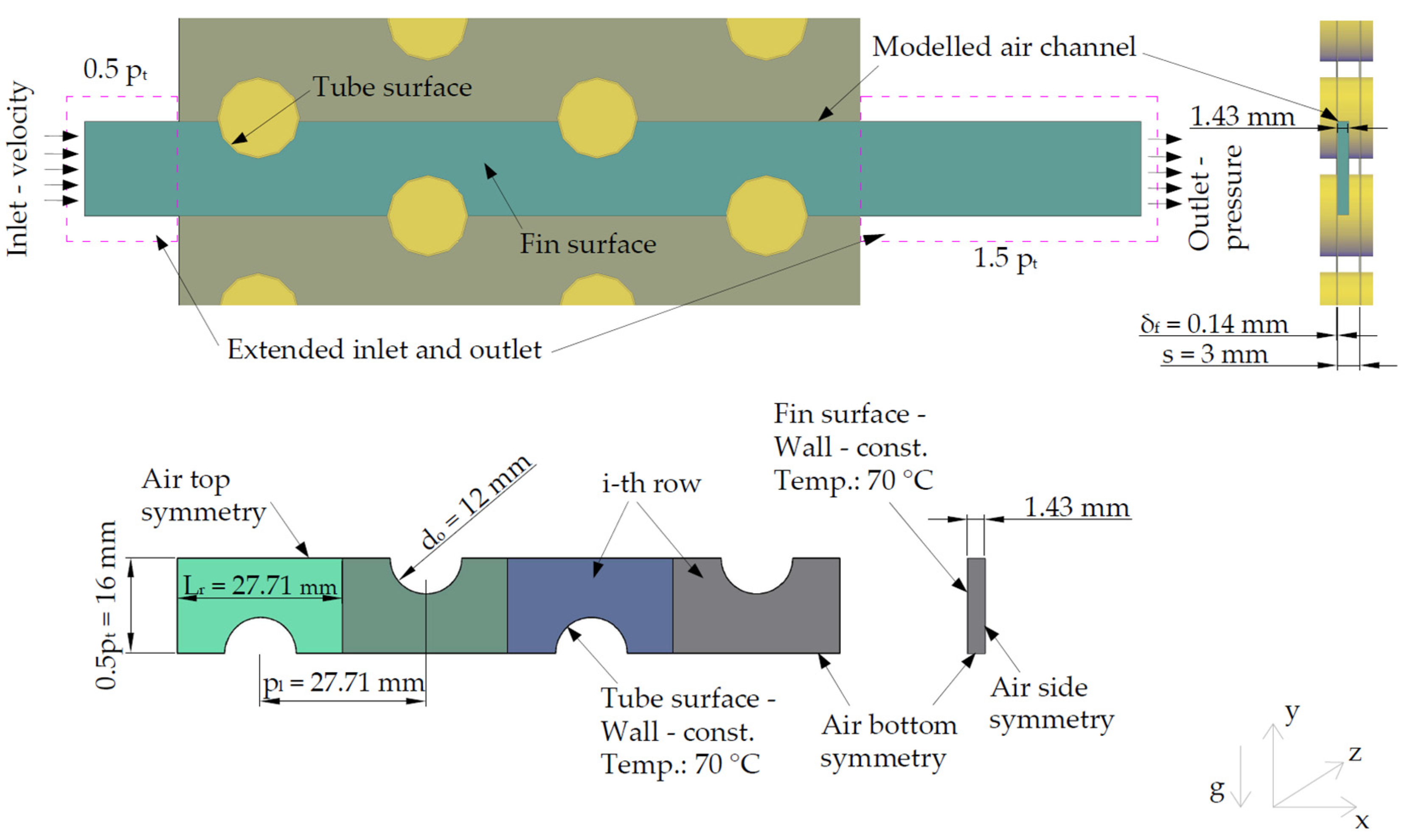
2. Geometry and CFD Model

Table 1 shows data set of the materials and dimensions of the modelled FHE. These dimensions are taken from FHE Kelvion producer webpage [26]. The fin pitch $s$ of FHE equals 3 mm. However, the width of the modelled air volume contains only half of them 1.5 mm and it is reduced by the thickness of half a fin 0.07 mm. Where fin thickness ${\delta }_f$ equals 0.14 mm. Thus the modelled width is 1.43 mm. The following simplifications are allowed due to the air symmetry from third directions: top, bottom, and side. The tube outer diameter $d_o$ equals 12 mm. The transversal tube pitch is 32 mm. However, the height of the modelled volume equals $0.5 p_t=16 \mathrm{mm}$, also due to the air symmetry. The longitudinal tube pitch is 27.71 mm, and the length of each row equals 27.71 mm (Figure 1).

Figure 1 presents a repetitive segment of the air between one fin pitch in analysed FHE. Figure 1 shows also an extended inlet and outlet zone, which is necessary for correct model for upstream and downstream pressure fields [29]. Multiple researches that show the results of CFD modelling also include extended inlet and outlet zones. However, relating them to the different parameters such as: tube outer dimension $d_o$ [29], fin spacing $s$ and longitudinal tube pitch $p_l$ [30], channel height ($0.5 p_t$) [31], length of the tube bank (flow length) [32,33]. This paper adopted the following values, the inlet zone equals $0.5 p_t$ = 16 mm and the outlet zone is $1.5 p_t$ = 48 mm. Where the tube bank of four rows equals 110.84 mm.

The boundary conditions of the Ansys Fluent software are shown in Figure 1. Air Inlet is set at a constant temperature: 20 °C. Air outlet is set as an opening condition with verification mass average temperature in the outlet cross section of the air. The modelled air zone have symmetry conditions from the top, bottom and side. Wall boundary conditions is set on the opposite surface (fin surface) from the air symmetry side. This boundary conditions is marked by constant temperature: 70 °C. The same conditions with the same constant temperature are set on the tube surfaces. The different constant temperature of the fin and tubes surface in range from 60 °C to 80 °C cause a slight discrepancies, less than 1.6% compare to the constant temperature in current study: 70 °C [25]. The proposed conditions are universal and they can be used in water to air finned heat exchange where we have changing fluid and gas temperature, and also in evaporator or condenser, where we have constant temperature of phase transition and on the other side changing temperature of fluid or gas, what is most commonly used in air heat pumps or air conditioning.

Figure 2 presents finite element mesh of the repetitive fragment of the modelled FHE. The mesh has been divided into couple of volumes for better arrangement into equal parts. Particular colours in the Figure 2 present this division. Additionally, the compaction of the mesh has done at the fin and tubes surfaces. The compaction is shown in zoom windows in Figure 2. The regularity of the volumes are disturbed in the compaction zone, because elements are extended and inclined. However, deformation of the volumes is within acceptable limits. The minimum orthogonal angle is 35.6°. The mesh expansion factor equals 14 and the maximum aspect ratio is 22.

3. Assumptions and Data Reduction

This research shows a steady-state and three-dimensional (3D) computational fluid dynamics (CFD) simulation. The main assumptions are:

• Fixed inlet air temperature: 20 °C.
• Air outlet opening condition-control of medium mass air temperature in the outlet section.
• Fixed air-side fins and tubes surface temperature: 70 °C.
• Air parameters variable as a function of temperature.
• Reynolds-Averaged Navier-Stokes equations of the mass, momentum, and energy conservation were used
• Shear Stress Transport turbulence model.
• The residuals were set to less than The residuals were set to less than 10⁻³ for the continuity equations and 10⁻⁵ for the energy equations, respectively, to ensure that the calculations converge.
• The simulations were done by ANSYS-CFX 2020 R2 software.

The governing equations, i.e., conservation equations of mass, momentum, and energy given in [34] were used to model flow and heat transfer on the air side. The mathematical model is based on the hydraulic diameter $d_h$, which is calculated using the definition proposed by Kays and London [35] and maximum air velocity $w_{max}$ [35] in the minimum cross-section area $A_{min}$. The hydraulic diameter (Equation (1)) has been calculated by assumption dividing the volume through which air flows in one row (Equation (2)) by the surface area in contact with the air (Equation (3)).

$$d_h=\frac{4V_o}{A}$$

(1)

$$V_o=V_a-V_t$$

(2)

$$A=A_f+A_t$$

(3)

The symbol $V_o$ designates the volume through which air flows in one row. The symbol $A$ denotes total area in one row. Other symbols represent: $V_a$ the total volume of one row, $V_t$ the volume of tube in one row, $A_f$ the fin area in one fin pitch, $A_t$ the bare tube area in one row between two next fins.

$$V_a=p_l{p}_t\left(s-{\delta }_f\right)$$

(4)

$$V_t=\pi {\left(\frac{d_o}{2}\right)}^2\left(s-{\delta }_f\right)$$

(5)

$$A_f=2(p_l{p}_t-{\left(\pi \frac{d_o}{2}\right)}^2)$$

(6)

$$A_t=\pi d_o\left(s-{\delta }_f\right)$$

(7)

The symbol $p_l$ denotes the longitudinal fin pitch, the symbol $p_t$ designates the transverse fin pitch. Ither symbol represent: $s$ the fin pitch, ${\delta }_f$ the fin thickness, $d_o$ the outer tube diameter.

Equation (8) shows the full form of Equation (1) including Equations (4)–(7). The most often, the hydraulic diameter in the case of FHE is a slightly smaller than double fin pitch, and using geometry from Figure 1, equals 5.35 mm.

$$d_h=\frac{4\left(s-{\delta }_f\right)\left(p_l{p}_t-\pi {\left(\frac{d_o}{2}\right)}^2\right)}{2\left(p_l{p}_t-{\left(\pi \frac{d_o}{2}\right)}^2\right)+\pi d_o\left(s-{\delta }_f\right)}$$

(8)

The symbol $w_{\mathit{max}}$ is given by Equation (9). Parameter $w_{\mathit{max}}$ has been calculated for the minimum airflow cross-section between tubes [35] and it can exist in a different place in case of different FHE construction (Figure 1).

$$w_{\mathit{max}}=\frac{\left(s\cdot p_l\right)}{\left(s-{\delta }_f\right)\cdot \left(p_l-d_{o,min}\right)}\cdot \frac{\left({\overline{T}}_a^i\right)}{\left({\overline{T}}_{a,o}\right)}\cdot w_o$$

(9)

The symbol $w_{\mathit{max}}$ denotes the air velocity in the minimum cross-section of the air flow. The symbol $d_{o,min}$ the minimum dimension between tubes, ${\overline{T}}_a^i$ the mass average air temperature in i-th row of FTHE, ${\overline{T}}_{a,o}$ the inlet mass average air temperature and $w_{\mathrm{o}}$ the air velocity in front of the FTHE.

Reynolds numbers (${\mathrm{Re}}_{d_h,\mathrm{a}}$) (Equation (10)) [14] calculated using the hydraulic diameter ($d_h$) (Equation (8)) and the maximum air velocities ($w_{\mathit{max}}$) (Equation (9)) for each row separately. Separate calculations were done due to the different maximum air velocities in each row of tubes caused by the higher air temperature. As a consequence the higher air temperatures is increasing air volumes in each row of tubes.

$${\mathit{Re}}_a=\frac{w_{\mathit{max}}\cdot d_h}{{\nu }_a}$$

(10)

The symbols in Equation (10) are as follows: $R{e}_a$ is the Reynolds number based on the air hydraulic diameter; $d_h$ is the air hydraulic diameter; ${\nu }_a$ is the air kinematic viscosity.

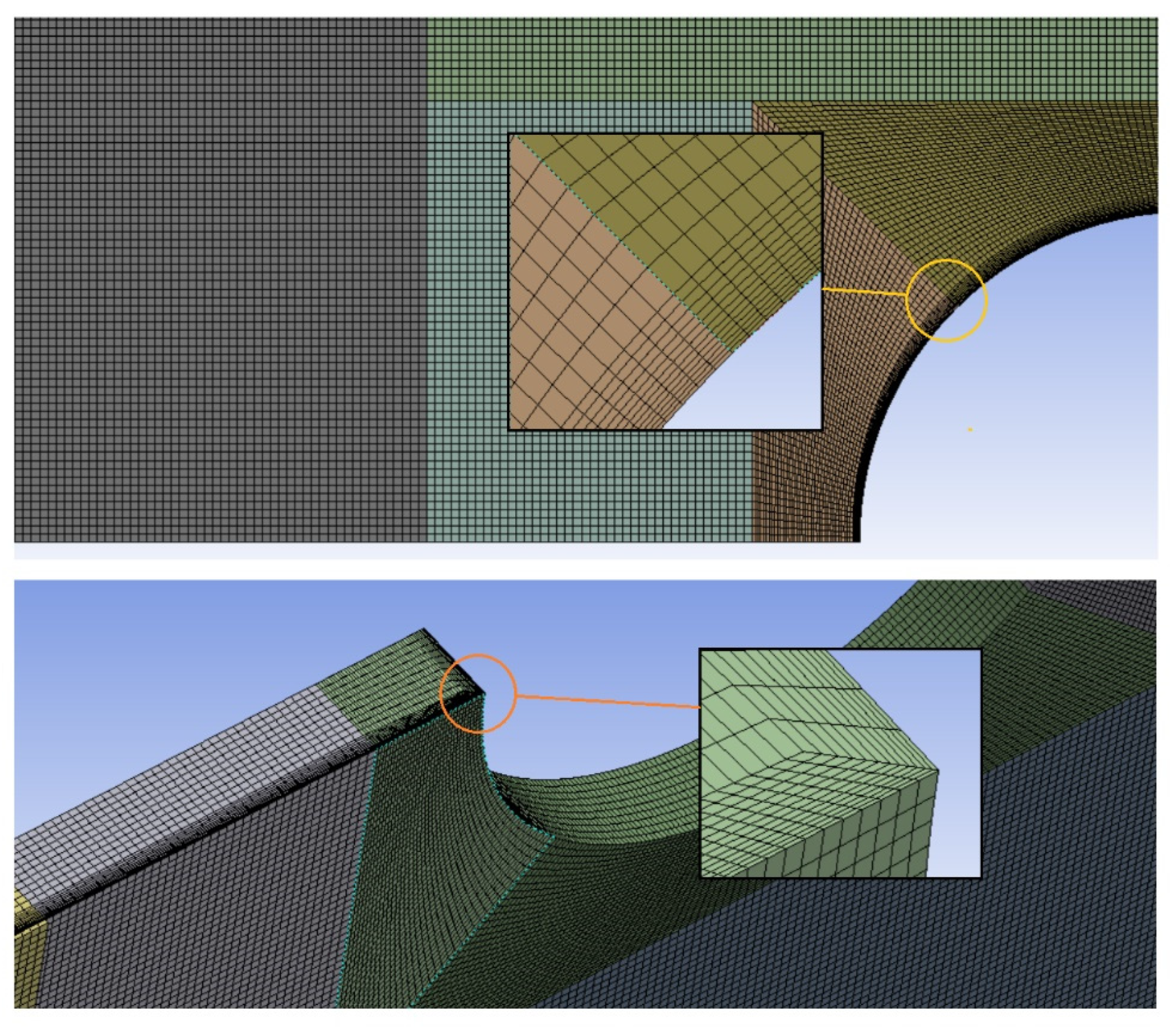
4. Mesh Parameters and Mesh Independent Study

Table 2. Mesh data for the modelled part of the heat exchanger (Figure 2).

Finite Elements Number	3,104,268
Number of nodes	3,277,429
Dimension of the element, mm	0.15
Maximum dimension of the element, mm	0.20
Boundary layer	First layer thickness: 0.023 mm $(y^{+}=1)$
	Growth rate: 1.1
	Number of layers: 12
Minimum orthogonal angle	Air: 35.6°
Mesh expansion factor	Air: 14
Maximum aspect ratio	Air: 22

presents a calculation mesh data. The calculation mesh consist of the cuboid elements only. Additionally, in order to increase accuracy of the simulations, it has densities at the boundary between the air and the fins and tubes (Figure 2). Densities are as a first layer thickness with 1.1 growth rate and 12 number of the layers.

The mesh independent study was performed for all CFD simulations for the entire range of air velocity, separately for all air velocities (Figure 3). Designation of Nusselt number stabilization was performed done by calculation of relative differences ($e_{Nu}$) between different Nusselt number in the fourth row of FHE for mesh with particular element numbers ($N{u}_n{}_i$) and the reference Nusselt number in the fourth row of PFTHE for mesh with 3,104,268 mesh elements ($N{u}_{\mathrm{3,104,268}}$) are as follows $e_{Nu}=\frac{\left(N{u}_n{}_i-N{u}_{\mathrm{3,104,268}}\right)}{N{u}_{\mathrm{3,104,268}}}$.

Nusselt number stabilisation for air velocity—10 m/s in front of the heat exchanger for the fourth row of FHE is shown in Figure 3. Acceptable Nusselt number stabilisation has been reached for mesh with 3,104,268 elements. Continuing to increase mesh elements does not provide significantly stable results and the relative differences for the mesh with the highest number elements differ less than 1.6%. The discrepancies for other rows of FHE and the lower air velocities are even close to 0. This shows that, in the considered scenario, the greatest irregularity of flow and turbulence exists in the last row of FHE.

The calculation time is also shown in Figure 3. It can be observed that the chosen mesh has more than double the calculation time compared to the mesh with the highest number of elements. The above reference mesh has been selected for further calculations as the best ratio of calculation accuracy to calculation time.

A mesh with 3,104,268 elements was selected. Mesh elements’ size belongs to the following mesh sizes: mesh element size: 0.15 mm; mesh max size: 0.20 mm (Table 2). The whole mesh contains cuboidal elements only (Figure 2).

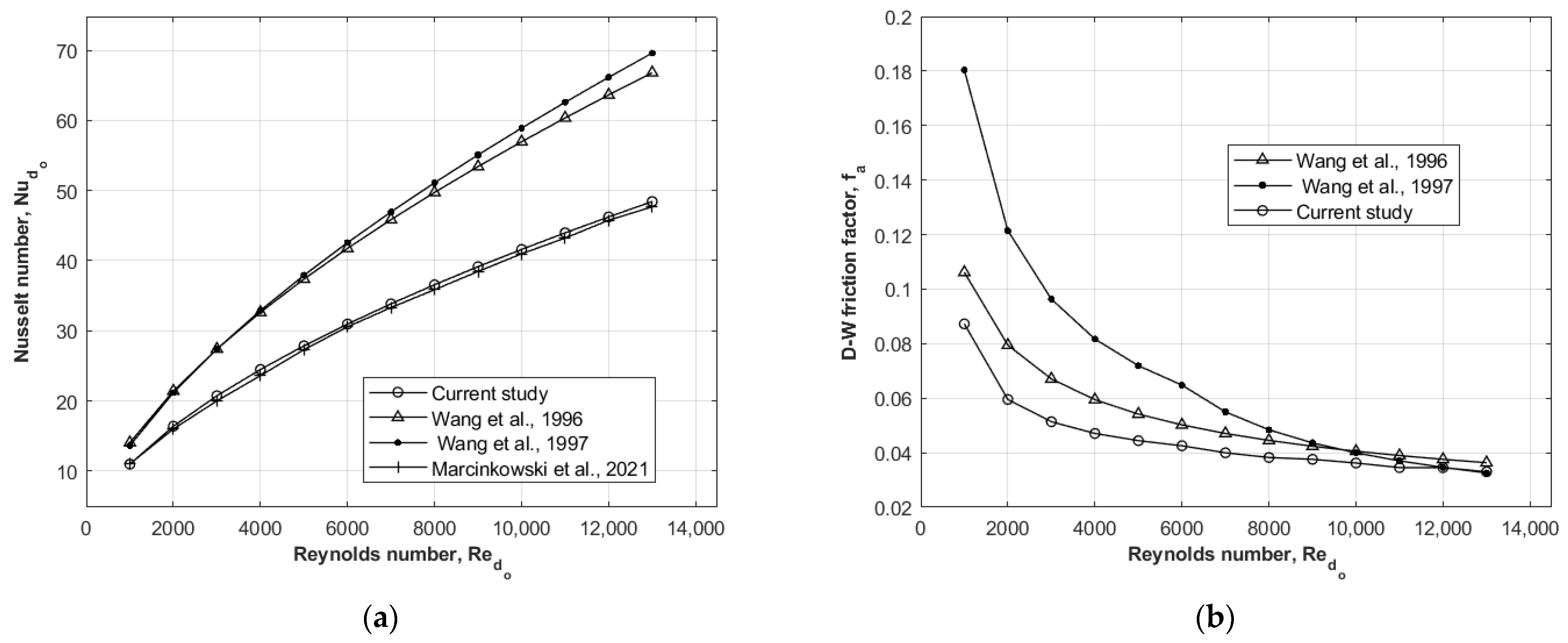
5. CFD Model Validation

Figure 4 presents the results of the Nusselt number and D-W friction factor of the currently investigated CFD model and recent correlations such as Wang et al. [28] and Wang et al. [27]. Figure 5 shows relative differences (Equation (11)) between the current study and above related research in the case of the air-side Nusselt and the air-side D-W friction factor as a function of Reynolds number.

Figure 5a compares the correlations determined by the current study with Wang et al. [28], Wang et al. [27] and Marcinkowski et al. [25] in the case of Nusselt number comparison.

Table 3. Dimensions of the FHE geometry from different research.

Description	Designation	Current Study	Wang et al. [28]	Wang et al. [27]
Rows	-	4	2–6	2–6
Transversal tube pitch [mm]	$p_t$	32.00	25.40	25.40
Longitudinal tube pitch [mm]	$p_l$	27.71	22.00	22.00
Tube outer diameter [mm]	$d_o$	12.00	10.23	10.23
Fin pitch [mm]	$s$	3.00	1.75–3.21	1.82–3.20
Fin thickness [mm]	${\delta }_f$	0.14	0.13–0.2	0.13
Fin length of single row [mm]	$L_f$	27.71	22.00	22.00

presents geometry dimensions and the limitations of the compared study. It can be noted that all the studies presented have a geometry which are close to each other.

The relative differences between the current study and the other correlations were defined as:

$$e_{param}^{diffCorr}=100\left(para{m}_{}^{diffCorr}-para{m}_{}^{Present}\right)/para{m}_{}^{diffCorr}$$

(11)

The superscript diffCorr indicates that it is the value of a given study: Wang et al. [28], Wang et al. [27] and Marcinkowski et al. [25]. The subscript param means the following parameters: Nu number and j-factor.

The relative difference between the Nusselt number presented in this study and the Nusselt number correlation for Wang et al. [28], is 21.87% for $R{e}_{d_o}$ = 1000 and 27.51% for $R{e}_{d_o}$ = 13,000 (Figure 5a). The relative difference between the Nusselt number presented in this study and the Nusselt number correlation for Wang et al. [27], is 19.42% for $R{e}_{d_o}$ = 1000 and 30.42% for $R{e}_{d_o}$ = 13,000 (Figure 5a). The relative difference between the Nusselt number presented in this study and the Nusselt number correlation for Marcinkowski et al. [25] is −3.6% for $R{e}_{d_o}$ = 3000, 0.33% for $R{e}_{d_o}$ = 1000 and −1.58% for $R{e}_{d_o}$ = 13,000 (Figure 5a). The results of Marcinkowski et al. [25] were performed by CFD modelling using Ansys CFX software. The current study was performed for the same mathematical model. The only difference for the range of the Nusselt number test is due to the use of Ansys Fluent.

Figure 5b compares the correlations determined by the current study with Wang et al. [28] and Wang et al. [27] in the case of D-W friction factor comparison.

The relative difference between the friction factor correlation presented in this study and the friction factor correlation for Wang et al. [28], is 17.8% for $R{e}_{d_o}$ = 1000 and 9.13% for $R{e}_{d_o}$ = 13,000 (Figure 5b). The relative difference between the friction factor correlation presented in this study and the friction factor correlation for Wang et al. [27], is 51.62% for $R{e}_{d_o}$ = 1000 and −1.29% for $R{e}_{d_o}$ = 13,000 (Figure 5b).

The above results in Figure 4 and Figure 5 show that the developed model and calculations performed in Ansys Fluent fairly accurately reproduce the heat transfer assumptions in the heat exchangers discussed. The slight differences may be due to the fact that the correlation presented in this work was determined using CFD modelling, while the other correlations were determined using experimental tests. The differences between the correlations obtained experimentally and the correlation determined by Ansys Fluent calculations are acceptable (Figure 5), given that the geometries of the exchangers analysed differ both in tube diameter and in the spacing of tubes and fin fins. Also, different experimental test conditions and the conditions adopted in the CFD modelling can cause differences in the values of the Nusselt number and the friction coefficient.

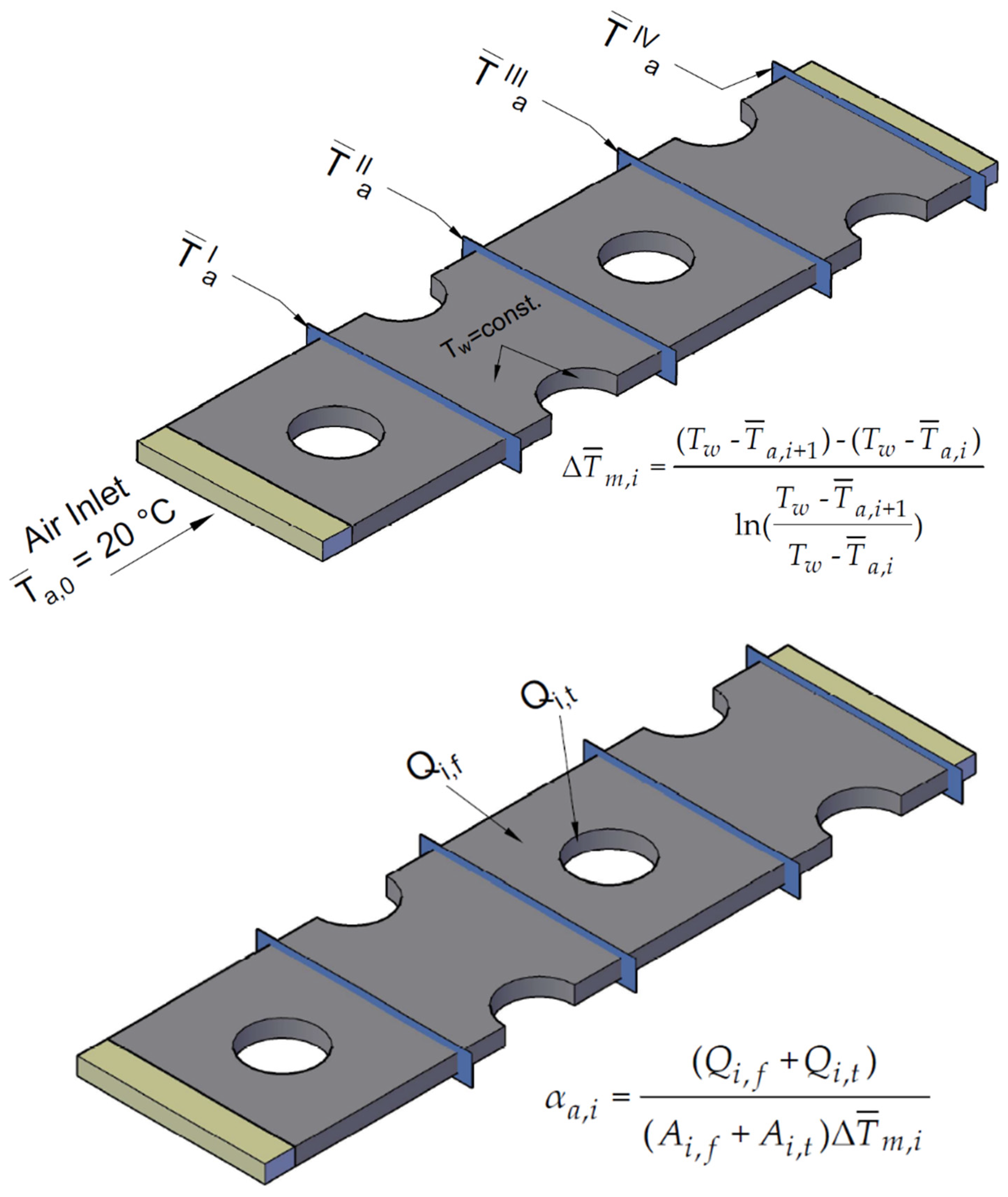
6. Method of Determining HTC on the Individual FHE Row

Determination of the HTCs for the individual rows is illustrated in Figure 6. The method uses constant fin and tube temperatures (70 °C). Previous paper of Marcinkowski et al. [25] shows also simulations for constant fin and tube temperatures: 60 °C and 80 °C. The determined HTCs do not differ more than 1.5% for different constant surface temperatures of the tubes and fins. The simplicity of this method means that it can be used in practice.

Determining HTC, Nusselt number and Colburn factor:

• Extract the average mass flow temperature ${\overline{T}}_a^i$ from the Fluent Post-Processor of the air velocity for every row separately. Areas to extract the average mass flow temperatures are in a half distance between the next two tubes in rows.
• Compute the difference of the average logarithmic temperature ($\Delta {\overline{T}}_{m,a}$) 14 between the fin and the tube surface temperature ($T_w$) and the average mass flow temperature (${\overline{T}}_a^i$) (Equation (12)).

$$\Delta {\overline{T}}_{m,a}=\frac{\left(T_w-{\overline{T}}_a^{i+1}\right)\left(T_w-{\overline{T}}_a^i\right)}{\ln \left(\frac{T_w-{\overline{T}}_a^{i+1}}{T_w-{\overline{T}}_a^i}\right)}$$

(12)

The symbol $T_w$ means the constant fin and tube surface temperature. The symbols ${\overline{T}}_a^i \mathrm{and} {\overline{T}}_a^{i+1}$ denotes the inlet and outlet mass average air temperature for the i-th row of FTHE.

• Extract the total heat flow transferred from the fin and the tube wall surface to the air for the i-th row of the FTHE (Figure 6).
• Compute the individual HTC for each row separately (Equation (13)) [14].

$${\alpha }_a^i=Q_i/\left(A_w{\Delta T}_{m,a}^i\right)$$

(13)

The symbol $Q_{ i}$ means the total heat flow for the individual row for the i-th row of the FTHE; ${\alpha }_a^i$ denotes the air-side HTC for the i-th row of the FTHE.

• Compute the Nusselt number (Equation (14)) [14].

$$N{u}_a^i=({\alpha }_a^i d_h)/{\lambda }_a$$

(14)

Determining friction factor:

• Extract the average value of static pressure $\Delta {\overline{p}}_a^{ i}$ from the Fluent CFD-Post of the air velocity for every row separately. Areas to extract the average value of the static pressure are in a half distance between the next two tubes in rows.
• Compute the individual Darcy-Weisbach friction factor for each row separately (Equation (15)) [35].

$$f_a^{ i}=\left(\frac{d_h{\overline{\rho }}_a^i}{L_r{\rho }_a^i}\right)\left[\frac{2{\rho }_a^i\Delta {\overline{p}}_a^{ i}}{{\overline{\rho }}_a^i{w}_{max}^i}-\left(1+{\sigma }^2\right)\left(\frac{{\rho }_a^i}{{\rho }_a^{i+1}}-1\right)\right]$$

(15)

The symbol $d_h$ means hydraulic diameter (Equation (8)), ${\overline{\rho }}_a^i$ denotes the arithmetic average of the air density for the i-th row of the FHE; ${\rho }_a^i$ means the inlet air density, ${\rho }_a^{i+1}$ means the inlet air density, $L_r$ designated the length of the considered volume, $w_{max}^i$ designated the maximum air velocity (Equation (9)) for the i-th row of the FHE. The other symbols mean: $\Delta {\overline{p}}_a^{ i}$ denotes the average air pressure drop for the i-th row of FHE, $\sigma$ designated ratio of the fin pitch cross section and two next fins distance cross section area.

7. Results and Discussion

Figure 7 and Figure 8 present results of Nusselt number and D-W friction factor for both individual correlation on each row and average correlations for the entire FHE. Parameter $w_{\mathit{max}}$ in Equations (7) and (8) is almost double the air velocity in front of the FHE. Reynolds numbers are related to the maximum velocity, which is why the Reynolds number for the same air velocity in front of the FHE has a different value for the maximum air velocity of the i-th tube rows of FHE.

The high value of the average Nusselt number on the first tube row for low air velocities (Figure 7a) is due to the high local values of the Nusselt number in the developing (run-up) section in channels formed by adjacent continuous fins. The influence of the dead zone in the area of the rear surface of the tube (rear stagnation point) is smaller than in the second and third rows. The smaller values of the average Nusselt number on the second and third rows of tubes are due to the formation of air vortices near the front and rear surfaces of the tube. These are dead zones from the point of view of heat transfer since the temperature of the swirling air is close to that of the fin and tube surfaces. The average Nusselt number for the fourth row of tubes is greater than the average Nusselt number on the third row of tubes for Rea > 400. This is due to the smaller surface area of the tubes and fins near which air vortices occur compared to the second and third rows.

When Reynolds numbers are greater than 1200, the distribution of the average Nusselt number on each tube row is different from that for smaller Reynolds numbers (Figure 7b). It is to be expected that the air flow in the channels formed by the fins is largely turbulent. In turbulent flows, the length of the inlet (developing) flow section where the air flow is hydraulically and thermally developed is significantly smaller compared to laminar flow. The contribution of the inlet section to raising the average Nusselt number for the first and second row of tubes is smaller than for laminar flow. The dead zones in the area of the rear surface of the first and second row of tubes are similar. Therefore, the average Nusselt numbers for the first and second row of tubes are similar. Only in the range of Reynolds numbers from 1200 to 3200, the average Nusselt number on the first row is larger than on the second row of tubes. This is due to the larger value of the average Nusselt number on the inlet (developing) flow section for the first row of tubes for smaller Reynolds numbers compared to the average value of the Nusselt number on the inlet section in front of the second row of tubes. The front and rear stagnation point area on the third tube row has large dead zones from a heat transfer perspective, resulting in a low value of the average Nusselt number on this row. The high value of the average Nusselt number on the fourth tube row is due to the smaller dead zone area close to the rear stagnation point area behind the fourth tube row.

The Nusselt number function which was approximate to the modelled CFD data is presented in Equation (16). This function contains two parameters: $x_1$ and $x_2$, which was presented in

Table 4. Air side Nusselt number correlation parameters of FTHE for Reynolds number range from 150 to 1400.

	Nusselt Number Correlations	Friction Factor Correlations
Average	$N{u}_a=0.9760 R{e}_a^{0.3337} P{r}_a^{1/3}$	$f_a=1.3788 R{e}_a^{-0.4569}$
Row 1	$N{u}_a=1.4001 R{e}_a^{0.3053} P{r}_a^{1/3}$	$f_a=1.3051 R{e}_a^{-0.4028}$
Row 2	$N{u}_a=0.9478 R{e}_a^{0.3386} P{r}_a^{1/3}$	$f_a=1.0700 R{e}_a^{-0.4305}$
Row 3	$N{u}_a=1.0403 R{e}_a^{0.3025} P{r}_a^{1/3}$	$f_a=1.4770 R{e}_a^{-0.5010}$
Row 4	$N{u}_a=0.5230 R{e}_a^{0.4156} P{r}_a^{1/3}$	$f_a=0.9585 R{e}_a^{-0.4249}$

and

Table 5. Air side Nusselt number correlation parameters of FTHE for Reynolds number range from 1400 to 6000.

	Nusselt Number Correlations	Friction Factor Correlations
Average	$N{u}_a=0.1652 R{e}_a^{0.5781} P{r}_a^{1/3}$	$f_a=0.2673 R{e}_a^{-0.2251}$
Row 1	$N{u}_a=0.4217 R{e}_a^{0.4700} P{r}_a^{1/3}$	$f_a=0.3370 R{e}_a^{-0.2127}$
Row 2	$N{u}_a=0.1305 R{e}_a^{0.6118} P{r}_a^{1/3}$	$f_a=0.1983 R{e}_a^{-0.1917}$
Row 3	$N{u}_a=0.0923 R{e}_a^{0.6307} P{r}_a^{1/3}$	$f_a=0.3523 R{e}_a^{-0.3006}$
Row 4	$N{u}_a=0.1282 R{e}_a^{0.6145} P{r}_a^{1/3}$	$f_a=0.2303 R{e}_a^{-0.2173}$

. The function depends on the Reynolds number based on the hydraulic diameter (Equation (10)) and Prandl number. Equation (16) presents also a range of Reynolds number and Prandtl number range.

$$N{u}_a=x_1\cdot {\mathit{Re}}_a^{x_2}\cdot P{r}_a^{\frac{1}{3}}\hspace{1em}\hspace{1em}\hspace{1em}\hspace{1em}\hspace{1em}\hspace{1em}150\le {\mathit{Re}}_a\le 5900, P{r}_a=0.7$$

(16)

The air-side Nusselt number (${\mathit{Nu}}_a$) correlation (Equation (16)) follows the Colburn relation $Nu/\left(ReP{r}^{1/3}\right)=f\left(Re\right)$ where the function f (Re) is determined using experimental data. Having determined the coefficients ×1 and ×2 for the air-side Nusselt number function (Equation (9)) by means of CFD modelling, it can be expected that the function (Equation (16)) will also be valid for other gases. The Nusselt numbers functions for the first, second, third, fourth rows of tubes and the average Nusselt numbers function for the entire FTHE are illustrated in Figure 7. Table 4 and Table 5 show the corresponding correlation’s parameters for all functions presented in Figure 7.

The D-W friction factor function which was approximate to the modelled CFD data is presented in the Equation (17). The friction factor function contains two parameters: $x_1$ and $x_2$, which was presented in Table 4 and Table 5. The function depends on the Reynolds number and Prandl number. Equation (17) presents also range of Reynolds number.

$$f_a=x_1\cdot {\mathit{Re}}_a^{x_2}\hspace{1em}\hspace{1em}\hspace{1em}\hspace{1em}\hspace{1em}\hspace{1em}{\mathit{Re}}_a=\frac{w_{\mathit{max}}{d}_h}{{\nu }_a},150\le {\mathit{Re}}_a\le 5900$$

(17)

The friction factor functions for the first, second, third, fourth rows of tubes and the average friction factor function for the entire FTHE are illustrated in Figure 8. Table 4 and Table 5 show the corresponding correlation’s parameters for all functions presented in Figure 8.

The coefficients x₁ and x₂ for each correlation was calculated considering the 95% confidence interval limits for the Nusselt numbers which are determined by the least-squares method. The values of the Nusselt number (Equation (14)) calculated for a given Reynolds number (Equation (10)) differ by +/− 2 σ. The σ symbol means the mean standard deviation of the Nusselt numbers obtained by the CFD modelling. The determination of 95% confidence intervals for Nusselt number correlations received by least-squares is described at Chapter 11 of Taler’s book [24].

8. Conclusions

The new air-side correlations of the Nusselt number and the D-W friction factor were proposed for the four-row FHE. The individual correlations on the individual rows of the FHE can significantly improve a construction of the FHEs. This paper presented the analysed range of the air velocities in the front of the heat exchanger from 0.5 m/s to 10 m/s. Both the Nusselt number correlations and the D-W friction factors for modelled FHE were developed using the CFD software–Ansys 2020 R2 Fluent. The newly determined individual correlations (Table 4 and Table 5) for dedicated rows are considerably different from the average correlations of the Nusselt numbers and the D-W friction factors (Figure 7 and Figure 8). The conclusions are as follows:

• The results of the comparison the current average Nusselt number correlations for the entire FHE with author’s previous average Nusselt number correlations for the entire FHE are almost identical. The relative differences for the entire Reynolds number range from 200 to 6000 is maximum 3.6% (Figure 5). The important information is that the current data were calculated using Ansys 2020 R2 Fluent software, whereas the previous author’s data were determined using Ansys 2020 R2 CFX software.
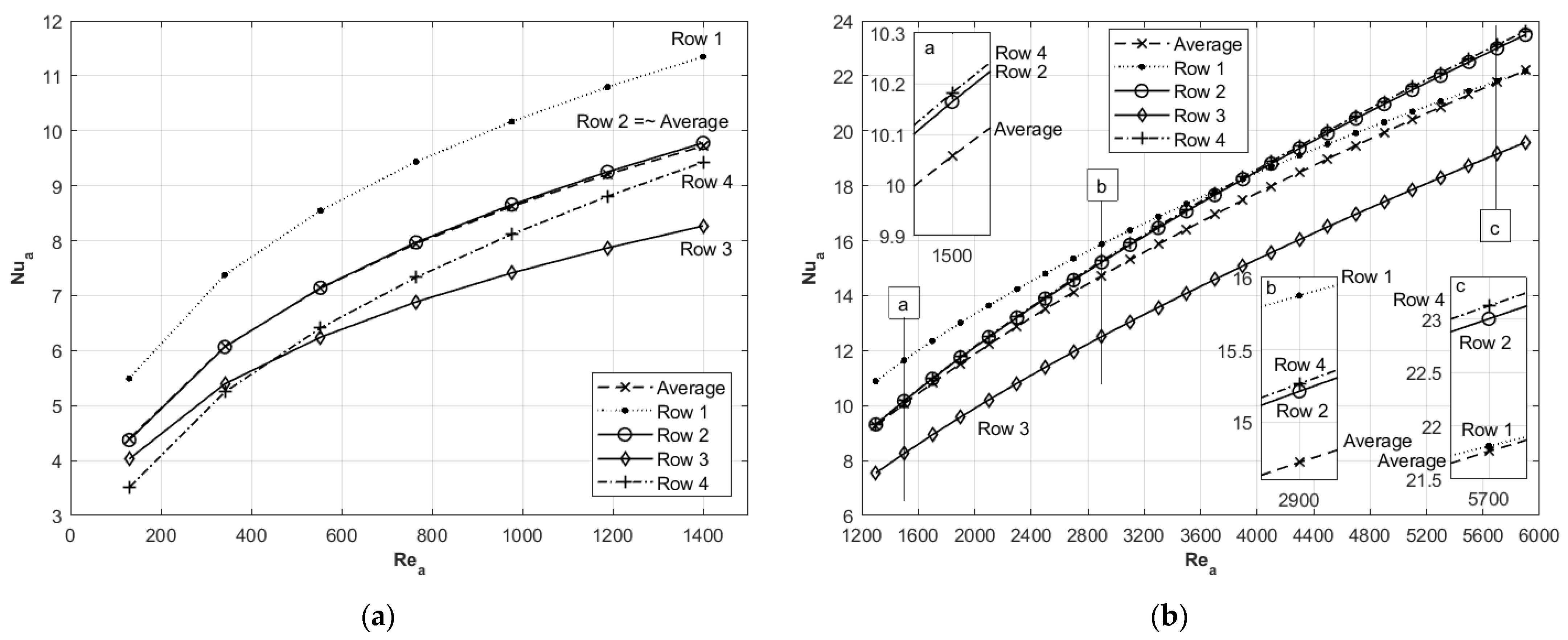
• The obtained Nusselt numbers and D-W friction factors data are the highest value for the first row of the FHE for Reynolds number ranging from 200 to 6000, due to the maximum temperature difference between air and heat transfer surface (fin and tubes). The fewest dead zones exist also in the first row of tubes (Figure 7 and Figure 8).
• The obtained Nusselt number and friction factors correlations showed that the third row is the least efficient for Reynolds number ranging from 200 to 6000, because the third row is the least turbulent and air stream develops a narrow flow channel. The rest of the volume creates broad dead zones in front of and behind the tubes in the third row (Figure 7 and Figure 8).
• The greater the Reynolds number for the range tested, the more the Nusselt number values for the first row converge to the average value for the entire FHE. Moreover, the higher the Reynolds number for the range tested, the more the Nusselt values for the second- and the third-row values equalise and increase from the mean value for the entire FHE (Figure 7).
• The research also showed the clear and accessible method for the determination of the Nusselt number and friction factor correlation for individual rows which can reduce or even completely eliminate expensive experimental research (Figure 6).
• The presented method (Figure 6) can be used not only for designing coolers and heaters in air-conditioning or other finned heat exchangers in heat recovery, but also for evaporators and condensers in air heat pump, cooling, and refrigeration process.

The average air side Nusselt number correlations of the entire FHE are still widely used in engineering. The analytical methods which are being used to design FHE are also reference to the average value of air side Nusselt number. However, there are a couple of visible improvements in the methods for calculating FHE, especially if you consider individual air side Nusselt numbers in each row of tubes. This paper showed that thermal and hydraulic flow in FHE are complicated phenomena and the above conclusions explain a couple of them, but there is still place for more research and for sure experimental verifications.

References

- McQuistion, F.C.; Parker, J.D.; Spitler, J. Heating, Ventilating, and Air Conditioning Analysis and Design, 6th ed.; JohnWiley & Sons: Hoboken, NJ, USA, 2005. [Google Scholar]
- Menegazzo, D.; Lombardo, G.; Bobbo, S.; De Carli, M.; Fedele, L. State of the Art, Perspective and Obstacles of Ground-Source Heat Pump Technology in the European Building Sector: A Review. Energies 2022, 15, 2685. [Google Scholar] [CrossRef]
- Marina, A.; Spoelstra, S.; Zondag, H.A.; Wemmers, A.K. An estimation of the European industrial heat pump market potential. Renew. Sustain. Energy Rev. 2021, 139, 110545. [Google Scholar] [CrossRef]
- Moon, H.; McGregor, D.J.; Miljkovic, N.; King, W.P. Ultra-power-dense heat exchanger development through genetic algorithm design and additive manufacturing. Joule 2021, 5, 3045–3056. [Google Scholar] [CrossRef]
- Guo, X.; Wei, H.; He, X.; Du, J.; Yang, D. Experimental evaluation of an earth–to–air heat exchanger and air source heat pump hybrid indoor air conditioning system. Energy Build. 2022, 256, 111752. [Google Scholar]
- Wang, W.; Jiang, J.; Hu, B.; Wang, R.Z.; Luo, M.; Zhang, G.; Xiang, B. Performance improvement of air-source heat pump heating system with variable water temperature difference. Appl. Therm. Eng. 2022, 210, 118366. [Google Scholar] [CrossRef]
- Yang, T.; King, W.P.; Miljkovic, N. Phase change material-based thermal energy storage. Cell Rep. Phys. Sci. 2021, 2, 100540. [Google Scholar] [CrossRef]
- Du, K.; Calautit, J.; Eames, P.; Wu, Y. A state-of-the-art review of the application of phase change materials (PCM) in Mobilized-Thermal Energy Storage (M-TES) for recovering low-temperature industrial waste heat (IWH) for distributed heat supply. Renew. Energy 2021, 168, 1040–1057. [Google Scholar] [CrossRef]
- Najim, F.T.; Mohammed, H.I.; Taqi Al-Najjar, H.M.; Thangavelu, L.; Mahmoud, M.Z.; Mahdi, J.M.; Tiji, M.E.; Yaïci, W.; Talebizadehsardari, P. Improved Melting of Latent Heat Storage Using Fin Arrays with Non-Uniform Dimensions and Distinct Patterns. Nanomaterials 2022, 12, 403. [Google Scholar] [CrossRef] [PubMed]
- Mahdi, J.M.; Najim, F.T.; Aljubury, I.M.A.; Mohammed, H.I.; Khedher, N.B.; Alshammari, N.K.; Cairns, A.; Talebizadehsardari, P. Intensifying the thermal response of PCM via fin-assisted foam strips in the shell-and-tube heat storage system. J. Energy Storage 2022, 45, 103733. [Google Scholar] [CrossRef]
- Sun, X.; Mohammed, H.I.; Tiji, M.E.; Mahdi, J.M.; Majdi, H.S.; Wang, Z.; Talebizadehsardari, P.; Yaïci, W. Investigation of Heat Transfer Enhancement in a Triple Tube Latent Heat Storage System Using Circular Fins with Inline and Staggered Arrangements. Nanomaterials 2021, 11, 2647. [Google Scholar] [CrossRef] [PubMed]
- Rao, R.V.; Saroj, A.; Ocloń, P.; Taler, J. Design Optimization of Heat Exchangers with Advanced Optimization Techniques: A Review. Arch. Comput. Methods Eng. 2019, 27, 517–548. [Google Scholar] [CrossRef]
- Taler, D.; Taler, J.; Trojan, M. Thermal calculations of plate–fin–and-tube heat exchangers with different heat transfer coefficients on each tube row. Energy 2020, 203, 117806. [Google Scholar] [CrossRef]
- Thulukkanam, K. Heat Exchanger Design Handbook, 2nd ed.; CRC Press: Boca Raton, FL, USA, 2013. [Google Scholar]
- Bošnjaković, M.; Muhič, S. Numerical Analysis of Tube Heat Exchanger with Trimmed Star-Shaped Fins. Appl. Sci. 2022, 12, 4857. [Google Scholar] [CrossRef]
- Hassan, M.; Mebarek-Oudina, F.; Faisal, A.; Ghafar, A.; Ismail, A.I. Thermal energy and mass transport of shear thinning fluid under effects of low to high shear rate viscosity. Int. J. Thermofluids 2022, 15, 100176. [Google Scholar] [CrossRef]
- Sadeghianjahromi, A.; Wang, C.C. Heat transfer enhancement in fin-and-tube heat exchangers—A review on different mechanisms. Renew. Sustain. Energy Rev. 2021, 137, 110470. [Google Scholar] [CrossRef]
- Zhang, J.; Liu, J.; Zhang, L.; Liu, Q.; Wu, Q. Air-side heat transfer characteristics under wet conditions at lower ambient pressure of fin-and-tube heat exchanger. Int. J. Heat Mass Transf. 2019, 142, 118439. [Google Scholar] [CrossRef]
- Jige, D.; Sugihara, K.; Inoue, N. Evaporation heat transfer and flow characteristics of vertical upward flow in a plate-fin heat exchanger. Int. J. Refrig. 2022, 133, 165–171. [Google Scholar] [CrossRef]
- Vaisi, A.; Javaherdeh, K.; Moosavi, R. Condensation heat transfer performance in multi-fluid compact heat exchangers with wavy and strip fins. Int. J. Heat Mass Transf. 2022, 182, 121968. [Google Scholar] [CrossRef]
- Xie, G.; Wang, Q.; Sunden, B. Parametric study and multiple correlations on air-side heat transfer and friction characteristics of fin-and-tube heat exchangers with large number of large-diameter tube rows. Appl. Therm. Eng. 2008, 29, 1–16. [Google Scholar] [CrossRef] [Green Version]
- Kim, Y.; Kim, Y. Heat transfer characteristics of flat plate finned-tube heat exchangers with large fin pitch. Int. J. Refrig. 2005, 28, 851–858. [Google Scholar] [CrossRef]
- Che, M.; Elbel, S. Comparison of Local and Averaged Air-Side Heat Transfer Coefficients on Fin-and-Tube Heat Exchangers Obtained With Experimental and Numerical Methods. J. Therm. Sci. Eng. Appl. 2022, 14, 071013. [Google Scholar] [CrossRef]
- Węglarz, K.; Taler, D.; Jaremkiewicz, M.; Taler, J.; Marcinkowski, M. Analytical-numerical method for calculating cross-flow tube heat exchangers considering temperature-dependent fluid heat capacities. Int. J. Heat Mass Transf. 2022, 183, 122202. [Google Scholar] [CrossRef]
- Marcinkowski, M.; Taler, D.; Taler, J.; Węglarz, K. Thermal Calculations of Four-Row Plate-Fin and Tube Heat Exchanger Taking into Account Different Air-Side Correlations on Individual Rows of Tubes for Low Reynold Numbers. Energies 2021, 14, 6978. [Google Scholar] [CrossRef]
- Kelvion. Compact Fin and Tube Coils. Available online: https://www.kelvion.com/products/product/coils/ (accessed on 26 June 2022).
- Wang, C.C.; Hsieh, Y.C.; Lin, Y.T. Performance of Plate Finned Tube Heat Exchangers Under Dehumidifying Conditions. J. Heat Transf. 1997, 119, 109–117. [Google Scholar] [CrossRef]
- Wang, C.C.; Chang, Y.J.; Hsieh, Y.C.; Lin, Y.T. Sensible heat and friction characteristics of plate fin-and-tube heat exchangers having plane fins. Int. J. Refrig. 1996, 19, 223–230. [Google Scholar] [CrossRef]
- Li, H.; Zhang, S.; Ji, Y.; Sun, M.; Li, X.; Sheng, Y. The influence of catchment scale on comprehensive heat transfer performance about tube fin heat exchanger in numerical calculation. Energy Rep. 2022, 8, 147–155. [Google Scholar] [CrossRef]
- Menéndez Pérez, A.; Fernández-Aballí Altamirano, C.; Borrajo Pérez, R. Parametric analysis of the influence of geometric variables of vortex generators on compact louver fin heat exchangers. Therm. Sci. Eng. Prog. 2021, 27, 101151. [Google Scholar] [CrossRef]
- Zeeshan, M.; Nath, S.; Bhanja, D. Numerical study to predict optimal configuration of fin and tube compact heat exchanger with various tube shapes and spatial arrangements. Energy Convers. Manag. 2017, 148, 737–752. [Google Scholar] [CrossRef]
- Zhao, L.; Gu, X.; Gao, L.; Yang, Z. Numerical study on airside thermal-hydraulic performance of rectangular finned elliptical tube heat exchanger with large row number in turbulent flow regime. Int. J. Heat Mass Transf. 2017, 114, 1314–1330. [Google Scholar] [CrossRef]
- Okbaz, A.; Pınarbas, A.; Olcay, A.B.; Aksoy, H. An experimental, computational and flow visualization study on the air-side thermal and hydraulic performance of louvered fin and round tube heat exchangers. Int. J. Heat Mass Transf. 2018, 121, 153–169. [Google Scholar] [CrossRef]
- ANSYS FLUENT 12.0 Theory Guide—1.2 Continuity and Momentum Equations. Available online: https://www.afs.enea.it/project/neptunius/docs/fluent/html/th/node11.htm (accessed on 25 July 2022).
- Kays, W.; London, A. Compact Heat Exchangers, 3rd ed.; Krieger Pub Co.: Malabar, FL, USA, 1998. [Google Scholar]