Waste Heat Recovery from Air Using Porous Media and Conversion to Electricity

Abstract

This paper presents a numerical study of waste heat recovery from a fluid stream using thermoelectric devices. The system consisted of a square section duct with spherical porous media placed in its central region. Hot air circulates continuously through the duct and exchanges energy with the solid matrix and subsequently with the thermoelectric modules. The mathematical model of the system was solved using ANSYS/FLUENT software, requiring the implementation of user-defined functions (UDFs) and user-defined scalars (UDS) regarding porous media and thermoelectric generation modelling. From the simulations carried out, global efficiency and electrical power values were obtained in the range of [0.11–4.51] [%] and [0.01–12.77] [W], respectively. Furthermore, for the set of variables analysed, it was observed that the performance of the system is favoured by an increase in the fluid inlet temperature and speed, as well as by a higher external heat transfer coefficient.

1. Introduction

In recent years, there has been growing concern about issues such as pollutant emissions, climate change and the depletion of energy resources. The foregoing, together with the sustained increase in energy demand projected by the International Energy Agency (IEA) [1], has led to extensive research into the development of new technologies that are capable of providing solutions to these problems. One of them is the efficient use of the primary energy carriers of various industrial sectors by recovering a portion of the thermal energy dissipated. The amount of waste heat is usually estimated in the range 20–50 [%] of the total energy input in industries [2]; therefore, it is important to implement measures that allow reducing and/or recovering this important fraction of rejected energy. Some measures that can increase the energy efficiency of processes include proper planning of the productive process, investment in energy-efficient equipment, recycling of energy in the industrial production process and recovery of excess energy and subsequent utilisation in other processes [3]. Industrial waste heat is defined as heat rejected from industrial processes, in which energy is used to produce high-added-value products. The most common ones are gaseous streams (e.g., exhaust gas, flaring gas, low-quality steam, cooling air, etc.), liquid streams (e.g., hot oil, cooling water, etc.) and solids (e.g., commodities and products, such as hot steel) [4]. The amount of waste heat as a fraction of energy consumption greatly varies among the various industrial sectors [5]. The temperature at which the heat is available also varies within a very wide range, from about 50 [°C] up to even 1000 [°C] or higher, depending on the industrial sector and the process. The EU has a total residual heat potential of approximately 300 [TWh/year], of which one-third corresponds to the temperature level below 200 [°C], 25 [%] corresponds to the temperature range between 200–500 [°C] and the rest corresponds to the temperature level above 500 [°C] [6].

Waste heat recovery methods are still deficient, and progress through the design and implementation of innovative technology should be thoroughly investigated. Thermoelectric generation technology, as one entirely solid-state energy conversion method, can directly transform thermal energy into electricity by using thermoelectric transformation materials. A thermoelectric power converter has no moving parts, and it is compact, quiet, highly reliable and environmentally friendly [7,8]. Owing to these advantages, there have been considerable emphases on the development of a small thermoelectric generator (TEG) for a variety of aerospace and military applications. In recent years, studies on thermoelectric generation related to subjects such as industrial plants, geothermal areas, automobile engines, computers and the human body on the production of electrical energy with TEGs have focused on the recycling of waste heat [9]. More recently, there is a growing interest in waste-heat TEGs, using various heat sources such as combustion of solid waste, geothermal energy, thermal energy available in vehicles, power plants and other industrial heat-generating processes [10,11,12]. Power generation from waste heat streams using thermoelectric materials has been overlooked due to low thermal efficiencies (∼4 [%]) [13] and relatively high cost per Watt of generated power [14]. This low performance is caused by several factors, one of the most important being poor heat transfer from the waste heat source to the thermoelectric devices, which prevents the development of a higher temperature gradient between the thermoelements. This, coupled with the low operating pressures at which the waste-heat-carrying fluid streams are found (close to atmospheric), makes it even more difficult to develop a temperature difference between the ends of the device [14]. Several technologies and techniques exist to increase heat flow to TEGs, including micro- and mini-channel heat sinks, two-phase flow systems, static mixers and porous media, the latter of which have been shown to be effective in waste heat recovery [15,16,17]. In the case of waste heat thermoelectric generators, there have been many conceptual designs of a power conversion system which are potentially capable of obtaining application in this area [18,19,20,21,22,23]. Other studies involving heat transfer from a fluid carrier to thermoelectric modules for thermal-to-electrical energy conversion have focused on porous media combustion and thermoelectric generation [24,25,26,27]. Although these are reactive flow applications, they all use a porous media to enhance the rates of heat transfer to the thermoelectric modules.

As the literature review showed, industrial waste heat recovery and conversion into electricity by thermoelectric devices has been effected mainly using clear flow in pipelines, not accounting for the energetic and economic benefits that could be brought by the implementation of porous media in the heat-recuperative schemes’ subsequent conversion of heat to electrical energy. This paper presents the governing equations and details of their implementation in Fluent. CFD simulations are carried out for a waste-heat TEG in which the fluid stream is subjected to different flow configurations, with and without porous media. Temperature and voltage fields, pressure drops and system efficiencies are obtained as results. We empirically find the field variables’ trends as functions of the heat extraction in the thermoelectric modules and fluid stream velocity. Also, the relative merit of placing a porous material to enhance heat recovery is analysed. To the best of our knowledge, there is no evidence of a similar study in the literature that considers waste heat recovery in the presence of porous media with subsequent conversion to electricity through thermoelectric phenomena.

2. Materials and Methods

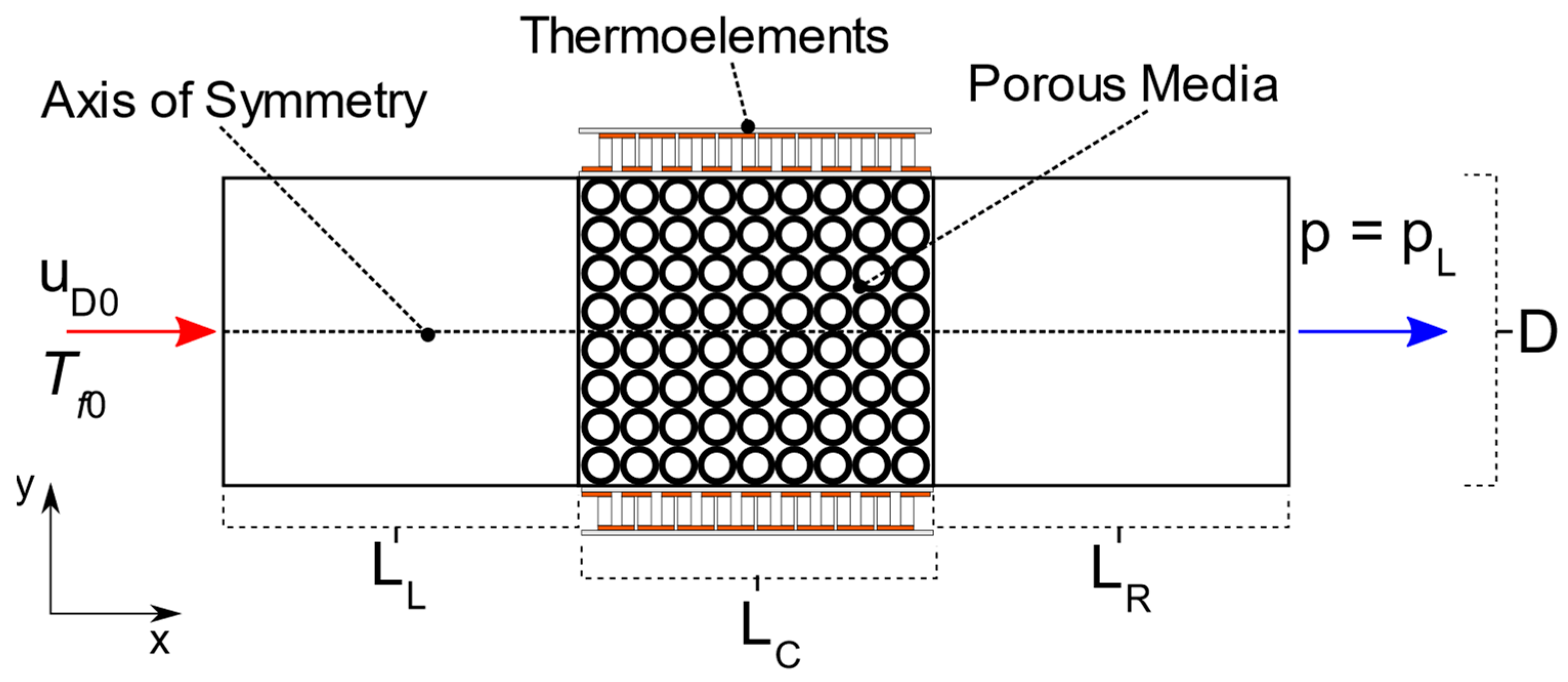
2.1. Description of the System

The physical system under study consists of a 2D duct with a square cross section of length L and side D, as shown in Figure 1. The duct is divided into three zones (L_L, L_C, L_R), and only in the central region are solid steel spheres inserted whose diameter of particle is d_p. Air enters the duct as a waste heat carrier fluid with a velocity $u_{\mathrm{D}0}$ and temperature T_f0. The selection of this working fluid was made considering the high temperatures at which it is often encountered in various applications and its extensive use in the process industry.

The walls of length L_L and L_R are considered adiabatic, while on the outside of the wall of length L_C, thermoelectric devices are arranged. These thermoelectric elements transform heat into electricity and are composed of N_n thermocouples electrically connected in series that are located between two ceramic plates. The upper ceramic plate is exposed to the environment, which has a temperature $T_{\infty }$, and thermal energy losses through a convective coefficient h are considered. This scheme allows the transfer of energy from the fluid that transports waste heat towards the thermoelectric devices, generating a potential difference due to the Seebeck effect.

Convectional thermoelectric modules consist of pairs of p-type and n-type semiconductors arranged in an alternating pattern, which are connected to each other by copper interconnecting strips, as shown in Figure 2. The heat transfer between the hot and cold sides is controlled by two plates of ceramic material, which protect the internal components of the device.

The dimensions of the waste heat recovery system are presented in

Table 1. Dimensions of the waste heat recovery system.

Symbol	Units	Value
${\mathrm{e}}_{\mathrm{Cu}}$	M	6.00 × 10−4
${\mathrm{e}}_{\mathrm{Ce}}$	M	5.00 × 10−4
${\mathrm{W}}_{\mathrm{E}}$	M	1.40 × 10−2
${\mathrm{W}}_{\mathrm{I}}$	M	1.10 × 10−3
${\mathrm{L}}_{\mathrm{Cu}}$	M	1.95 × 10−3
${\mathrm{L}}_{\mathrm{E}}$	M	1.70 × 10−3
$\mathrm{D}$	M	4.00 × 10−2
${\mathrm{L}}_{\mathrm{L}}$	M	5.00 × 10−2
${\mathrm{L}}_{\mathrm{c}}$	M	4.00 × 10−2
${\mathrm{L}}_{\mathrm{R}}$	M	5.00 × 10−2
$N_n$	[-]	16

, where the dimensions of the thermoelectric module were assigned by reference to TEC1–12706 [28,29].

2.2. Mathematical Model

2.2.1. Ideal Gas Law

The gas density was determined from the ideal gas equation for incompressible flow.

$${\rho }_f=\frac{p_0{M}_w}{R{T}_f}$$

(1)

where ${\rho }_f$ represents the density of the gas, $p_0$ is the operating pressure, $R$ is the universal gas constant, $M_w$ is the molecular weight of the gas mixture, and $T_f$ is the temperature of the gas.

2.2.2. Continuity Equation

The total mass balance for flow in porous media is given by:

$$\frac{\partial \left(\varphi {\rho }_f\right)}{\partial t}+\nabla ·\left({\rho }_f{u}_D\right)=0$$

(2)

where $\varphi$ is the porosity, $t$ is the time, and ${\mathbf{u}}_{\mathbf{D}}$ is the velocity vector.

2.2.3. Equation of Motion

Fluid momentum equation in a packed bed is given by:

$$\frac{\partial \left({\rho }_f{u}_D\right)}{\partial t}+\nabla ·\left({\rho }_f\frac{u_D u_D}{\varphi }\right)=-\varphi \nabla p+\nabla ·\left(\varphi \overline{\mathit{\tau }}\right)+\varphi {\rho }_f\mathit{g}+\varphi S_p$$

(3)

The S_p term is modelled from the Darcy–Forchheimer equation for an isotropic porous medium, as shown below [30]:

$$S_p=-\left(\frac{\mu }{K}{u}_D+C_2\frac{1}{2}{\rho }_f\left|u_D\right|u_D\right)$$

(4)

where $\mu$ represents the gas viscosity, K is the permeability, and $C_2$ is the inertial drag coefficient. These two last parameters were computed from the Ergun equation [30,31,32] using the following expressions:

$$K=\frac{d_p^2{\varphi }^3}{150{\left(1-\varphi \right)}^2}, C_2=\frac{3.5\left(1-\varphi \right)}{d_p{\varphi }^2}$$

(5)

2.2.4. Energy Equations

For the study of heat transfer in the central region of the system, a non-thermal equilibrium model was applied, characterised by an energy equation for each of the phases [30].

$$\frac{\partial \left(\varphi {\rho }_f{C}_{pf}{T}_f\right)}{\partial t}+\nabla ·\left({\rho }_f{u}_D{C}_{pf}{T}_f\right)=\nabla ·\left(\varphi {\lambda }_f·\nabla T_f\right)+h_i{a}_i\left(T_s-T_f\right)$$

(6)

$$\frac{\partial \left(\left(1-\varphi \right){\rho }_s{C}_{ps}{T}_s\right)}{\partial t}=\nabla ·\left(\left(1-\varphi \right){\mathbf{\lambda }}_s·\nabla T_s\right)-h_i{a}_i\left(T_f-T_s\right)$$

(7)

where $C_{pf}$ is the heat capacity of the fluid, ${\mathbf{\lambda }}_f$ is the thermal conductivity tensor of the gas phase, $h_i$ is the interfacial heat transfer coefficient, $a_i$ is the area per unit volume, ${\rho }_s$ is the density, $C_{ps}$ is the heat capacity, and ${\mathbf{\lambda }}_s$ is the thermal conductivity for the solid phase.

The heat transfer coefficient and interfacial areal density were obtained from the following expressions [33]:

$$h_i=\frac{{\lambda }_f}{d_p}\left(2+1.1 R{e}_p{}^{0.6} P{r}^{\frac{1}{3}}\right), a_i=\frac{6}{d_p}\left(1-\varphi \right)$$

(8)

with $d_p$ being the pore diameter, ${Re}_p$ being the particle Reynolds number and Pr being the Prandtl number.

2.2.5. Physical Properties

The physical properties of the air were computed with the following correlations [34]:

$$C_{pf}=947e^{1.83\times {10}^{-4}{T}_f}, {\lambda }_f=4.82\times {10}^{-7}{C}_{pf}{T}_f^{0.7}, \mu =3.37\times {10}^{-7}{T}_f^{0.7}.$$

(9)

2.2.6. Thermoelectric Generation

The thermogeneration model solved in the thermoelectric devices is based on the work of Antononova and Looman [35], which includes solving the equations of conservation of energy and electric charge.

$$\frac{\partial \left({\rho }_E{C}_{pE}{T}_E\right)}{\partial t}+\nabla ·\mathit{q}=\dot{q}$$

(10)

$$\nabla ·\left(\mathit{J}+\frac{\partial \mathit{D}}{\partial t}\right)=0$$

(11)

where ρ_E is the electrical conductor density, C_pE is the electrical conductor heat capacity, T_E is the electrical conductor temperature, q is the heat flux vector, $\dot{q}$ is the Joule heating source term, J is the electric current density, and D is the electric flux density.

Both equations are coupled to each other through the constitutive relations:

$$\mathit{q}=\pi \mathit{J}-{\mathbf{\lambda }}_E·\nabla T$$

(12)

$$\mathit{J}={\sigma }_E·\left(\mathit{E}-{\mathit{\alpha }}_E·\nabla T_E\right)$$

(13)

$$\mathit{D}=\mathit{\xi }·\mathit{E}$$

(14)

$$\dot{q}=\frac{{\mathit{J}}^2}{{\mathit{\sigma }}_E}$$

(15)

where ξ is the permittivity tensor, E is the electric field vector, and σ_Eis the electrical conductivity of the conductor.

In the absence of time-varying magnetic fields, the electric field is irrotational and can be derived from a scalar potential as shown below:

$$\mathit{E}=-\nabla \psi$$

(16)

Combining the equations for conservation of energy and electric charge with the constitutive relations and the expression for the electric field results in Equations (17) and (18).

$$\frac{\partial \left({\rho }_E{C}_{PE}{T}_E\right)}{\partial t}=\nabla ·\left[\left({\mathit{\sigma }}_E·{\mathit{\alpha }}_E^2{T}_E+{\mathit{\lambda }}_E\right)·\nabla T_E\right]+{\sigma }_E·\left[\left(\nabla {\psi }^2\right)+2{\mathit{\alpha }}_E·\nabla T_E·\nabla \psi +\left({\mathit{\alpha }}_E·\nabla T_E\right)\right]+\nabla ·\left({\mathit{\sigma }}_E·{\mathit{\alpha }}_E{T}_E·\nabla \psi \right)$$

(17)

$$\nabla ·\left(\mathit{\xi }·\nabla \frac{\partial \psi }{\partial t}\right)+\nabla ·\left({\mathit{\sigma }}_E·{\mathit{\alpha }}_E·\nabla T\right)+\nabla ·\left({\mathit{\sigma }}_E·\nabla \psi \right)=0$$

(18)

Figure 3 shows a set of thermocouples electrically connected in series which are arranged inside a conventional thermoelectric device. Each of these elements operates between high- and low-temperature reservoirs, where $Q_H$ and $Q_C$ represent the respective heat fluxes. The electrical current generated by the device was determined from the use of the extended Ohm’s law, as shown in the following equation:

$$I=\frac{{\alpha }_p{{\displaystyle \sum }}_{i=1}^{N_n}\Delta T_{p,i}-{\alpha }_n{{\displaystyle \sum }}_{i=1}^{N_n}\Delta T_{n,i}}{\left(1+R_{e,o}^{\ast }\right){{\displaystyle \sum }}_{i=1}^{N_n}{R}_{e,i}}$$

(19)

where $\Delta T_p$ and $\Delta T_n$ are the temperature differences between the p-type and n-type semiconductors, respectively. $R_{e,I}$ is the internal electrical resistance, and $R_{e,o}^{\ast }$ is the ratio between the external and internal electrical resistance. It is important to note that the maximum output current for Equation (19) is obtained with a value of $R_{e,o}^{\ast }=1$.

The overall efficiency of the system was determined from the ratio between the power generated by the thermoelectric device and the sensible heat given up by the fluid in the central region, which can be written as:

$$\eta =\frac{P}{Q}=\frac{I^2{N}_n{R}_{e,i}\left(1+R_{e,o}^{\ast }\right)}{{\dot{m}}_f{\overline{C}}_{pf}\left(T_{f0}-T_{f\mathrm{L}}\right)}$$

(20)

where the subscripts 0 and L represent the inlet and outlet conditions of the duct, respectively. On the other hand, expressing Equation (20) in terms of the inlet velocity of the fluid yields:

$$\eta =\frac{I^2{N}_n{R}_{e,i}\left(1+R_{e,o}^{\ast }\right)}{{\rho }_{f0}{u}_{D0}{D}^2{\overline{C}}_{pf}\left(T_{f0}-T_{f\mathrm{L}}\right)}$$

(21)

2.3. Boundary Conditions

At the duct inlet, the temperature and gas velocity were set as boundary conditions:

$$u_{\mathrm{D}}=u_{\mathrm{D}0};T_f=T_{f0}$$

(22)

At the duct outlet, the pressure of the system was specified as the atmospheric pressure, and zero gradients are set for the rest of the flow variables.

$$\nabla T_f=\nabla u_{\mathrm{D}}=0;p=p_{\mathrm{L}}$$

(23)

A no-slip condition was established at the solid–fluid interfaces. With respect to the thermoelectric device, a convective condition was set on the top wall of the device to analyse the effect of cold-side heat transfer on the performance of the system. Meanwhile, zero electric potential and the electric current density flux computed from Equation (19) were specified as boundary conditions.

$${\mathbf{\lambda }}_{cer}·\nabla T_{cer}=h(T_{cer}-T_{\infty })$$

(24)

$$\psi =0;\mathit{J}={\mathit{J}}_n$$

(25)

2.4. Simulation Conditions and Parameters

One of the problems faced by waste heat recovery system is to define the optimal operating conditions that guarantee their economic feasibility. In order to narrow down this search, the porous medium was designed taking as a reference the best results obtained by Henríquez in his study of waste heat recovery through porous media [37]. Therefore, the medium used in the simulations is a spherical steel porous medium with a porosity ϕ = 0.26 and a particle diameter d_p = 8.0 × 10⁻³ [m]. Furthermore, a temperature of 300 [K] and a pressure of 101.325 [kPa] were considered for the surrounding media in all the cases studied. Finally, different values of gas inlet velocity u_D0 = [0.5; 1.0; 1.5] [m·s⁻¹], inlet temperatures $T_{f0}=\left[350;400;450;500;550\right]$ [K] and two conditions of heat extraction rates in the central zone of the system were studied: $h_1=20$ [W·m⁻²·K⁻¹], which is a typical value of free convection of gases, and $h_2=2000$ [W·m⁻²·K⁻¹], corresponding to forced convection.

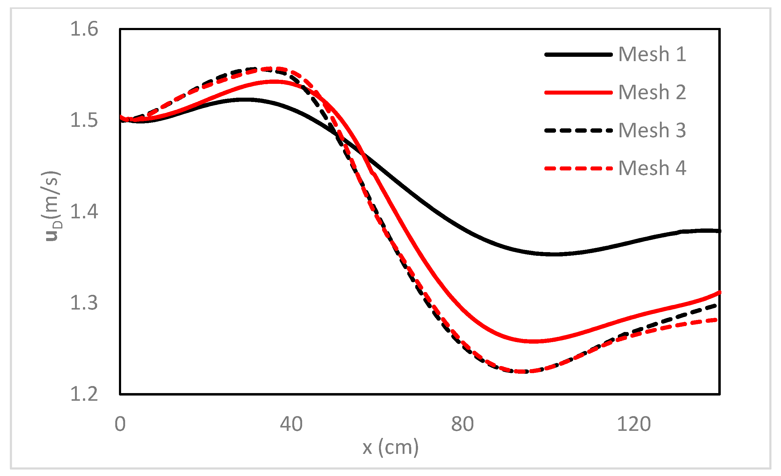
2.5. Numerical Grid Independence Test

In order to find a suitable meshing, a mesh independence test was carried out, which compared the axial velocity profiles of four meshes with different resolutions, whose properties are shown in

Table 2. Mesh properties.

Property	Mesh 1	Mesh 2	Mesh 3	Mesh 4
Element size (m)	1.00 × 10−3	6.00 × 10−4	3.00 × 10−4	1.00 × 10−4
Total number of elements	2975	8039	32,750	291,552

. For these, the conditions of higher velocity, temperature and heat dissipation coefficient were studied because these are the factors that generate the most instability in the numerical solution. From the results shown in Figure 4, it can be seen that there is little discrepancy between Mesh 3 and Mesh 4; thus, an element size of 3.00 × 10⁻⁴ [m] was used. The mesh quality was analysed by means of two metrics: the first one is the skewness, which takes a maximum value of 0.5 and an average value of 4.5 × 10⁻³; the second is the orthogonal quality metric, for which a minimum value of 0.7 with an average value of 0.99 was obtained.

2.6. Numerical Method

Because the FLUENT interface does not cover all the modelling needs of the user, it provides two extensions to implement additional aspects to those that the software has by default. The first of these is the user-defined functions (UDFs), which is a set of routines written in the C language that allows customising aspects such as: edge conditions, source terms, reaction rates, physical properties, etc. In the present article, the UDFs are programmed to define the source terms of Equation (17) and (18), to modify the physical properties of the fluid and to define the interfacial heat transfer coefficient in the porous region.

The second extension is the user-defined scalars (UDS), which allow the solving of transport equations for some arbitrary scalar. In this article, they were used to incorporate the electric charge conservation equation, as well as to define the derivatives of the flow variables to be solved in the thermogeneration model. These transport equations have the following form [11]:

$$\frac{\partial \left(\rho \phi \right)}{\partial t}+\nabla ·\left(\rho u_{\mathrm{D}}\varphi -\mathit{\Gamma }·\nabla \phi \right)=S$$

(26)

where $\mathit{\Gamma }$ and $S$ are the diffusion tensor and source term, respectively, which must be defined for each scalar equation.

Given the complexity of the phenomenon studied, the model was solved using plane-axial symmetry. The system of differential equations was discretised using the finite volume method (FVM), employing a PRESTO scheme to approximate the pressure values at the faces, while second-order upwind schemes were used to approximate the convective terms of the rest of the flow variables. Under-relaxation factors of 0.5 were used for the equation of motion and 0.7 for the rest of the transport equations. Finally, the pressure–velocity coupling was solved using the SIMPLE algorithm for incompressible fluids [38].

Thermoelectricity model validation was conducted, replicating the results of Jaegle [39] and by the authors in a previous publication [27]. Both in thermoelectricity model validation and in the computations of this investigation, the physical properties of the semiconductor material (bismuth telluride) and the copper electrodes independent of temperature were considered. On the other hand, the transport in porous media model was studied and validated by the authors, who presented their results in previous scientific articles [24,25,26].

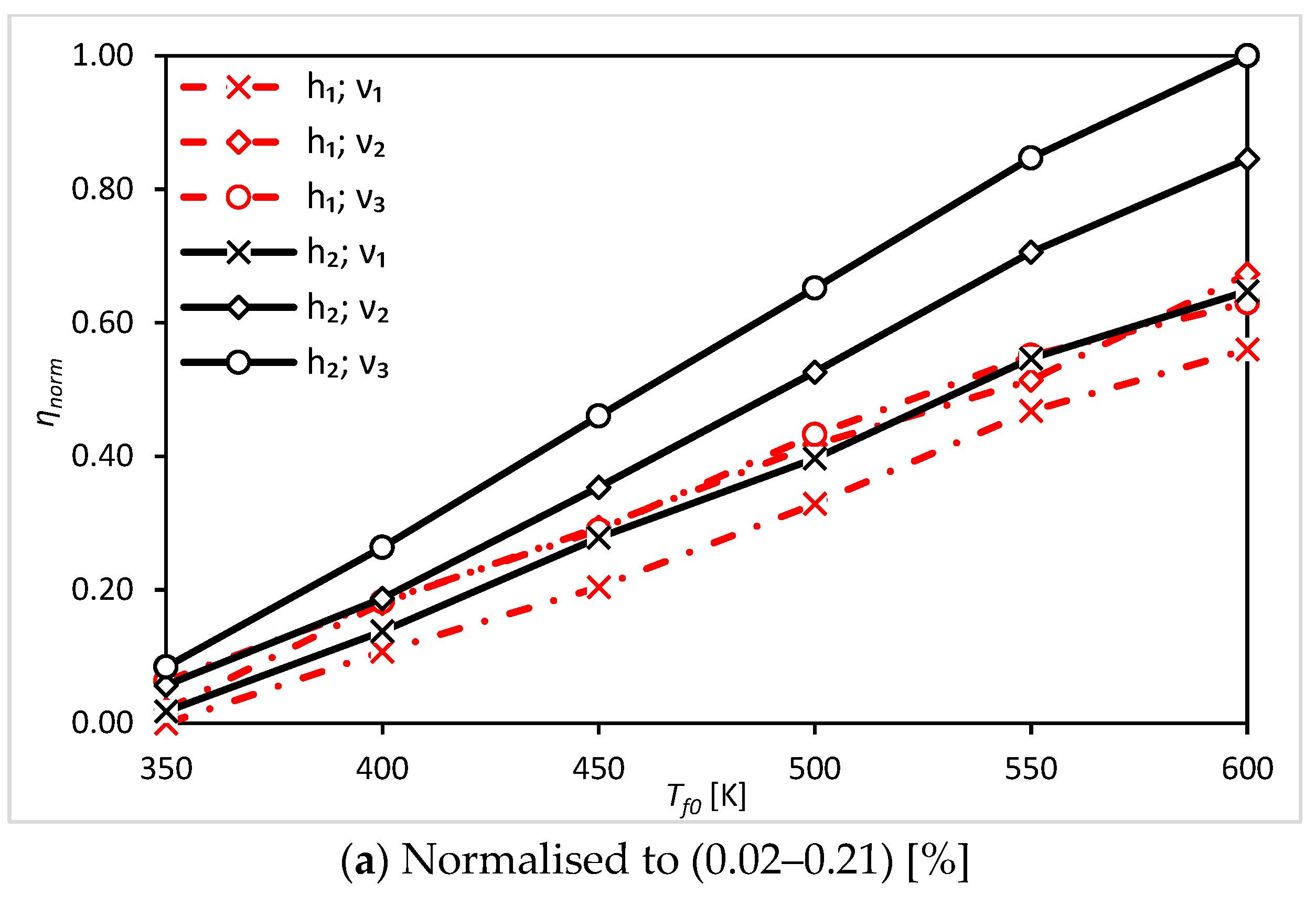
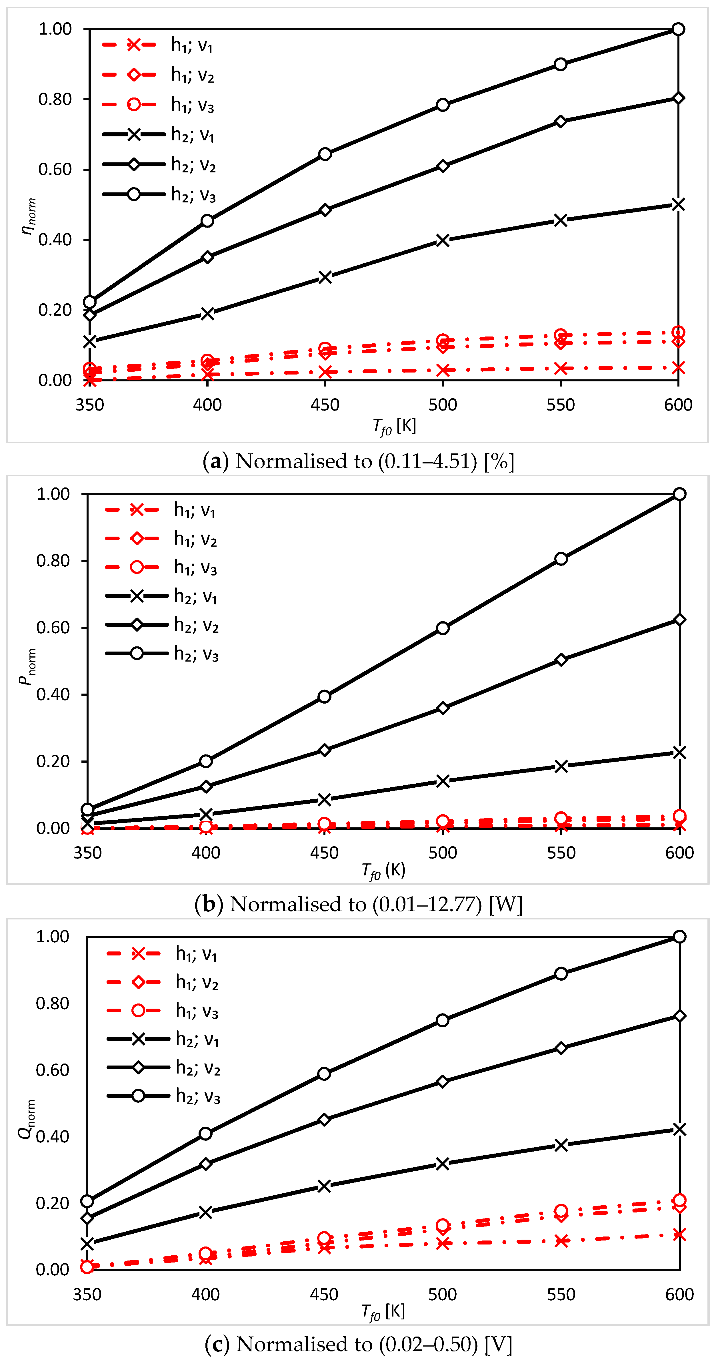
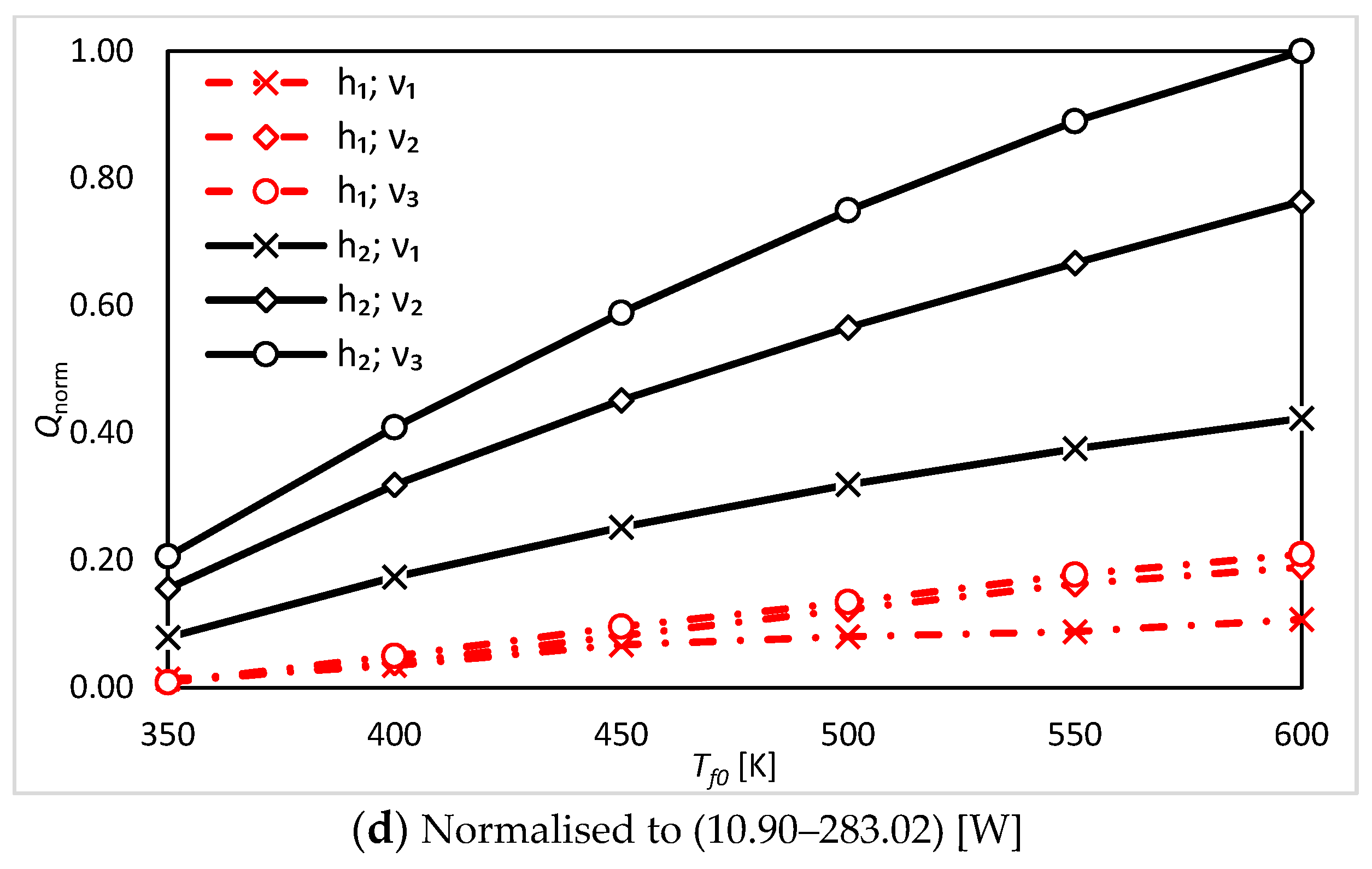
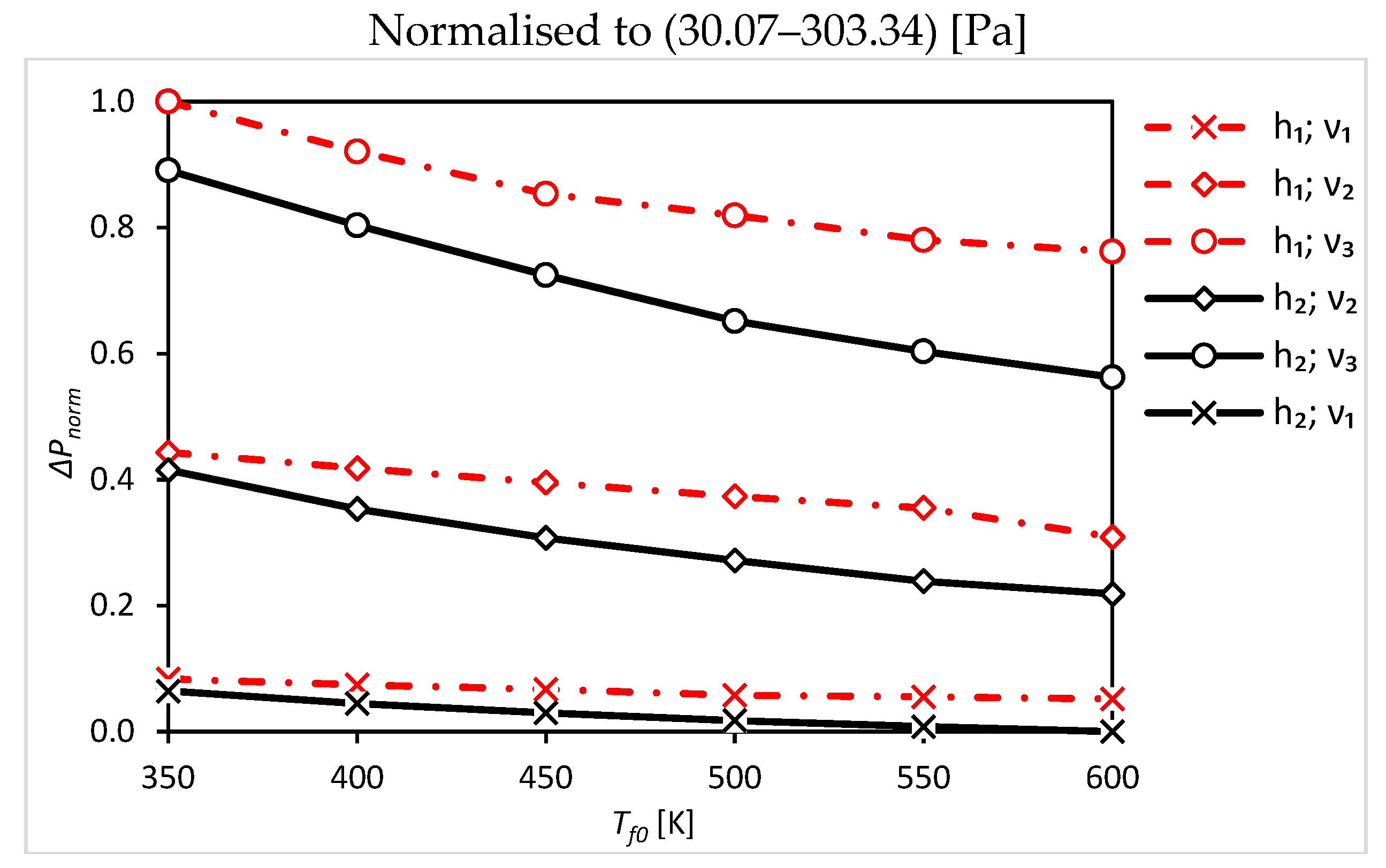
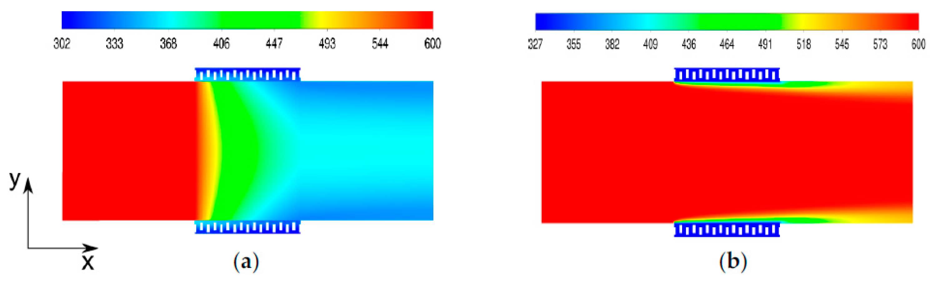
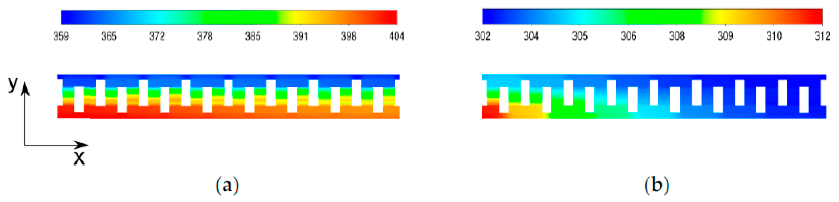
3. Results and Discussion

In order to evaluate the convergence of the simulations, residuals of the order of 10⁻³ for the continuity equation and 10⁻⁶ for the rest of the transport equations were established in order to guarantee a good accuracy/computational time ratio. It was also necessary to define monitors, which allow verifying that the steady state has been reached in the system. These monitors are the electric current computed from Equation (19) and the temperature at the duct outlet. In addition, the values of efficiency, electrical power, potential difference and heat transferred in the central region were normalised as follows:

$${\eta }_{norm}=\frac{\eta -{\eta }_{min}}{{\eta }_{max}-{\eta }_{min}}$$

(27)

$$P_{norm}=\frac{P-P_{min}}{P_{max}-P_{min}}$$

(28)

$$\Delta {\psi }_{norm}=\frac{\Delta \psi -\Delta {\psi }_{min}}{\Delta {\psi }_{max}-\Delta {\psi }_{min}}$$

(29)

$$Q_{norm}=\frac{Q-Q_{min}}{Q_{max}-Q_{min}}$$

(30)

where the subscripts min and max represent the maximum and minimum values obtained in the simulations, respectively.

From the results shown in Figure 5a,b, it is observed that the simulations yielded conversion efficiencies and power outputs in the range of [0.016–0.21] [%] and [4.24 × 10⁻⁴–5.9 × 10⁻²] [W], respectively, both parameters being favoured by higher gas inlet velocities and temperature, as well as higher external heat dissipation coefficients. The low efficiencies achieved suggest, preliminarily, that such a system is not feasible for waste heat recovery under the operating and design conditions studied. Furthermore, from Figure 5c, values of potential difference between the ends of the thermoelectric device in the range of [2.44 × 10⁻³–3.21 × 10⁻²] [V] were obtained, showing an approximately linear trend for this variable, as well as its increase with increasing temperature and gas velocity. Finally, Figure 5d shows the heat transferred in the central region, which is in the range of [2.71–28.13] [W].

The recovery efficiency and power output values for the porous media system shown in Figure 6a,b are in the ranges [0.11–0.71] [%] and [0.012–0.481] [W], respectively, for the heat dissipation condition (h₁), while for the higher external heat dissipation coefficient (h₂), they are in the ranges [0.59–4.51] [%] and [0.19–12.77] [W], respectively. This is evidence of the great importance of the cold-side heat dissipation condition on the performance of the thermoelectric device, as a higher value of this parameter reduces the existing convective heat transfer resistance between the surrounding fluid and the top plate of the thermoelectric device, thus allowing the generation of a higher temperature gradient between the thermoelements. As a result, a more detailed study of the fluid flow through the cold side of the device is of great interest to establish optimal operational conditions for the system.

Likewise, an increase in the efficiency and power output of the device is observed as the thermal load of the fluid increases, which is consistent with the physics of the problem, as an increase in the inlet temperature produces a greater thermal gradient throughout the system. This favours heat transfer in the central region in accordance with Fourier’s law; thus, the energy flow allows a greater temperature difference to exist between the ends of the thermocouple, which in turns favours the development of a high electric flux through the Seebeck effect.

Although the efficiency of the device improves with an increase in the gas inlet temperature, the relationship is not linear but rather has a certain degree of concavity. This tendency is largely explained by the behaviour of the heat transfer shown in Figure 6d, as the rate at which heat is transferred to the thermocouple is lower than the rate at which the thermal energy of the gas stream increases, generating the characteristic shapes of these curves. With respect to the fluid inlet velocity, its increase improves the performance of the thermoelectric device due to the higher values of the interfacial heat transfer coefficient computed from Equation (8a), which, in addition, translates into an improvement in the heat transfer from the duct to the thermocouples.

Regarding the electric potential difference generated between the ends of the thermoelectric module shown in Figure 6c, values in the range of [0.019–0.0925] [V] and [0.048–0.5] [V] were obtained for the external heat dissipation coefficients h₁ and h₂, respectively. An approximately linear behaviour with respect to the gas inlet temperature is observed. It is observed that higher velocities generated higher potential differences in the thermoelectric device. Finally, Figure 6d shows the heat transferred in the central region, which is in the range of [10.9–283.02] [W].

Figure 7 shows the system pressure drops, which are in the range of [44.30–303.34] [Pa] and [30.07–273.53] [Pa] for the external heat dissipation coefficients h₁ and h₂, respectively. It can be seen that these are favoured by higher inlet velocities, as well as higher external heat dissipation coefficients and temperatures. Therefore, the effect of the latter factors on the fluid pressure drops shows how heat transfer induces a disturbance in the flow field.

In relation to the temperature contours shown in Figure 8a,b, it can be observed that the fluid temperature difference between the inlet and outlet of the duct is higher for the case with porous media, which shows significant improvements in the percentage of thermal energy recovered and justifies the results presented in Figure 5 and Figure 6.

With respect to the temperature contours of the thermoelectric device shown in Figure 9a,b, the temperature gradient formed in the thermoelectric devices for the duct with porous media is of greater magnitude, which explains its higher power outputs. It is also important to note that the free current temperature of the waste heat source and the surrounding media differs from that present at the ends of the thermoelectric device, due to the existence of boundary layers, which is why a fluid dynamic analysis is necessary to predict the behaviour of a system with these characteristics.

Figure 10a,b shows the voltage contours developed in the thermoelectric devices, showing a higher heat flow towards the thermocouples, which favours a higher movement of charge carriers in the thermocouples.

In relation to the pressure contours presented in Figure 11a,b, it is observed that there is no significant pressure variation in the clear fluid regions; pressure gradients are only found in the central region of the duct where the porous media are located.

From the velocity contours shown in Figure 12a,b, for the case with porous media, there is a perturbation of the flow field due to heat transfer because as the gas temperature decreases rapidly in the central region, an increase in density takes place, which results in a reduction of the fluid velocity through the system to comply with the continuity equation. By contrast, in the case without the porous matrix, the velocity does not undergo significant changes due to the deficient heat transfer in the system.

4. Conclusions

A numerical study was carried out on the thermogeneration of electricity using waste heat, finding that the insertion of a porous medium generated a significant increase in the overall efficiency and electrical power output values of the thermoelectric device compared to the system without a porous matrix.

For the range of variables analysed, it was found that the efficiency and power output values were favoured by an increase in the fluid inlet temperature and velocity, as well as by higher heat extraction rates in the central region. It was also possible to appreciate the existence of a non-linear relationship between the thermal load of the waste heat carrier stream and the efficiency of the system.

More significant pressure drops were observed in the central region of the problem due to the presence of porous media, which were enhanced by higher inlet velocities and temperatures as well as higher heat extraction rates.

This work represents a contribution to the design of systems and methods to increase the recovery rate of waste heat carried by working fluids in the industrial sector, as well as to the use of green technologies to convert waste heat into electricity and to improve the thermal efficiency of processes. Future studies could consider the use of other porous materials as well as other fluids that carry waste energy, both gases and liquids.

References

1. World Energy Outlook 2019. Available online: https://iea.blob.core.windows.net/assets/98909c1b-aabc-4797-9926-35307b418cdb/WEO2019-free.pdf (accessed on 1 October 2021).
2. Johnson, I.; Choate, W.T.; Davidson, A. Waste Heat Recovery Technology and Opportunities in U.S. Industry; EERE: Washington, DC, USA, 2008; pp. 10–13. [Google Scholar] [CrossRef]
3. Johansson, M.; Söderström, M. Electricity generation from low temperature industrial excess heat an opportunity for the steel industry. Energy Effic. 2014, 7, 203–215. [Google Scholar] [CrossRef] [Green Version]
4. Zhang, H.; Wang, H.; Zhu, X.; Qiu, Y.J.; Li, K.; Chen, R.; Liao, Q. A review of waste heat recovery technologies towards molten slag in steel industry. Appl. Energy 2013, 112, 956–966. [Google Scholar] [CrossRef]
5. Miró, L.; Bruckner, S.; Cabeza, L. Mapping and discussing industrial waste heat (iwh) potentials for different countries. Renew. Sustain. Energy Rev. 2015, 51, 847–855. [Google Scholar] [CrossRef] [Green Version]
6. Papapetrou, M.; Kosmadakis, G.; Cipollina, A.; La Commare, U.; Micale, G. Estimation of the technically available resource in the EU per industrial sector, temperature level and country. Appl. Therm. Eng. 2018, 138, 207–216. [Google Scholar] [CrossRef]
7. Gou, X.; Xiao, H.; Yang, S. Modeling, experimental study and optimization on low-temperature waste heat thermoelectric generator system. Appl. Energy 2010, 87, 3131–3136. [Google Scholar] [CrossRef]
8. Ismail, B.I.; Ahmed, W.H. Thermoelectric power generation using waste heat energy as an alternative green technology. Recent Pat. Eng. 2009, 2, 27–28. [Google Scholar] [CrossRef]
9. Mamur, H.; Ahiska, R. A review: Thermoelectric generators in renewable energy. Int. J. Renew. Energy Res. 2014, 4, 128–136. [Google Scholar]
10. Niu, X.; Yu, J.; Wang, S. Experimental study on low-temperature waste heat thermoelectric generator. Power Sources 2009, 188, 621–626. [Google Scholar] [CrossRef]
11. Liu, C.; Chen, P.; Li, K. A 1 KW thermoelectric generator for low-temperature geothermal resources. Trans.-Geotherm. Resour. Counc. 2014, 38, 749–754. [Google Scholar]
12. Arsie, I.; Cricchio, A.; Pianese, C.; Ricciardi, V.; De Cesare, M. Modeling analysis of waste heat recovery via thermo-electric generator and electric turbo-compound for co2 reduction in automotive si engines. Energy Procedia 2015, 82, 81–88. [Google Scholar] [CrossRef] [Green Version]
13. Crane, D.; Jackson, G. Optimization of cross flow heat exchangers for thermoelectric waste heat recovery. Energy Convers. Manag. 2004, 45, 1565–1582. [Google Scholar] [CrossRef]
14. Hendrick, T.; Choate, W. Engineering Scoping Study of Thermoelectric Generator Systems for Industrial Waste Heat Recovery; EERE: Washington, DC, USA, 2006; pp. 4–22. [Google Scholar] [CrossRef] [Green Version]
15. Gao, W.; Hodgson; Kong, L. Numerical analysis of heat transfer and the optimization of regenerators. Numer. Heat Transf. A 2006, 50, 63–65. [Google Scholar] [CrossRef]
16. Amiri, L.; Ghoreshi Madiseh, S.A.; Ferri, H.; Sasmit, A.P. A porous media based heat transfer and fluid flow model for thermal energy storage in packed rock bed. In Proceedings of the International Conference on Sustainable Energy and Green Technology, Kuala Lumpur, Malaysia, 20–22 August 2019; Volume 268. [Google Scholar] [CrossRef]
17. Pavel, B.I.; Mohamad, A.A. An experimental and numerical study on heat transfer enhancement for gas heat exchangers fitted with porous media. Int. J. Heat Mass. Transf. 2004, 47, 4439–4952. [Google Scholar] [CrossRef]
18. Hsu, C.; Huang, G.; Chu, H.; Yu, B.; Yao, D. Experiments and simulations on low-temperature waste heat harvesting system by thermoelectric power generators. Appl. Energy 2011, 88, 1291–1297. [Google Scholar] [CrossRef]
19. Rowe, D. Thermoelectric waste heat recovery as a renewable energy source. Int. J. Innov. Energy Syst. Power 2006, 1, 13–23. [Google Scholar]
20. Tang, Z.; Deng, Y.; Su, C.; Shuai, W.; Xie, C. A research on thermoelectric generator’s electrical performance under temperature mismatch conditions for automotive waste heat recovery system. Case Stud. Therm. Eng. 2015, 5, 143–150. [Google Scholar] [CrossRef] [Green Version]
21. Orr, B.; Akbarzadeh, A.; Mochizuki, M.; Singh, R. A review of car waste heat recovery systems utilizing thermoelectric generators and heat pipes. Appl. Therm. Eng. 2016, 101, 490495. [Google Scholar] [CrossRef]
22. Uyanık, T.; Ejder, E.; Arslanoğlu, Y.; Yalman, Y.; Terriche, Y.; Su, C.-L.; Guerrero, J.M. Thermoelectric Generators as an Alternative Energy Source in Shipboard Microgrids. Energies 2022, 15, 4248. [Google Scholar] [CrossRef]
23. Donoso-García, P.; Henríquez-Vargas, L. Numerical study of a waste heat recovery thermogenerator system. J. Braz. Soc. Mech. Sci. Eng. 2019, 41, 356–364. [Google Scholar] [CrossRef]
24. Henríquez-Vargas, L.; Donoso-García, P. Numerical study of thermoelectric generation within a reciprocal flow porous media burner. J. Mech. Eng. Autom. 2013, 3, 367–377. [Google Scholar]
25. Henríquez-Vargas, L.; Loyola, J.; Sanhueza, D.; Donoso-García, P. Numerical Study of Reciprocal Flow Porous Media Burners Coupled with Thermoelectric Generation. J. Porous Media 2015, 18, 257–267. [Google Scholar] [CrossRef]
26. Henríquez-Vargas, L.; Maiza, M.; Donoso-García, P. Numerical study of thermoelectric generation within a continuous flow porous media burner. J. Porous Media 2013, 16, 933–944. [Google Scholar] [CrossRef]
27. Donoso-García, P.; Henríquez-Vargas, L. Numerical study of turbulent porous media combustion coupled with thermoelectric generation in a recuperative reactor. Energy 2015, 93, 1189–1198. [Google Scholar] [CrossRef]
28. Nesarajah, M.; Frey, G. Thermoelectric power generation: Peltier element versus thermoelectric generator. In Proceedings of the IECON Proceedings, Florence, Italy, 24–27 October 2016. [Google Scholar] [CrossRef]
29. Hebei, L.T. TEC1-12706 Data Sheet. Available online: https://peltiermodules.com/peltier.datasheet/TEC1-12706.pdf (accessed on 12 August 2021).
30. ANSYS Fluent Theory Guide; Release 18.0; ANSYS Inc.: Canonsburg, PA, USA, 2018.
31. Dobrego, K.; Gnesdilov, N.; Kozlov, I.; Bubnovich, V.; Gonzalez, H. Numerical investigation of the new regenerator-recuperator scheme of VOC oxidizer. Int. J. Heat Mass. Transf. 2005, 48, 4695–4703. [Google Scholar] [CrossRef]
32. Gnesdilov, N.; Dobrego, K.; Kozlov, I. Parametric study of recuperative VOC oxidation reactor with porous media. Int. J. Heat Mass. Transf. 2007, 50, 2787–2794. [Google Scholar] [CrossRef]
33. Kaviany, M. Principles of Heat Transfer in Porous Media, 2nd ed.; Ling, F., Ed.; Springer: New York, NY, USA, 1991; pp. 368–369. [Google Scholar]
34. Henríquez-Vargas, L.; Bubnovich, V.; Donoso-García, P.; Cubillos, F. Modeling, simulation, and control for a continuous flow porous media burner. J. Porous Media 2013, 16, 155–165. [Google Scholar] [CrossRef]
35. Antononova, E.E.; Looman, D.C. Finite elements for thermoelectric device analysis in ANSYS. In Proceedings of the International Conference on Thermoelectrics ICT, Clemson, SC, USA, 19–23 June 2005. [Google Scholar] [CrossRef]
36. Donoso-García, P. Study of the Thermogeneration of Electricity by Combustion in Inert Porous Media under a Turbulent Fluid Dynamic Regime in a Recuperative Reactor. Ph.D. Thesis, Universidad de Santiago de Chile, Santiago, Chile, 2011. [Google Scholar]
37. Henríquez, J. Numerical Modeling and Simulation in Waste Heat Recovery Processes through Porous Media. Undergraduate Thesis, Universidad de Santiago de Chile, Santiago, Chile, 2020. [Google Scholar]
38. Patankar, S. Numerical Heat Transfer and Fluid Flow, 1st ed.; Minkowycz, W., Sparrow, E., Eds.; Hemisphere Publishing Corporation: Philadelphia, PA, USA, 1980. [Google Scholar]
39. Jaegle, M. Multiphysics Simulation of Thermoelectric Systems-Modeling of Peltier-Cooling and Thermoelectric Generation. In Proceedings of the COMSOL Conference 2008, Hannover, Germany, 4–6 November 2008. [Google Scholar]
Figure 1. Schematic of the waste heat recovery system based on thermogeneration of electricity.
Energies 15 05597 g001
Figure 2. Schematic of a conventional thermoelectric module.
Energies 15 05597 g002
Figure 3. Schematic of the N n thermocouples connected electrically in series [36].
Energies 15 05597 g003
Figure 4. Axial velocity profiles for different mesh sizes.
Energies 15 05597 g004
Figure 5. Results of simulations without porous matrix: (a) Overall efficiency; (b) Electrical power; (c) Electric potential; (d) Heat transferred in the duct.
Energies 15 05597 g005aEnergies 15 05597 g005b
Figure 6. Results of simulations with porous matrix: (a) Overall efficiency; (b) Electric power; (c) Electric potential; (d) Heat transferred in the duct.
Energies 15 05597 g006aEnergies 15 05597 g006b
Figure 7. Pressure drops of the system with porous media.
Energies 15 05597 g007
Figure 8. Temperature contours of the system [K]: (a) with porous media; (b) without porous media.
Energies 15 05597 g008
Figure 9. Temperature contours of the thermoelectric device [K]: (a) with porous media; (b) without porous media.
Energies 15 05597 g009
Figure 10. Voltage contours [V]: (a) with porous media; (b) without porous media.
Energies 15 05597 g010
Figure 11. Pressure contours [Pa]: (a) with porous media; (b) without porous media.
Energies 15 05597 g011
Figure 12. Darcy velocity contours [m·s−1]: (a) with porous media; (b) without porous media.
Energies 15 05597 g012