A Forecasting Model of Wind Power Based on IPSO–LSTM and Classified Fusion

Abstract

To improve the predicting accuracy of wind power, this paper proposes a forecasting model of wind power based on the IPSO–LSTM model and classified fusion, which not only overcomes the shortcoming of the artificially determined parameters of LSTM, but also solves the problem that the fused accuracy may be reduced by the environment when adopting a single fusion model. Firstly, some wind speed sub-series were obtained by decomposing the original wind speed according to the wavelet packet decomposition (WPD), and the data sets formed by combining these sub-series with meteorological elements. Subsequently, the wind power components formed by wind speed decomposition are predicted through the long short-term memory neural network (LSTM), which is optimized by the improved particle swarm optimization (IPSO). Consequently, the predicting value of the final wind power was acquired by adopting the method of classified fusion to calculate the wind power components. Several case studies were carried out on the proposed model with the help of Python. It is found from those relevant results that the RMSE and MAE of the proposed model is 1.2382 and 0.8210, respectively. Moreover, the R² is 0.9952. Those simulating results show that the proposed model may be better for fitting the actual curve of wind power and has excellent predicting accuracy.

1. Introduction

As a clean and renewable resource, wind energy has been paid more and more attention, which developed rapidly all over the world [1,2,3,4,5]. Due to the rising scale of grid-connected wind power, the intermittency, volatility, and uncertainty of wind energy bring great challenges to the planning and dispatching of a power system [6,7,8,9,10,11]. However, the short-term forecast of wind power can provide basic information for dispatchers. Therefore, during the process of power planning and dispatching, there is an urgent need to make accurate short-term forecasts of wind power in advance for a period of time in the future, in order to enhance the safety, stability, and economy of the power network.

Neural networks are widely used in the forecasting field of wind power, due to their adaptive and good non-linear mapping ability [12,13,14,15,16]. In particular, recurrent neural networks (RNN), with the capability of maintaining states between different inputs, show an advantage in handling time sequences, but there are some disadvantages such as vanishing and exploding gradients. LSTM, as an extension of the RNN, may deal with the problem of vanishing gradients by introducing memory cells with controlling gates, and are used extensively to simulate the time-series correlation [17]. Nevertheless, it is difficult to determine the number of neurons, the learning rate, and the iteration times of the LSTM, which may have a great influence on the generalized ability, the training time, and the predicting accuracy. For example, a forecasting model of wind power based on the RNN of the LSTM was proposed in [18], which can implement a more accurate forecast of wind power according to the characteristic of the sequence dependence characteristic of the RNN by training with the smaller data sets. A hybrid model of the VMD–Kmeans–LSTM was proposed in [19], which is applied to short-term prediction of wind power with multiple scales. The advantage of the proposed model is the ability to fit on multiple scales. A short-term forecasting model of wind power including the variational mode decomposition (VMD), the convolutional LSTM (ConvLSTM) predictor, and error series modelling was proposed in [20], which can significantly increase the predicting accuracy. However, the initial parameters of the LSTM network of models mentioned above are determined by experiments, which result in a large computational cost in obtaining the optimal parameters, and may affect the predicting accuracy to a certain extent. Therefore, the introduction of an optimization algorithm can overcome the shortcoming of the artificially determined parameters of LSTM and automatically find the parameters, thus, improving the predicting accuracy. In addition, considering the high autocorrelation and the inherent volatility of the wind speed, there are large errors in directly predicting the wind power with the original time-series of wind speed, which may affect the predicting accuracy of wind power. A forecasting model of wind speed based on the WPD and artificial neural networks was established in [21], which decomposed the original series of wind speed, and employed the back-propagation neural network optimized by the criss-cross optimization algorithm to predict the wind speed with components of different frequency bands after decomposition, and the results show that the proposed method has the minimum absolute error. The unstable time-series of wind and solar power are decomposed into smooth subsequences by VMD [22,23,24], which reduces the undesirable effects caused by the volatility of the original series. With the help of the adaptive multiscale mathematical morphological algorithm, the original sequence of wind speed is decomposed into a series of subsequences, with different frequencies and fluctuant levels in the time domain [25]. Wavelet velocity is used to decompose the wind speed in [26], and neural networks with different structures are used to discover the regularity of the wind power in different frequency bands. In the literature mentioned above, the methods of comprehensive calculation of proposed models for the predicted component of wind power are relatively simple. However, the performance of each predicting model changes with the surrounding environment of the wind turbines, which may result in the different mapping relationship between predicting results and actual wind power. If a method of simple comprehensive calculation was employed to calculate the wind power at each moment only, the predicting accuracy would be significantly affected. Therefore, a method of classified fusion can fuse the components of wind power. In addition, to solve the problem that a single algorithm cannot adapt to the forecasting scenarios of different months in the whole year, an ultra-short-term wind power forecasting model was established in [27], which combines four different models of machine learning to predict wind power with a single model, and the final forecasting results are obtained by the data fusion performed on the forecasting results in the same period. Compared with a single model of prediction, the ensemble method of prediction would be applied to different weather conditions, which can improve the predicting accuracy of wind power. Nevertheless, the forecasting effect of wind power is very poor when the correlation between meteorological factors and the wind power is predicted to be strong, and adding the Numerical Weather Prediction (NWP) to the combined forecasting method should be considered. The NWP data are the numerical meteorological information obtained from meteorological centers or local meteorological forecasts of wind farms.

Therefore, for enhancing the predicting accuracy of wind power, the objective of this paper is to propose a forecasting model of wind power based on IPSO–LSTM and classified fusion. The contributions of this paper are (1) for the sake of overcoming the shortcoming of the artificially determined parameters of LSTM, the LSTM optimized by IPSO was employed to predict the components of wind power. (2) Consider the variability of the environment surrounding wind turbines, which may cause the change in the performance of each predicting model accordingly. As the mapping relationship between different predicting results and actual wind power will be different, a method of classified fusion was adopted to fuse these components in this paper. (3) A mutual iteration optimization framework of the classification model of the fusion pattern and fusion model is employed to obtain the optimal classification model of the fusion pattern and the corresponding fusion model.

2. Overall Framework of the Forecasting Model of Wind Power

A forecasting model of wind power based on IPSO–LSTM and classified fusion is proposed in this paper; the overall framework of the proposed model is shown in Figure 1.

The steps to establish the forecasting model of wind power in this paper are as follows:

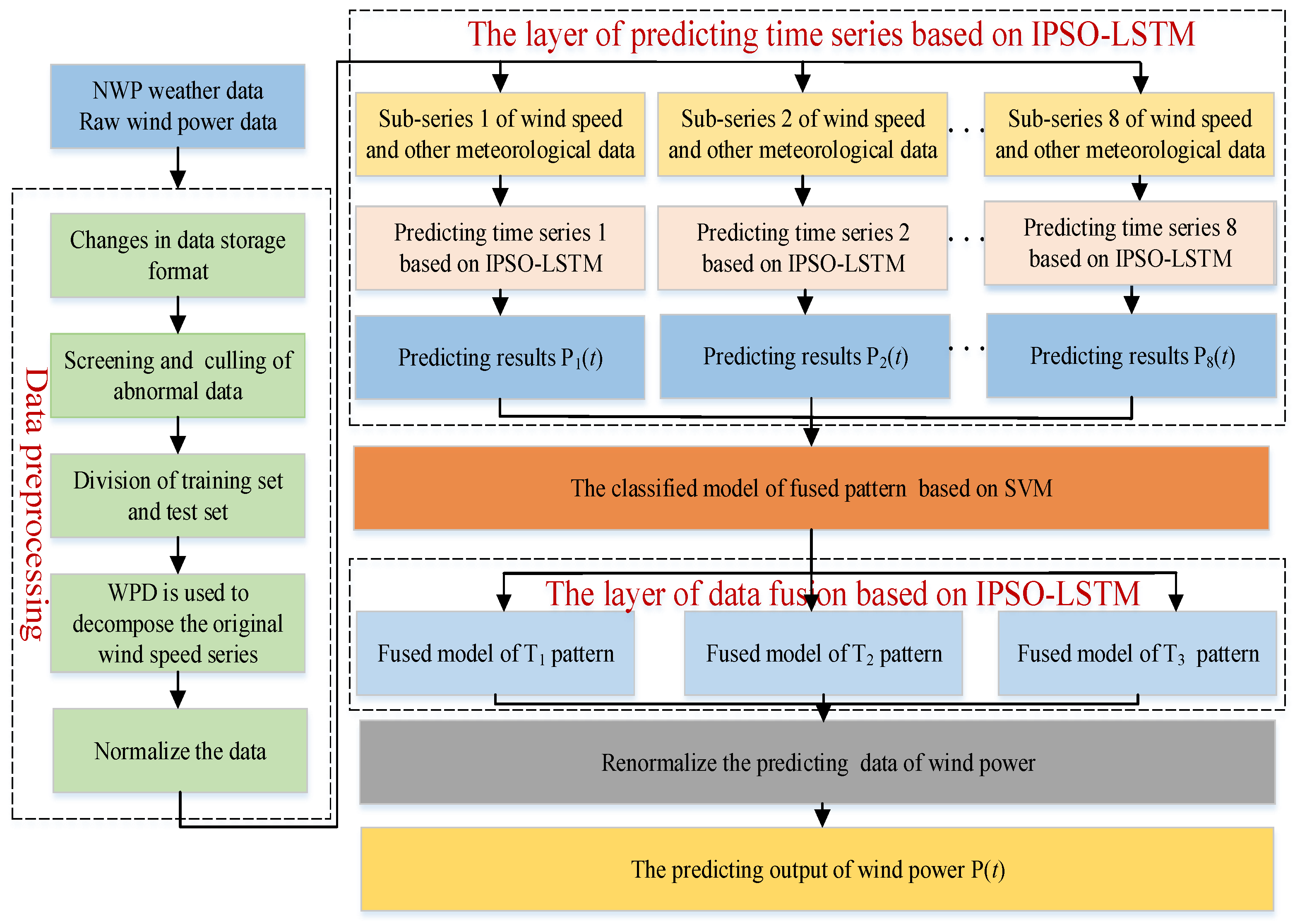
(1)

In the pre-processing phase of the data, a three-level decomposition for the original time-series of wind speed is performed with the help of the WPD, and the eight sub-sequences of wind speed for different frequency bands are acquired;

(2)

There are eight predicting models on basis of the IPSO–LSTM that can be established in accordance with the eight sub-sequences of wind speed in step (1). The input of the predicting model is the sequence of wind speed for each frequency band and other meteorological data, and the output is the predicted value of wind power for eight sub-sequences;

(3)

The classification model of fusion pattern optimized by the framework of iterative optimization is used to select a fusion mode for the power time-series of each time period;

(4)

The fusion mode corresponding to step (3) is selected, and multiple predicted values of wind power in each period time are fused into one value, which is the final predicted value of wind power.

3. The Construction of the Forecasting Model Based on the IPSO–LSTM and Classified Fusion

3.1. The Pre-Processing of the Data

3.1.1. Normalization

The data sets used in the case study include wind power, wind speed, ambient temperature, relative humidity, and component temperature. Due to the different scales and dimensions of each data set, the z-score method was adopted in this paper to standardize the data, in order to achieve the best performance of the model. Assuming that the data used this time are $X=\left(x_1,x_2,\cdots ,x_j,\cdots ,x_i\right)$, there are $n$ samples $x_j=\left(x_j^1,x_j^2,\cdots ,x_j^t,\cdots ,x_j^n\right)$ for each feature $x_j$, and then the z-score standardization formula is:

$$x_j^{t\prime }=\frac{x_j^t-{\mu }_j}{\sqrt{\frac{1}{N}{\displaystyle \sum _{t=1}^N{\left(x_j^t-{\mu }_j\right)}^2}}}$$

(1)

where ${\mu }_j$ represents the average value of features $x_j$, $N$ represents total number of samples, and $x_j^t{}^{\prime }$ represents standardized data.

Using standardized data as the input of the model can reduce the influence of different dimensions of characteristic parameters on the performance of the model, and improve the predicting accuracy and generalization ability of the model.

3.1.2. The Pre-Processing of the Data Based on WPD

Due to the characteristics of the wind speed of high autocorrelation and inherent volatility, there are large errors in directly predicting the wind power with the original time-series of wind speed, which may affect the predicting accuracy of wind power. Therefore, for further enhancement of the predicting accuracy of wind power, this paper performs a multi-scale decomposition of the original series of wind speed in the pre-processing phase of the data, with the help of the WPD. The WPD is generated and is developed on the basis of wavelet transformation, which can help grasp the detailed characteristics of the signals, and improve the temporal resolution of the signals; it is widely applied to deal with complex slowly changed signals [28].

A three-level decomposition for the original time-series of wind speed was conducted with the help of the WPD in this paper. The reconstructed signals of each node are demonstrated in Figure 2.

3.2. Construction of Predicting Model Based on IPSO–LSTM

Due to the sequence of wind speed being decomposed into multiple stationary components in the preprocessing stage of the data, it is necessary to establish multiple sub-models to predict the wind power of different frequency bands. The inputs of each sub-model are the decomposed sub-series of wind speed, other meteorological elements (ambient temperature, relative humidity, and atmospheric pressure), and component temperature. The LSTM has excellent predicting accuracy in the prediction of wind power [29]. However, it is difficult to determine the number of neurons, the learning rate, and the iteration times of the LSTM, which may impact the generalized ability, training time, and predicting accuracy of the model greatly. Therefore, this paper improves the PSO (IPSO) to enhance the optimization ability of the algorithm, and uses the IPSO to optimize parameters of LSTM, such as the learning rate, the number of iterations, and the number of hidden layer neuron nodes. The flow chart is shown in Figure 3.

3.2.1. The IPSO Algorithm

The PSO has the risk of falling into a locally optimal solution. Therefore, when using the PSO to optimize the LSTM, it is necessary to improve the PSO for obtaining better parameters to optimize the LSTM in the practical application. The Algorithm 1 can be improved as follows:

Algorithm 1: IPSO

1:      Do

2:           For each particle

3:                Calculate its fitness value;

4:           If (The fitness value Xi of is better than the historical best value Pi of the particle)

5:                Update historical best individual Pi with Xi:

6:           End

7:           Select the best particle in the current particle swarm

8:           If (The current best particle is better than the historical best particle of the swarm)

9:                Update the best particle of the swarm Pg with current swarm best particle

10:           For each particle

11:                Update the weight w according to Formula (2);

12:                Update particle velocity;

13:                Update particle position;

14:                Adaptive mutation according to Formula (3);

15:           End

16: While the maximum number of iterations or the minimum error has not been reached

(1) The fixed inertia weight w in the PSO weakens the ability of global optimization and the convergent speed of the algorithm; there are some scholars who introduce the coefficient of inertia weight in the PSO to realize the effective control of the velocity of the particle. In this article, the w can be improved to enhance the performance of the PSO, as shown in (2).

$$w=w_{\max }-\frac{(w_{max}-w_{min})}{(1+e^{-t/t_{max}})}$$

(2)

where w_max and w_min stand for the maximum and minimum values of w, respectively. t stands for the number of the current iteration, and t_max stands for the maximum number of the iteration. It can be seen from Equation (2) that the w gradually decreases with the t gradually increasing, which indicates the former weight is significant and the latter weight is small. In this way, the update speed is accelerated and the globally optimized ability improved when the globally optimal solution is not found in the early stage of optimization. In the later stage, the update speed may be slowed down, and the locally optimized ability may be enhanced, when the globally optimal solution is near.

(2) The mutation operation in the genetic algorithm can be added to the PSO for adaptive mutation. Its probability of variation can be expressed as (3).

$$rand>0.5\times \frac{t}{t_{\max }}+0.5$$

(3)

where t represents the number of the current iteration, t_max stands for the maximum number of iterations, and rand represents a random number in the range [0, 1]. As can be easily observed from (3), the right side of the inequality gradually increases from 0.5 to 1 with the increase in the evolutionary algebra. As the right side of the inequality gradually increases, the probability of the inequality being established gradually decreases, which leads to the probability of the particle mutating decreasing, and, thus, the risk of the particle falling into a locally optimal solution is reduced.

In order to verify the ability of optimization for the IPSO, the IPSO and the PSO can be used to search for the extreme value of a five-dimensional sphere function (the extreme value is 0). For a more intuitive observation, the logarithms are taken for the results of the optimization in the paper, as displayed in Figure 4.

Figure 4 manifests that the PSO falls into the locally optimal solution with an optimal result about of 1.2 when it iterates about 40 times. However, the IPSO still has the optimized ability when iterating 1000 times, and its optimal result at this time is about 10⁻⁷. Comparing the optimal result of the IPSO with that of the PSO, the IPSO is about six orders of magnitude different from that of the PSO, which verifies that the IPSO significantly enhances the optimized ability.

3.2.2. The IPSO–LSTM Algorithm

(1)

Long short-term memory neural network

The LSTM makes the memory information in a time-series controllable by adding memory units to each natural unit of the hidden layer, on the basis of the RNN. The memory and forgetting degree of the previous information and the current information can be controlled through several controllable gates (input gate, forgetting gate, and output gate) during the transmission between each unit of the hidden layer. Thus, the RNN network has the function of long-term memory, which can effectively avoid the problem of gradient disappearance; the structure of LSTM is demonstrated in Figure 5.

The update formulas of the three control gates and unit information are as follows:

The forget gate f(t) sets the weight of the elements in the state c_t−1 of the previous moment through the current input x_t and the output h_t−1 of the previous moment. The ranges of weight value from 0 to 1, as shown in (4):

$$f_t=\sigma (W_f\left[h_{t-1};x_t\right]+b_f)$$

(4)

The update of the new state is completed by the input gate i(t). The input gate determines which parts of the c_t−1 state are written into the current state c_t according to x_t and h_t−1, as shown in (5):

$$i_t=\sigma (W_i\left[h_{t-1};x_t\right]+b_i)$$

(5)

Meanwhile, the candidate value ${\tilde{c}}_t$ of the new state is generated by tanh function, and the formula for calculating ${\tilde{c}}_t$ is as follows:

$${\tilde{c}}_t=\tanh (W_{\tilde{c}}\left[h_{t-1};x_t\right]+b_{\tilde{c}})$$

(6)

The new state c_t is jointly determined by f(t), i(t), ${\tilde{c}}_t$ and c_t−1, as shown in (7):

$$c_t=f_t\otimes c_{t-1}+i_t\otimes {\tilde{c}}_t$$

(7)

Similarly, output gate o_t is expressed as (8):

$$o_t=\sigma (W_o\left[h_{t-1};x_t\right]+b_o)$$

(8)

The final h_t of LSTM is determined by output gate o_t and c_t, as shown in (9):

$$h_t=o_t\otimes \tanh (c_t)$$

(9)

In (4)~(9), W denotes the weight matrix, b denotes the bias terms. ⊗ denotes the element-wise multiplication.

(2)

The LSTM optimized by the IPSO

The predicting effect of the neural network can be directly reflected by the mean square error of test sets. In the existing studies, most fitness values only select the mean square error of training samples, and the predicting effect of the model loses its optimality when the fitting occurs. Therefore, the mean square error of the training set and the test set is expressed as the fitness function in this paper, and the weight of both is 0.5. The fitness function of this model is calculated through adding the mean square error of the training set and the test set, then multiplying the weight, as demonstrated in (10):

$$fi{t}_i=0.5\times {\displaystyle \sum _{j=1}^J\frac{{\widehat{y}}_t^j-y{}_t{}^j}{y_t^{\mathrm{j}}}}\times 100+0.5\times {\displaystyle \sum _{k=1}^K\frac{{\widehat{y}}_y^k-y{}_y{}^k}{y_y^{\mathrm{k}}}}\times 100$$

(10)

where ${\widehat{y}}_t^j$ denotes the output value of the training set, and ${\widehat{y}}_y^k$ denotes the output value of the test set. $y_t^j$ and $y_y^k$ denote the desired output of the training set and the test set, respectively. The flow of the IPSO–LSTM algorithm is illustrated in Figure 6.

3.3. Construction of the Classification Model of Fusion Pattern Based on SVM and Fusion Model

The performance of each predicting model changes with the environment surrounding wind turbines, which results in a different mapping relationship between different predicting results and actual wind power. If a single fusion model was used to fuse the wind power at each moment only, the fused accuracy would be significantly affected. Therefore, a classified method of fusion pattern is proposed to fuse the components of wind power in this paper, which is composed of the optimal classification model of fusion pattern and the corresponding fusion model. Moreover, the LSTM is a mature machine algorithm, and the IPSO–LSTM is optimized on the basis of the LSTM, which can adapt to different requirements of application. Therefore, the IPSO–LSTM is still applied to establish the model of data fusion in this paper. The flow chart is exhibited in Figure 7.

The SVM adopts a learning method of structural risk minimization, which can effectively avoid overfitting and local optimization in the learning environment of small samples [30]. Therefore, in this paper, the SVM is employed to establish a classification model of fusion pattern; the principle of the SVM is a method of binary classification based on statistical theory. The given training samples can be expressed as (11):

$$D=\{(x_i,y_i),i=1,2,\dots ,l\},x_i\in R^d$$

(11)

where $x_i\in R^d$ represents the input variable, and $y_i\in R$ represents the corresponding output value. The most fundamental goal of SVM is to obtain a partition hyperplane (w, b), which classifies samples belonging to the same category into one side, and the samples belonging to other categories into other spaces. In the multi-dimensional space composed of training sample set D, the partition of hyperplane can be expressed by the following linear equation:

$$w{x}_i+b=0$$

(12)

where the vertical normal of the hyperplane is directly determined by $w^{{\rm T}}=(w_1,w_2,\dots w_d)$, and b denotes the displacement term, which represents the vertical distance between the partition hyperplane and the sample point.

When the structure and parameters of each model are determined, the forecasting values of wind power P₁(t)~P₈(t), based on the decomposed sequence of wind speed and other influencing factors in each time period by simulation, and the actual values of wind power P₀(t) in each time period can be acquired.

4. Algorithm of Mutual Iterative Optimization for Classified Fusion

In order to classify the fusion patterns and establish the corresponding fusion models automatically, an optimal framework with mutually iteration could be proposed, which uses the results of the classification model for the fusion pattern to train the fusion model. Furthermore, the classification model of the fusion pattern is updated according to the fused accuracy of the returned fusion model, which can form a calculating cycle. In the cycle, the two kinds of models can be modified and updated constantly until they cooperate perfectly, and the cycle ends when the data labels obtained according to the classification are consistent with the data labels according to the fused accuracy. The optimal framework of mutually iteration is exhibited in Figure 8 [26].

Figure 8 shows the process of the optimal framework of mutually iteration as follows:

(1)

Setting the value of k to 1, the predicting results of power for different frequency bands in each time period can be divided into n classes by the k-means algorithm, so as to obtain different labels of the fusion patterns;

(2)

The different labels of fusion modes obtained in step (1) are employed to train the different fusion models. All predicting results of power belonging to the fusion model can be taken as input, and the actual power can be taken as output;

(3)

The predicting results of all time periods are input into each fusion model. The fusion model that makes the fused results of each time period closest to the actual value is selected as the fusion pattern of this time period. The data is reclassified into different fusion patterns on the basis of the classified principle mentioned above;

(4)

The classification model may be trained with the classified results in step (3);

(5)

If the iteration continues, the classification model of the pattern can be used to reclassify the data of each time period and the value of k is increased by 1. In this way, the process will return to step (2) to continue to execute. If the iteration is terminated, the classification model of fusion pattern and its corresponding fusion model can be saved as the optimal model required by the study.

5. Case Studies

The proposed wind power prediction model is implemented in Python in PyCharm editor and MATLAB. Data preprocessing, such as wavelet packet decomposition, is performed in MATLAB, algorithms such as IPSO and SVM and parameter search for LSTM are implemented in Python, and the TensorFlow framework in Python is used to build LSTM models with different parameters to achieve accurate prediction of wind power.

This paper proposes a short-term predicting model of wind power based on IPSO–LSTM and classified fusion, the data set used in this case study is the measurement data of a wind farm in 2018, with a time resolution of 15 min. Some data sets of this experiment are listed in

Table 1. Partial data sets of this experiment.

Time	Wind Speed (m/s)	Component Temperature	Environment Temperature	Air Pressure (hpa)	Relative Humidity	Actual Generating Power (MW)
1 January 2018 07:45	4.94	4.27	1.53	992.02	50	4.34
1 January 2018 08:00	3.87	6.03	1.84	992.21	51	7.43
1 January 2018 08:15	4.02	9.05	1.94	992.50	51	10.47
1 January 2018 08:30	4.18	9.57	2.24	992.70	52	13.51
1 January 2018 08:45	4.02	10.72	2.45	992.60	53	23.44
1 January 2018 09:00	4.18	12.38	2.86	992.70	54	33.77
1 January 2018 09:15	2.95	11.55	2.96	992.50	55	39.07
1 January 2018 09:30	3.41	12.17	3.47	992.50	55	45.58
1 January 2018 09:45	4.18	13.94	4.08	992.50	54	51.23
1 January 2018 10:00	3.87	13.32	4.39	992.31	55	55.76
1 January 2018 10:15	3.72	14.98	4.59	992.31	53	62.37
1 January 2018 10:30	3.56	16.54	5.10	992.31	54	66.62
1 January 2018 10:45	2.19	16.65	5.31	992.31	56	69.27
1 January 2018 11:00	2.34	17.06	5.82	992.41	56	72.16
1 January 2018 11:15	3.72	18.31	6.22	992.41	57	75.25
1 January 2018 11:30	2.8	18.10	6.63	992.50	57	77.03
1 January 2018 11:45	0.22	19.56	6.94	992.70	57	78.63
1 January 2018 12:00	2.12	18.94	7.35	992.80	57	80.17
1 January 2018 12:15	1.73	19.66	7.55	992.80	57	79.74
1 January 2018 12:30	0.6	19.77	7.86	992.80	58	77.13
1 January 2018 12:45	0.38	18.62	8.06	992.70	58	44.52
1 January 2018 13:00	1.57	19.46	8.16	992.60	59	41.77
1 January 2018 13:15	2.49	17.79	8.57	992.60	60	34.20
1 January 2018 13:30	2.95	18.73	8.57	992.60	61	27.11
1 January 2018 13:45	2.19	16.65	9.08	992.60	57	31.16
1 January 2018 14:00	3.72	18.62	9.29	992.89	56	32.51

.

For the classification model of the fusion pattern and data fusion model, this paper selects 700 continuous time periods to test the model at different times. The first 600 data are used for model training, and the last 100 data are used to test the trained model.

Ι. For the sake of verifying that the decomposition of series for wind speed can reduce the influence for volatility and instability of wind speed on the prediction of wind power, in this paper the predicting value of wind power of the IPSO–LSTM without decomposing the wind speed is compared with the predicting value of the IPSO–LSTM with decomposing the wind speed. The results are displayed in Figure 9.

It is easily seen from Figure 9 that the trends of the predicting value of wind power based on the IPSO–LSTM are similar to the actual values of wind power when the wind speed is decomposed, which verifies the effectiveness of the proposed model. Moreover, the predicted value of the decomposed wind speed is more accurate than the non-decomposed one. As the wind speed has high autocorrelation and inherent volatility, this affects the predicting accuracy of wind power. Decomposing the wind speed into steadily multiple components, and predicting the components, separately, can greatly reduce the impact and improve the predicting accuracy.

In order to show the difference in performance and predicting accuracy of each model more clearly, there are three error indexes of root-mean-square error (RMSE), mean absolute error (MAE), and coefficient of determination (R²) that can be employed to evaluate the accuracy in this paper. The evaluation indexes of each model are listed in

Table 2. Evaluation indexes with and without decomposing wind speed.

Model	RMSE	MAE	R2
Decomposed wind speed	2.2842	1.4130	0.9838
Non-decomposed wind speed	6.8863	3.8607	0.8527

. For a more intuitive display, each evaluation index is displayed with a bar chart, as illustrated in Figure 10.

Furthermore, it is clearly observed from Table 2 and Figure 10 that the RMSE and the MAE of the model with decomposing wind speed decrease by 4.6021 and 2.4477, respectively, and the R² increases by 0.1311 compared with the model without decomposing wind speed. It is further verified that decomposing the wind speed into steadily multiple components, and predicting the components individually, can reduce the influence of the characteristics of the wind speed on the predicting accuracy of wind power.

II. An LSTM optimized by IPSO is employed to predict the wind power in this paper, which not only overcomes the shortcoming of the difficulty of determining the parameters of LSTM when predicting wind power, but also solves the risk that PSO is prone to fall into a locally optimal solution. In order to verify the effectiveness of the predicting model based on the IPSO–LSTM proposed in this paper, the prediction values of the IPSO–LSTM are compared with those of the model based on the LSTM optimized by the PSO (PSO–LSTM) and the model based on the LSTM. The comparison results are shown in Figure 11. In addition, the models used in this case study are on the basis of a single fusion pattern.

Figure 11 demonstrates that the trend of the predicting result of the model based on the IPSO–LSTM is most similar to the real value among the three models, which verifies the effectiveness of the proposed model. However, there are some differences in the comparative results. Compared with the model based on the LSTM, the IPSO–LSTM uses the IPSO to optimize the number of neurons, the learning rate, and the number of iterations for LSTM, and also search for appropriate parameters automatically. This not only overcomes the shortcoming of the artificially determined parameters of the LSTM, but also effectively improves the predicting accuracy. In addition, it can be seen from Figure 11 that the proposed model has more accurate predicting results than the PSO–LSTM, which indicates that the IPSO may obtain better parameters to optimize the LSTM in the process of iteration comparing with the PSO.

The evaluation indexes of each model are shown in

Table 3. Evaluation indexes of different models in a single fusion pattern.

Mode	RMSE	MAE	R2
LSTM	3.3790	2.0799	0.9646
PSO–LSTM	3.1618	1.8099	0.9690
IPSO–LSTM	2.2842	1.4130	0.9838

and Figure 12.

It is found that the predicting accuracy of the model based on the IPSO–LSTM is the highest among the three models by comparing the evaluation indexes in Table 3 and Figure 12 in case study II. Compared with the models based on the LSTM and the PSO–LSTM, the RMSE of the model on basis of the IPSO–LSTM decreases by 1.0148 and 0.8776, separately, the MAE decreases by 0.6669 and 0.3969, respectively, and the R² increases by 0.0195 and 0.0148, respectively. The effectiveness of the IPSO–LSTM proposed in this paper can be further verified.

III. In this paper, a method of classified fusion is proposed to fuse the components of wind power, which solves the problem that the fused accuracy may be reduced by the surrounding environment of the wind turbines when adopting a model of single fusion. For the sake of verifying that the method of classified fusion can significantly improve the predicting accuracy of wind power, the predicted value of the IPSO–LSTM in case study II is compared with the predicted value of the IPSO–LSTM using classified fusion. The comparative results are displayed in Figure 13, and the evaluation indexes of each model are shown in

Table 4. Evaluation indexes of IPSO–LSTM in different fusion patterns.

Fusion Pattern	RMSE	MAE	R2
Single fusion	2.2842	1.4130	0.9838
Classified fusion	1.2382	0.8210	0.9952

and Figure 14.

From the results given in Figure 13 and Figure 14, and Table 4, the model of the IPSO–LSTM when using classified fusion is better suited for the actual curve of wind power, which verifies the effectiveness of the proposed model in this paper, especially because the predicting effect is obviously better when the power value changes dramatically. As the wind speed, the ambient temperature and humidity, the atmospheric pressure surrounding wind turbines, and even the temperature of the unit change, this may cause a change in the performance of each predicting model accordingly. Meanwhile, the mapping relationship between different predicting results and actual wind power is different, so the predicting accuracy of power is affected when a model of single fusion is applied. Furthermore, compared with the model on basis of the IPSO–LSTM under single fusion, it is found that the RMSE and the MAE of the model on basis of the IPSO–LSTM decrease by 1.0460 and 0.5920, respectively, and the R² increases by 0.0114 under classified fusion. It verifies the effectiveness of classified fusion in dealing with the problem of the variable environment surrounding wind turbines.

IV. Recently, a number of global and regional NWP forecast models were developed. In our research, we use the weather research and forecasting (WRF) NWP model. Figure 15 and

Table 5. Predicted results with and without introducing NWP.

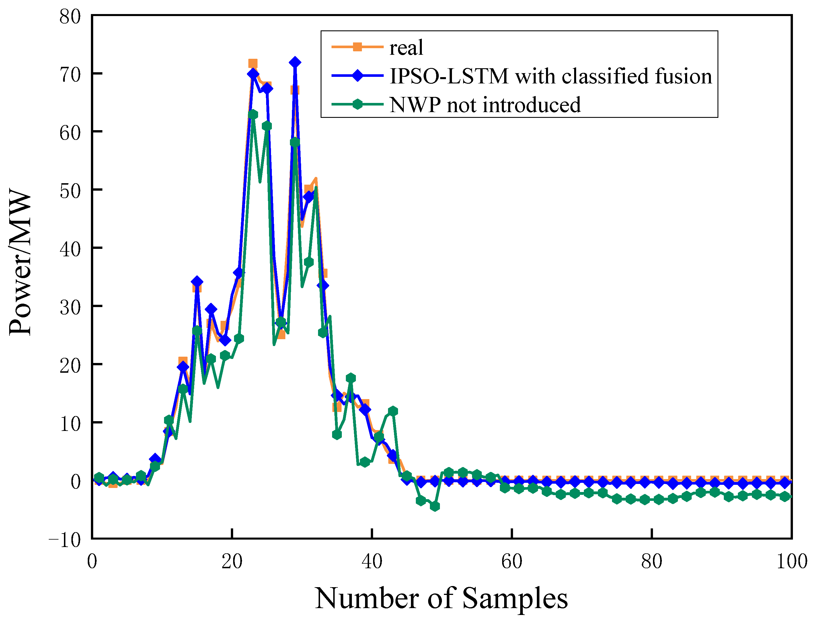
Fusion Pattern	RMSE	MAE	R2
Classified fusion	2.2842	1.4130	0.9838
Introducing NWP	10.8727	15.3512	0.9149

present the comparison between the model mentioned in this paper and the results of wind power prediction made without the use of NWP data.

As shown in Figure 15, as compared to a prediction model that just uses historical wind power data, the actual wind power curve may be more accurately predicted when NWP is included in the input data. The evaluation indices show that, in comparison to the model utilizing only historical wind power data, the RMSE and MAE of the model with the inclusion of NWP rise by 8.5885 and 13.9382, respectively, while R² lowers by 0.0689. This is because the NWP is introduced into the input data to further explore the correlation between NWP characteristics and wind power, and the NWP is used to numerically describe the trend of weather processes to further improve the predicting accuracy of wind power.

V. To verify the validity of the model proposed in this paper, the proposed model is compared and analyzed with the models reconstructed in [18,22]. The results are shown in Figure 16 and

Table 6. Evaluation indexes of the paper and the literature [18,22].

Model	RMSE	MAE	R2
Classified Fusion	2.2842	1.4130	0.9838
The literature [18]	15.3367	13.8743	0.9184
The literature [22]	17.2207	14.0842	0.9318

.

It can be seen from Figure 16 that the model proposed in this paper better fits the actual wind power curve than the other two models, and has better prediction accuracy. By comparing the evaluation indexes of the model in this paper with those in the literature [18,22], as shown in Table 6, it is be seen that the predicting accuracy of the model proposed in this paper is the highest, and its RMSE increases by 13.0525 and 14.9365, and MAE increases by 12.4613 and 12.6712, respectively, compared with the two models in the literature, and its R² decreases by 0.0654 and 0.0520, respectively. It shows that the method proposed in this paper solves the deficiencies of the models in the above literature, and greatly improves the predicting accuracy of wind power, while also further confirming the conclusion of this paper.

6. Conclusions

In order to enhance the predicting accuracy of wind power, a predicting model of wind power based on the IPSO–LSTM model and classified fusion is proposed in this paper. The simulating results with actual data show that:

(1)

In the pretreatment stage, it is necessary to decompose wind speed before prediction, which can reduce the influence of the wind speed characteristics itself on the predicting accuracy;

(2)

The improvement of w in the PSO and the addition of mutation operation in the genetic algorithm result in a difference of six orders of magnitude in the search for the extreme value of the five-dimensional sphere function, which significantly improves the globally optimal ability of the PSO, and reduces the risk of particles falling into a locally optimal solution;

(3)

The LSTM optimized by the IPSO overcomes the shortcoming of the artificially determined parameters of the LSTM, which has a better predicting effect on wind power. Moreover, compared with PSO–LSTM, the RMSE and MAE of IPSO–LSTM are decreased by 0.8776 and 0.3969, respectively, and the R² is increased by 0.0148 when using a mode of single fusion, which indicates that IPSO can obtain better parameters to optimize LSTM compared with the PSO;

(4)

The RMSE and MAE of the method of classified fusion to fuse the components of wind power decrease by 1.0460 and 0.5920, respectively, compared to those of the method of single fusion, and the R² is increased by 0.0114, which indicates that the fused accuracy of the components for wind power can be improved with the help of the method of classified fusion, and can enhance the predicting accuracy;

(5)

Compared with the literature [18,22], the RMSE of the model in this paper is increased by 13.0525 and 14.9365, the MAE is increased 12.4613 and 12.6712, and the R is decreased by 0.0654 and 0.0520, respectively, which further verifies that the model in this paper greatly improves the prediction accuracy of wind power, and the proposed optimal framework of iterative can effectively acquire the best classification model of fusion pattern and corresponding fusion model.

References

- Zhang, Y.; Sun, H.; Guo, Y. Wind Power Prediction Based on PSO-SVR and Grey Combination Model. IEEE Access 2019, 7, 136254–136267. [Google Scholar] [CrossRef]
- Zhu, A.; Zhao, Q.; Wang, X.; Zhou, L. Ultra-Short-Term Wind Power Combined Prediction Based on Complementary Ensemble Empirical Mode Decomposition, Whale Optimisation Algorithm, and Elman Network. Energies 2022, 15, 3055. [Google Scholar] [CrossRef]
- Liu, F.; Li, R.; Dreglea, A. Wind Speed and Power Ultra Short-Term Robust Forecasting Based on Takagi–Sugeno Fuzzy Model. Energies 2019, 12, 3551. [Google Scholar] [CrossRef] [Green Version]
- Blazakis, K.; Katsigiannis, Y.; Stavrakakis, G. One-Day-Ahead Solar Irradiation and Windspeed Forecasting with Advanced Deep Learning Techniques. Energies 2022, 15, 4361. [Google Scholar] [CrossRef]
- Liu, B.; Zhao, S.; Yu, X.; Zhang, L.; Wang, Q. A Novel Deep Learning Approach for Wind Power Forecasting Based on WD-LSTM Model. Energies 2020, 13, 4964. [Google Scholar] [CrossRef]
- Sun, Y.; Li, Z.; Yu, X.; Li, B.; Yang, M. Research on Ul-tra-Short-Term Wind Power Prediction Considering Source Relevance. IEEE Access 2020, 8, 147703–147710. [Google Scholar] [CrossRef]
- Bochenek, B.; Jurasz, J.; Jaczewski, A.; Stachura, G.; Sekuła, P.; Strzyżewski, T.; Wdowikowski, M.; Figurski, M. Day-Ahead Wind Power Forecasting in Poland Based on Numerical Weather Prediction. Energies 2021, 14, 2164. [Google Scholar] [CrossRef]
- He, X.; Nie, Y.; Guo, H.; Wang, J. Research on a Novel Combination System on the Basis of Deep Learning and Swarm Intelligence Optimization Algorithm for Wind Speed Forecasting. IEEE Access 2020, 8, 51482–51499. [Google Scholar] [CrossRef]
- Zhang, Y.; Zhao, Y.; Gao, S. A Novel Hybrid Model for Wind Speed Prediction Based on VMD and Neural Network Considering Atmospheric Uncertainties. IEEE Access 2019, 7, 60322–60332. [Google Scholar] [CrossRef]
- Banik, A.; Behera, C.; Sarathkumar, T.V.; Goswami, A.K. Uncertain wind power forecasting using LSTM based prediction interval. IET Renew. Power Gener. 2020, 14, 2657–2667. [Google Scholar] [CrossRef]
- Medina, S.V.; Ajenjo, U.P. Performance Improvement of Artificial Neural Network Model in Short-term Forecasting of Wind Farm Power Output. J. Mod. Power Syst. Clean Energy 2020, 8, 484–490. [Google Scholar] [CrossRef]
- Hu, T.; Wu, W.; Guo, Q.; Sun, H.; Shi, L.; Shen, X. Very short-term spatial and temporal wind power forecasting: A deep learning approach. CSEE J. Power Energy Syst. 2020, 6, 434–443. [Google Scholar]
- Xu, L.; Mao, J. Short-term wind power forecasting based on Elman neural network with particle swarm optimization. In Proceedings of the 2016 Chinese Control and Decision Conference (CCDC), Yinchuan, China, 28–30 May 2016; pp. 2678–2681. [Google Scholar]
- Lin, K.-P.; Pai, P.-F.; Ting, Y.-J. Deep Belief Networks with Genetic Algorithms in Forecasting Wind Speed. IEEE Access 2019, 7, 99244–99253. [Google Scholar] [CrossRef]
- An, G.; Jiang, Z.; Cao, X.; Liang, Y.; Zhao, Y.; Li, Z.; Dong, W.; Sun, H. Short-Term Wind Power Prediction Based on Particle Swarm Optimization-Extreme Learning Machine Model Combined with Adaboost Algorithm. IEEE Access 2021, 9, 94040–94052. [Google Scholar] [CrossRef]
- Saeed, A.; Li, C.; Danish, M.; Rubaiee, S.; Tang, G.; Gan, Z.; Ahmed, A. Hybrid Bidirectional LSTM Model for Short-Term Wind Speed Interval Prediction. IEEE Access 2020, 8, 182283–182294. [Google Scholar] [CrossRef]
- Li, A.; Cheng, L. Research on A Forecasting Model of Wind Power based on Recurrent Neural Network with Long Short-term Memory. In Proceedings of the 2019 22nd International Conference on Electrical Machines and Systems (ICEMS), Harbin, China, 11–14 August 2019; pp. 1–4. [Google Scholar]
- Sun, Z.; Zhao, S.; Zhang, J. Short-Term Wind Power Forecasting on Multiple Scales Using VMD Decomposition, K-Means Clustering and LSTM Principal Computing. IEEE Access 2019, 7, 166917–166929. [Google Scholar] [CrossRef]
- Sun, Z.; Zhao, M. Short-Term Wind Power Forecasting Based on VMD Decomposition, ConvLSTM Networks and Error Analysis. IEEE Access 2020, 8, 134422–134434. [Google Scholar] [CrossRef]
- Meng, A.; Ge, J.; Yin, H.; Chen, S. Wind speed forecasting based on wavelet packet decomposition and artificial neural networks trained by crisscross optimization algorithm. Energy Convers. Manag. 2016, 114, 75–88. [Google Scholar] [CrossRef]
- Wu, Z.; Wang, B. An Ensemble Neural Network Based on Variational Mode Decomposition and an Improved Sparrow Search Algorithm for Wind and Solar Power Forecasting. IEEE Access 2021, 9, 166709–166719. [Google Scholar] [CrossRef]
- Bo, H.; Niu, X.; Wang, J. Wind Speed Forecasting System Based on the Variational Mode Decomposition Strategy and Immune Selection Multi-Objective Dragonfly Optimization Algorithm. IEEE Access 2019, 7, 178063–178081. [Google Scholar] [CrossRef]
- Gu, D.; Chen, Z. Wind Power Prediction Based on VMD-Neural Network. In Proceedings of the 2019 12th International Conference on Intelligent Computation Technology and Automation (ICICTA), Xiangtan, China, 26–27 October 2019; pp. 162–165. [Google Scholar]
- Dong, W.; Sun, H.; Li, Z.; Zhang, J.; Yang, H. Short-Term Wind-Speed Forecasting Based on Multiscale Mathematical Morphological Decomposition, K-Means Clustering, and Stacked Denoising Autoencoders. IEEE Access 2020, 8, 146901–146914. [Google Scholar] [CrossRef]
- He, D.; Shen, S.; Wang, H.; He, Y.; Lin, Z. Wind Farm Combined Forecasting Method Based on Wavelet Packet Decomposition-new PSO-Elman Neural Network. In Proceedings of the 2019 IEEE 4th Advanced Information Technology, Electronic and Automation Control Conference (IAEAC), Chengdu, China, 20–22 December 2019; pp. 534–537. [Google Scholar]
- Zhang, S.; Zhen, Z.; Wang, F.; Li, K.; Qiu, G.; Li, Y. Ultra-Short-Term Wind Power Forecasting Model Based on Time-Section Fusion and Pattern Classification. In Proceedings of the 2020 IEEE/IAS Industrial and Commercial Power System Asia (I&CPS Asia), Weihai, China, 13–16 July 2020; pp. 1325–1333. [Google Scholar]
- Ye, R.; Guo, Z.; Liu, R.; Liu, J. Short-term wind speed forecasting method based on wavelet packet decomposition and improved Elman neural network. In Proceedings of the 2016 International Conference on Probabilistic Methods Applied to Power Systems (PMAPS), Beijing, China, 16–20 October 2016; pp. 1–6. [Google Scholar]
- Li, J.; Geng, D.; Zhang, P.; Meng, X.; Liang, Z.; Fan, G. Ultra-Short Term Wind Power Forecasting Based on LSTM Neural Network. In Proceedings of the 2019 IEEE 3rd International Electrical and Energy Conference (CIEEC), Beijing, China, 7–9 September 2019; pp. 1815–1818. [Google Scholar]
- Wang, S.; Chen, C. Short-Term Wind Power Prediction Based on DBSCAN Clustering and Support Vector Machine Regression. In Proceedings of the 2020 5th International Conference on Computer and Communication Systems (ICCCS), Shanghai, China, 15–18 May 2020; pp. 941–945. [Google Scholar]
- Makhloufi, S.; Debbache, M.; Boulahchiche, S. Long-term Forecasting of Intermittent Wind and Photovoltaic Resources by using Adaptive Neuro Fuzzy Inference System (ANFIS). In Proceedings of the 2018 International Conference on Wind Energy and Applications in Algeria (ICWEAA), Algiers, Algeria, 6–7 November 2018; pp. 1–4. [Google Scholar]