1. Introduction
According to the European Commission [
1], wave energy is considered part of the future energy mix. Many concepts of wave energy converters (WECs) have been developed [
2,
3,
4], which transform the oscillatory motion of waves into electricity. However, the development of WECs has not yet reached a commercial scale. Especially, the survivability in extreme weather conditions must be proved, and efforts must be taken to reduce the levelized cost of energy (LCOE), which is currently high compared to offshore wind and other renewable energy technologies [
5,
6]. In the design stage of a WEC, the extreme response and loads need to be well-understood to mitigate the risk of device and mooring failure. In particular, the underestimation of extreme loads can lead to the failure of critical components resulting in high repair cost, whereas an overestimation contributes to higher structural costs.
The interaction of a WEC with high and steep waves involves large amplitude structural response and nonlinear dynamics. Potential flow methods are a standard approach to model wave–structure interactions; however, it can only be applied when small amplitude and nonsteep waves are considered [
7]. For a deeper analysis in extreme wave conditions, high-fidelity computational fluid dynamics (CFD) codes are widely employed to provide accurate evaluation of the dynamics of WEC mechanisms by capturing viscous effects, wave breaking, slamming, overtopping, and large amplitude motions. The most widely used CFD-based approach is the incompressible two-phase Reynolds averaged Navier-Stokes simulations [
8], implemented in several recent studies [
9,
10,
11,
12,
13,
14].
Digital twin (DT) technology is a major asset in the hands of engineers and currently poses a huge trend in many areas, because of its capabilities, enabling the implementation of the fourth industrial revolution (Industry 4.0); however, many definitions of DT can be found in the literature [
15,
16,
17]. As defined by [
18] “
a digital twin is a virtual representation of a system or asset that calculates system states and makes system information available, through integrated models and data, with the purpose of providing decision support over its life cycle.” According to Grieves [
19], the DT constitutes three components: a physical product, a virtual representation of the product, and the interconnection between the physical and virtual states. This last component means that the virtual model is fed with data obtained from the physical product, while the information and processes from the virtual representation are the input to the physical. As stated by [
20], in many sectors, there is a need to build approaches that will help not only in the initial stages of the design process of a product but also during the operation phase [
21]. While in the initial phase, numerical simulation tools and lab-scale experiments are necessary; in the operational phase, the availability of real data bring advancements in the monitoring and improving operations during the life cycle of a product. During the last five years, an increasing interest for DT has been noticed in several fields in academia and industry [
22], bringing the DT among the most promising technology trends according to [
23].
In this work, we study a point-absorber WEC subjected to extreme wave conditions. The device consists of a surface buoy connected to a direct-driven linear generator via a taut-mooring system. The mooring force of the WEC is usually studied using CFD simulations; however, it demands high computational cost, which is leading to time-consuming solutions that are characterized by low flexibility and adaptability. This is due to the nature of CFD simulation, which is dominantly used for the WEC design, where when you change even one single parameter, new CFD simulation has to be performed, increasing the total cost of the solution and making it nonsustainable. In our application, a DT model is implemented with the purpose to eliminate the demand for numerous, time-consuming, and expensive CFD simulations during the design stage of a WEC. The DT developed in the current research work aims to model the mooring force of the WEC. In this way, the prediction of the mooring force can be obtained with less computational cost and saving valuable engineering time. The use of such a DT model will not only reduce the design time for WEC mechanisms but also increase the quality of the designed WECs. The DT methodology used in the current paper was adopted from the manufacturing domain, and it was developed and implemented by Psarommatis [
24]. The DT utilizes the ANOM statistical procedure together with data sets produced by the CFD code. This DT methodology was used due to its simplicity and minimum amount of training data. The force in the mooring line is predicted at different sea states and for alternating power take-off (PTO) characteristics. It is important to mention that this study relies on realistic values for a full-scale WEC. The wave characteristics are obtained from the 50 years environmental contour of the Dowsing study site in North Sea while realistic values are chosen for the PTO characteristics.
The main motivation of this work is the effort to minimize the required computational cost for the accurate prediction of the mooring force during extreme waves. The fast and accurate predictions of the mooring forces in extreme waves will be a valuable tool in the hands of WEC designers. As it has been previously stated, the CFD codes provide high-fidelity results, but they demand high computational cost and, in many cases, access to high-performance computing (HPC) clusters, which constitutes an additional economic cost. The DT model is trained and validated based on CFD data and produces accurate results for a fraction of the computational cost required for the CFD model to provide the same results. Therefore, the proposed DT will emulate the CFD simulation model; in other words, we propose a metamodel of the physical WEC system. To the best of knowledge of the authors, it is the first time a similar digital twin model has been presented in the wave energy field.
The paper is organized as follows. In
Section 2, a literature review is performed to explain the current status of the domain and reveal the research gap that the current paper aims to fulfill. In
Section 3, we present the wave energy concept, and the CFD model that was used.
Section 4 is devoted to the presentation of the developed DT method. In
Section 5, the predictions from the DT model and the evaluation of its performance are presented. The results are further discussed in
Section 6, and conclusions are presented in
Section 7.
2. State of the Art
In [
20], the authors present the state-of-the-art for the DT technology applied in five diverse application areas: (a) health, (b) meteorology, (c) manufacturing and process technology, (d) education, and (e) cities, transportation, and the energy sector. In order to adapt the DT concept to the wave energy sector, it is fundamental to understand the contribution of DT to offshore marine and energy systems. The first recommended practice on how to build and assure the quality of digital twins for the oil and gas industry was recently published by DNV [
18]. In the shipping industry, a DT can model a ship and estimate important parameters for the ship performance—for instance, the added resistance in waves [
25] and facilitation of monitoring and control capabilities [
26]. In the wind energy sector, a DT can coordinate work of different actors and contribute to increasing sustainability of wind energy systems in a way that addresses complex, societal, spatial, and environmental issues [
27]. DT models can be used to determine and optimize factors that reduce the LCOE of wind energy technologies, thereby improving the competitiveness of the wind energy sector. In the design stage, the DT is mirroring the performance of wind turbine based on physical methods. Techniques for modeling the wind turbine components, with varying model fidelity and computational loads, are reviewed by [
28]. During the operation stage, the structural reliability of offshore wind substructures is updated based on new information from the DT [
29]. In particular, the information is used to quantify and update the uncertainties associated with the structural dynamics and load modeling parameters in fatigue damage accumulation. In [
30], the authors utilized the DT concept to predict the axial tension in the mooring lines of a floating offshore wind turbine (FOWT). In particular, two DT models were developed; the first DT predicted the behavior of the healthy system and compared with the actual one, so as to detect long-term drifts in the mechanical response of the mooring lines. The second DT was able to predict the near-future axial tension in the mooring lines of the FOWT as a way to improve the lifespan of the mooring lines and the safety of FOWT maintenance operations. In [
31], a DT-based method was developed to predict the remaining useful life time of an offshore wind turbine by accounting medium- and short-term thermal transient loads together with long-term thermal loads. In [
32], the current practices were reviewed for the reliability analysis of the offshore wind turbines, and a DT framework applied to the support structures was proposed.
The DT models found in the literature are often categorized into physics-based models and data-driven models [
33]. In the former, the DT requires the mechanistic knowledge of the behavior of the system; thereby, the system is modeled based on the underlying equations and the mathematical analog is included. In the latter, the DT learns the behavior based on input–output examples without prior knowledge of the physical behavior of the system. Data are obtained from real measurements or numerical modeling of the system. For the learning process, machine learning (ML), artificial neural networks (ANN), or other statistical models are implemented. In this study, the analysis of means (ANOM) [
34] and additive models [
35] are considered. Authors in [
36] presented the first-ever computerized replica of a furnace that is used for flameless combustion. To create physics-based, reduced-order models for the prediction of combustion data in uncharted operating conditions, an approach combining data compression via proper orthogonal decomposition and interpolation via Kriging was created.
As discussed above, the DT technology has been successfully applied in several sectors, and the potential benefits of using DT methods in the wave energy sector are significant. In the design stage, wave energy systems typically require complex and computational expensive numerical models, especially when survivability and control aspects are to be assessed. In practice, CFD simulations are a fundamental part of the design process of a WEC because the nonlinear phenomena can be captured with good accuracy. However, they demand high computational cost and access to high performance computing (HPC) clusters, which puts a limit on the number of simulations available to the developer [
37]. When designed properly, DTs can be used in these applications to replace or complement time-consuming and costly numerical simulations or physical experiments otherwise required to analyze the system behavior [
38]. The capabilities of the DT concept are not restricted only to the design stage. The DT concept can be utilized during the offshore operation of a WEC for monitoring and predicting the response of the system based on historical examples. That is to say, the performance of the system and the integrity of critical components can be evaluated, catastrophic failures can be prevented, and the lifetime of the system might be expanded. For instance, when the weather conditions and the response of the WEC are known prior, control strategies can prevent the device exposure in extreme loads or act so as to increase the performance of the wave energy system.
Several large research projects have been started recently with the aim to model wave energy systems or predict data useful for wave energy using digital twins. In the USA, Sandia National Laboratories has partnered with Evergreen Innovations and Oregon State University to develop a DT model that captures the dynamics of the Floating Oscillating Surge Wave Energy Converter. In December 2021, the EU-funded project Integrated Digital Framework for Comprehensive Maritime Data and Information Services (ILIAD) was launched [
39]. The project aims to develop and demonstrate the use of DTs in ocean modeling and involves both nonprofit organizations such as WavEC Offshore Renewables and wave energy developers such as the Swedish/Israeli company Eco Wave Power. To support technology optimization and cost reduction engineering, the tidal energy company Orbital Marine Power in collaboration with Black & Veatch have developed a DT for their turbine [
40]. These ongoing projects show the need in marine energy research to develop digital twins and use these as fast and reliable methods to model and optimize the systems.
Despite the recent attention that has been given to incorporate evolutionary methods in the modeling of wave energy systems, few works have been published to date. Artificial intelligence (AI) algorithms and Internet of Things (IoT) were proposed as tools to analyze the many parameters influencing the performance of the WEC. As example, an IoT model equipped with an extreme machine learning algorithm was developed to monitor a WEC system and provided good prediction accuracy [
41]. For the prediction of the wave energy potential, ANN methods have been implemented. For example, a powerful ANN tool was developed and compared for the prediction the wave energy potential in nearshore coastal areas based on real measurements and the state-of-art spectral numerical model [
42]. For the estimate of important hydrodynamic coefficients, an ANN was created to predict the reflection coefficient of a submerged breakwater, and it was successfully validated based on experimental data [
43]. Model-free ANN methods were developed and applied to control of wave energy arrays by [
44,
45], and several other approaches of using model-free reinforcement learning techniques in wave energy systems have recently been published [
46,
47,
48]. Even if these works have not used the concept of DTs, they share the common idea of modeling or optimizing wave energy systems using innovative and model-free machine learning techniques.
3. Wave Energy Converter and CFD Model
In this study, a point-absorber WEC is investigated based on the concept developed at Uppsala University, Sweden. The WEC consists of a floating buoy connected to a direct-driven linear generator located at the seabed (see
Figure 1). The energy of the ocean waves is captured by the buoy motion and the PTO converts the mechanical motion to electricity. The PTO comprises a translator (T) moving vertically within the stator (S) and the alternating magnetic field induces electricity in the stator windings. The translator is pulled upwards by the buoy motion and downwards by its own weight and is restricted to move within a limited stroke length. End-stop springs are mounted at the upper and lower position of the PTO to dampen the forces on the generator hull when the translator reaches the higher and lower position. The point-absorber WEC concept ensures robustness and effectiveness during the operation. The amount of moving parts and expensive technology is minimized, and this reduces the risk of failure and the cost of offshore maintenance.
During storms and other extreme environmental conditions, high wave loads impact the operation of the system; therefore, the survivability plays a key role for the industrial development of the wave power technology. The PTO is concealed underneath the water surface. However, the buoy together with the connection line are the parts of the WEC directly affected by the extreme wave forces.
3.1. CFD Model
3.1.1. Numerical Methods
The Reynolds averaged Navier–Stokes (RANS) equations, describing the motion of an incompressible and isothermal Newtonian fluid, are expressed via the conservation of mass (Equation (1)) and momentum (Equation (2)):
where
V denotes the three-dimensional velocity field,
ρ is the density of the fluid,
p is the pressure of the fluid,
S is the viscous stress tensor, and
fb includes the external forces.
For the purpose of the present study, the open source CFD code OpenFOAM, version 1906, was utilized. The cell-centered finite volume method is implemented to solve RANS for two incompressible fluids, i.e., air and water. The free water surface is captured using the volume of fluid method (
VOF), as described by [
49]. The phase fraction, α, is used to indicate the mixture between air (
α = 0) and water (
α = 1). The two-phase problem is treated as a single fluid and the local properties (density,
ρ, and dynamic viscosity,
m) are calculated from:
The conservation of the phase fraction is essential, and an additional equation should be added to describe the motion of the phases:
where the last term is an artificial compression term and
Vc = min[
cα|
V|, max(|
V|)], where
cα = 1. The MULES algorithm is implemented to ensure that
α [0, 1] and the interface compression scheme is used to maintain sharp interfaces during the CFD simulation.
The effects of turbulence are included in the current simulations, utilizing the
k-ωSST turbulence model as suggested by [
50]. Two new transport equations are introduced:
k for the turbulent kinetic energy and
ω for the specific dissipation rate. The pressure–velocity coupling is implemented through the PIMPLE algorithm. The
overInterDyMFoam is the solver for two incompressible, isothermal fluids using
VOF method for interface capturing.
3.1.2. Force Modeling
The point-absorber WEC is modeled as a floating rigid body moored to a fixed position, allowed to move in 6 degrees of freedom. The buoy is connected with the generator via the connection line, securing coupled motion with the translator. In the model, the generator is substituted by a restraint, which represents the connection line or mooring force, Fline, acting on the buoy, and it points toward the fixed anchoring position.
The Fline is the sum of the forces applied by the generator, consisting of the translator weight, the generator damping force Fdamping, and the force due to the compression of the upper and lower end-stop springs. In later generations of the Uppsala University WEC, only an upper end-stop spring is used, Fspring, and the same setting will be used in this work. The spring force appears once the translator exceeds the upper free stroke length and hits the upper end-stop spring. When the upper spring is fully compressed, the connection line acts as an elastic cable, which adds further force, Fadd, to the system. The generator damping force, Fdamping, varies according to the generator velocity. Once the translator exceeds the lower free-stroke length, it rests at the lower position of the generator hull with the connection line being slack, leading to the uncoupled buoy–translator motion.
The total forces acting on the buoy consist of the hydrodynamic force due to wave–structure interaction, the buoy weight, and the force due to the connection line (mooring) force,
Fline, as described above. In summary, the dynamics of the buoy and the generator are described by the coupled equations of motion:
where
mb is the mass of the buoy, and
r is the position vector of the buoy. The equations are applied in the CFD simulation by an in-house developed restraint, capturing the physical behavior of the system. The line force
Fline should always point downward; otherwise, it is set equal to zero. In other words, the line can never push the buoy away, only pull the buoy toward the generator. The generator damping force,
Fdamping, is determined as:
where γ is the generator damping coefficient and
uthres is a velocity threshold. The spring force,
Fspring, is nonzero when the translator exceeds the free-stroke length, and the additional elastic line force,
Fadd, is nonzero when the translator exceeds total stroke length (free stroke length + spring length):
where
kspring and
kmooring is the spring and mooring line stiffness, respectively, and
rrest is the line length when the buoy is resting when the water level is still. When the translator exceeds the downward stroke length, the line slacks. This is implemented through the
δdown function.
Table 1 provides the physical properties of the WEC in the present study. The buoy has a cylindrical shape
3.1.3. Computational Domain
In this study, the numerical wave tank (
NWT) presented by [
10] is adapted.
Figure 2 shows the schematic view as well as the dimensions of the
NWT. The spatial discretization follows the mesh convergence study presented by [
10], which utilized the procedure of least squares fits to power series expansions, as presented by [
51]. The best error estimate is based on the standard deviation of the fits and then the error is converted into discretization uncertainty. Four cases with increasing resolution were examined. The resolution was defined as parametric as the ratio of the maximum crest amplitude to the cell size (
Ap/Δ
z). The study reveals that monotonic convergence is observed and the ratio can be taken equal to
Ap/Δ
z = 17. For this choice, the inferred discretization uncertainty is less than 1%. The cells are kept orthogonal (Δ
x = Δ
y = Δ
z) in the refined region close the water surface to generate wave with better shape.
Figure 2 also shows the enlarge area around the WEC where one can see the refined region with height of 2
Ap, the one level lower refinement region of 2
Ap, and the overset mesh. The overset dynamic mesh technique was utilized due to the extreme wave nature and the expected great structural response. The overset mesh is a cubic area surrounding the floating body with high resolution, almost equal to the resolution of the refined region in the water surface. The authors have utilized the overset method in several studies [
9,
10,
12]. Due to the utilization of
k-ω SST turbulence model, wall functions are adapted to solve the boundary layer. Therefore, good discretization is required around the WEC. The
y+ is kept within the range of [30, 300] as stated by [
50].
The IHFOAM toolbox is implemented in OpenFOAM v1906 and utilized for the wave generation and absorption. This study considers focused wave groups based on the NewWave theory [
52]. The number of wave components the focused wave consists of is selected based on the study conducted by [
10].
The dynamic motion of the WEC is accommodated using the overset dynamic mesh method. The PTO system, as described in Section entitled “Force modeling”, is implemented in OpenFOAM using a numerical restraint. In particular, the sixDoFRigidBodyMotion library solves the 6 degrees of freedom body motion based on Newton’s second law. The forces and moments due to wave–structure interaction and the additional external forces, i.e., the PTO numerical restraint, are considered for the motion estimate.
For the solution, the variable time step was adjusted to the Courant–Friedrichs–Lewy (CFL) condition of maximum CFL number 0.5. The size of cells varies depends on the wave characteristics of the examined wave; therefore, the number of computational cells varies from 6 × 10⁶ to 31 × 106 cells. All the cases were run on the Tetralith HPC cluster using 128 processors. Each case can utilize 3584–11,776 CPU hours, depending on the number of computational cells.
4. Digital Twin Method
The mooring system is a critical mechanical component for the studied taut-moored point-absorber WEC as it is the only element connecting the buoy with the PTO. Any failure can be catastrophic for the performance of the WEC. Extreme loads and fatigue are the primary causes for the failure of the mooring system [
53]. The purpose of this work is to create an accurate DT model able to predict the force in the mooring line of a WEC when subjected to extreme waves. The current DT is developed using a standardized methodology for DT development presented in [
54], which was also followed in [
24].
In this section, the general procedure for the development and validation of the DT is explained.
Figure 3 illustrates the steps of the procedure and how they are connected. More detailed analysis of each step is found in the following sections.
Step 1. Selection of DT input parameters. The initial step is the identification of the DT input parameters, alongside the corresponding value range for each input parameter. These parameters are the ones mainly affecting the behavior of the mooring force. Detailed analysis is found in the Section entitled “Selection of the input parameters”.
Step 2. Design and training of the DT model. The DT provides the output prediction utilizing a mathematical model based on the statistical developed by [
24]. The definition of the training data sets is based on the design of experiments (DoE) method as defined by the Taguchi approach [
35]. Once the range of input parameters has been selected, the most suitable orthogonal array is defined. As this study focuses on extreme waves, a high-fidelity CFD model is expected to provide an accurate estimate. However, this choice poses the restraint of limited simulations due to high computational cost. As a compromise between sufficiently many simulations to provide enough training data and feasible computational cost for the CFD simulations, 25 tests will be conducted based on the L25 orthogonal array. The CFD simulations are conducted based on those experiment sets. The results are then utilized to train the DT model.
Step 3. Validation of the DT model. Once the DT is trained, its capability to accurately predict the output (i.e., the mooring force) has to be tested. For that reason, a new set of data is selected for testing purposes. In this study, 50 test data sets are randomly chosen. Again, CFD simulations are performed to estimate the mooring force for the testing cases. As a last step, the results obtained from the DT model for the testing data are compared with the CFD solution. An error analysis is necessary to obtain a quantitative measure of the agreement between the prediction and the solution.
4.1. Selection of the Input Parameters
As described in Section “Overview of the procedure”, the first step in digital twin design is to define the input parameters. In the current case study, four input parameters were selected:
Significant wave height, Hs [m]
Wave peak period, Tp [s]
PTO damping coefficient, γ [N]
PTO upper end-stop spring stiffness, kspring [N/m]
Further discussion about the physical meaning of the input parameters is provided below in this Section and in the Section entitled “Force modeling”.
As previously discussed, the mooring line is a critical mechanical component for the operation and survivability of the WEC; therefore, the force in the mooring line is selected as the output parameter of the DT model. The mooring line force heavily depends on the sea state and the PTO characteristics, justifying the selection of the input parameters.
Extreme wave selection: In offshore renewable energy engineering, a common practice for the selection of the design waves relies on the 50-year return period environmental contour for a particular study site [
55]. This approach has been considered by many authors [
9,
56,
57,
58,
59]. In our study, the environmental contour for the Dowsing site, shown in
Figure 4, is utilized for the wave selection. The Dowsing site is located in the North Sea, 56 km from the west coast of the United Kingdom, with water depth of 22 m. The same location has been considered in previous studies, also with the focus of extreme wave characterization and survivability [
10,
58].
The sea states selected for the training stage of the DT model are characterized by significant wave height,
Hs, and peak period,
Tp, with range of values along and inside the environmental contour line
Figure 4. Therefore, the assigned ranges for these parameters are:
Hs = 2.5–6.8 m and
Tp = 8.3–14.1 s (
Table 2).
In the numerical simulations, modeling the extreme wave conditions with a random wave series is a demanding process and requires much computational time. A common approach is to represent the extreme wave as a focused wave group, which is the superposition of many small amplitude waves. The physical process close to the focusing point, where the peak amplitude occurs, is highly nonlinear due to the complex wave components interactions resulting in the presence of the extreme loads. The focused wave is a popular approach for extreme wave simulation utilized in this study. In particular, the focused waves were modeled here according to the NewWave theory [
52]. The extreme waves are further characterized by the wave steepness,
KpAp, provided in
Table 3 and
Table 4 as an additional information. However, the wave steepness does not constitute an input parameter to the DT model.
PTO characteristics: the values for the generator damping,
γ, and the upper end-stop stiffness,
kp, are selected based on values utilized in previous studies [
9,
10,
12]. For the training stage of the DT model, the specific values of these parameters are found in
Table 2.
4.2. Digital Twin Construction
In this section, the utilized methodology for the DT construction was first introduced by [
24] in the manufacturing domain with the goal to design a manufacturing system to achieve zero-defect manufacturing [
60,
61]. In particular, the DT emulated a dynamic scheduling tool with the goal to minimize the computational time. This method was selected for the current application because it is lean, has a high level of accuracy, requires few data points for training the DT model, and is aligned with the motivation of this paper. In this work, the DT aims to predict the dynamic mooring force of the WEC system presented in the Section entitled “Wave Energy Converter”. The force is calculated based on computationally expensive CFD simulations; therefore, the main goal is to predict the mooring force without the need for running the CFD code.
The procedure is based on the statistical method of design of experiments (DoE) as defined by the Taguchi approach [
35]. The selected method can capture the individual effects of each input parameter, facilitate the minimization of the required training experiments, and determine the exact experiments. To capture the effects of each parameter, an orthogonal array allows us to consider a selected subset of combinations of multiple input parameters at multiple values. The orthogonal arrays are balanced to ensure that all the values of all the input parameters are considered equally and evaluated independently. For this application, an L
25 orthogonal array is used offering high resolution, examining five values for each input parameter. As a result, the L
25 implies that 25 CFD simulations are required to create the digital twin.
Once the experiments have been completed, the analysis of the results follows.
Figure 5 summarizes the steps for analyzing the CFD results and constructing the DT of the CFD model. At the first step, the overall mean, μ, of the mooring force (MF) for the 25 experiments is calculated (Equation (12)). At the second step, the analysis of means (ANOM) methodology is implemented to capture the contribution of each value of each input parameter to the MF, thereby, 20 ANOM coefficients are calculated (Equation (13)). The third step finds the effect of each parameter to the MF based on the overall mean and the ANOM coefficient (Equation (14)) where N is the number of the experiments (
N = 25),
R is the number of input values (
R = 5), and the subscripts f and z declare the input parameter and the value, respectively.
At the fourth step, the statistical analysis of the CFD data is utilized to construct the desired model for predicting the dynamic MF. From the analysis, the discrete values are available and represented in the Cartesian system, as shown in
Figure 5, plot A. The contribution of each parameter to the total MF is the matrix presented in Equation (15) (e.g.,
F1(
Hs1) =
f11,
F2(
Tp1) =
f21,
F3(
γ1) =
f31,
F4(
kspring1) =
f41, etc.). The matrix defined in Equation (16) summarizes the values of each input parameter. The two matrices are combined and form the Cartesian points (Equation (17)).
At this step, it is necessary to move from the discrete points to the continues model. A piecewise spline interpolation is performed through the discrete points resulting in a third order polynomial model, Equation (19). Here, the coefficients
q,
s,
t, and
l are calculated from the MATLAB “
fit” function. As an example, for the reader, for predicting the continues model for the input parameter
Hs, the matrix of Equation (19) takes the form of Equation (20). The continues model is shown in
Figure 5, plot B. The repetition of the previous steps (step 2–4) will result to a set of four graphs with the continuous input parameter effects (step 5). The final step (step 6) integrates all the results to one single model (Equation (18)) that is able to predict the dynamic mooring force, as CFD simulations would calculate, for any set of input parameter values. Furthermore, the effect of each individual input parameter is reflected on the mooring force.
4.3. Training Procedure
In this section, we will analyze how the digital twin methodology will be applied to the current examined case.
Table 2 presents the values for each of the four input parameters. Those values are carefully selected to represent reality and be as generic as possible in order for the developed digital twin model to be flexible and to be able to calculate a high variety of wave and mechanism situations. Based on the L
25 orthogonal array, 25 experiments are required for the creation of the digital twin model.
Table 3 presents the experimental matrix based on the L
25 and the input parameters values. The experiments will be conducted using CFD simulations as described in the next Section entitled “CFD model”.
The selected DT methodology takes as an input the DT input parameters and provides as an output the mooring force, which is one single value and not a time series of 52 s as in the output of the CFD simulation. To overcome this obstacle, multiple DT sub-models were created to represent a specific time step in the simulation. More specifically, the 52 s of the CFD simulations were discretized into time steps of 0.01 s. For each of the time steps, a DT submodel was constructed that will predict the mooring force for the specific time step. Therefore, the final digital twin model that will be produced will be a collection of 5200 models, one for each time step. This will allow to create the mooring force time series for a given set of input parameters. The development of the 5200 DT sub-models will be performed using the same data, coming from the 25 CFD simulations presented in
Table 3.
4.4. Validation Procedure
In order to test the accuracy and validate the developed digital twin, 50 new experiment sets were defined randomly; their values are shown in
Table 4. At this point, it should be mentioned that for experiments No. 1–25 all the digital twin input parameters are within the range that the digital twin was created,
Table 2, whereas No. 26–50 were selected at the end of the range and some of them outside to test the robustness of the digital twin. In this study, emphasis is given in the extreme waves; therefore, waves with higher wave height and steepness are mainly chosen for the testing purposes. The goal is to compare the mooring forces calculated from the CFD with the one from the digital twin. As described in Section entitled “Digital twin construction”, 5200 models were created, one for each time step of 0.01 s of the total 52 simulation seconds.
To measure the accuracy of the digital twin to predict the force at a given data set, the mean absolute percentage error,
ε, is used and calculated using Equation (21), where
N is the number of time steps points, i.e.,
N = 5200,
y is the value from the CFD and
is the value from the digital twin.
The procedure starts with the calculation of the relative difference between the CFD and digital twin for each one of the 5200 models/time steps. Once all the relative differences are calculated, the outliers are removed using the mean, where an outlier is defined as an element more than three standard deviations from the mean. The remaining points are summed, and the average value is calculated. The result is the average error of the digital twin. Using Equation (22), the accuracy, A, of the prediction for a particular data set is computed. The average global accuracy, , of the DT model is calculated by averaging the accuracy, A, for all the examined data sets.
5. Results
5.1. Preliminary Results
Once the 50 validation experiments were performed, the comparison between the simulated and predicted mooring force values could take place.
Figure 6 illustrates the mooring line force calculated by the CFD (with blue line) and the initial DT model (red line). Despite the fact that the DT model has a general good fit over the simulated time, there is a significant lack of fit in the three peaks in seconds ~32, ~40 and ~48. This behavior was the same for all the 50 validation experiments. The average global accuracy
of the DT model is equal to 82.45%, based on the 50 validation experiments. This lack of accuracy motivated us to modify the initial DT model and enrich it with additional models in order to fit better the peaks, using the same 25 training data points.
5.2. Results from the Enhanced Digital Twin Model2
To enhance accuracy and lack of fitness for those three peak occasions, an additional set of three DT models were added on top of the 5200 models. Using the same 25 training data sets, three extra models were developed for predicting each one of the three peaks. Then, the 5200 models and the 3 peak models were incorporated together into a MATLAB code to form one single solution.
The procedure used for the generation of the additional three models was first to find and isolate those peak values for each of the 25 initial experiments. Once those peak values were isolated, the DT methodology presented in
Figure 5 could take place for each of the three peaks. The outcome of those peak DT models will be the peak value for any set of the four defined parameters. The aggregation of those models was performed as follows. First, the initial DT (with only the 5200) creates the initial solution. Then, an algorithm searches and finds the exact time that each of the three peaks occurs and for each peak using the corresponding peak DT model and input parameters set calculates the enhanced peak value and replaces the initial one. The mooring force value of the initial DT model is then computed for two time steps ±0.45 s from the peak. Finally, using the peak value and each of the two (± 0.45 s) values, a linear interpolation is carried out to connect them. Once the linear equation is calculated, all the values between the ±0.45 s from the peak value are replaced by the values calculated by the linear interpolation. The result from this procedure is an enhanced DT model with significantly higher accuracy than the initial one.
Once the 50 validation experiments were simulated using CFD, the methodology presented in Section entitled “Digital twin construction” was used to calculate the accuracy of the digital twin. The results are presented in
Table 5 and show the accuracy of the initial (DT
initial) and enhanced (DT
ench) DTs as well as the accuracy of the additional 3 DTs, which were used to enhance the capability of the initial DT to predict more accurately the three peaks forces (Peak
1, Peak
2, Peak
3). The average global accuracy
of the enhanced DT was calculated as 90.36% by averaging the individual accuracy of the data sets No. 1–50. The average global accuracy
of the initial DT model is 82.46%, which is significantly lower than the accuracy of the enhanced DT, underlining the importance of the enhanced DT. The peaks in the mooring force are evaluated separately and the drawn conclusion is that they are predicted with high average global accuracy
in the range 83.82–91.05%. From the 3 peaks, Peak
2 is the most critical, which is always the higher force acting in the mooring line. The average global accuracy
of the Peak
2, as predicted by the enhanced DT, is 86.51%.
Figure 7 shows the scatter of the maximum peak Peak
2 for the 50 testing data sets and how they compare to the numerical solution. The Peak
2 was selected because it is the most important among the three peaks, as it always presents the maximum value corresponding to the focal time of the focused wave. The data sets are depicted with red and blue dots with the latter showing better prediction when compared with the numerical results. For the red area, the prediction accuracy drops. The reason is that the red region consists of the data sets No. 26–50 for which the significant wave height,
Hs, is greater than the range of the training data sets. That is to say, while for training the DT, the
Hs = 3.5–6.8 m, some of the testing data No. 26–50 exceed this range (
Hs > 6.8 m). This does not happen for the testing data sets No. 1–25, which are always within the range.
The results from the 50 validation experiments of the DT model are shown in
Figure 8 by six examples. Three lines are plotted, with the black dashed line showing the results from the CFD simulation, while the blue dash dot line shows the results from the initial DT and the solid red line the results from the enhanced DT model. From the results presented, one can see that the addition of the extra DT models for the peaks (enhanced DT) was crucial for the overall performance of the DT of the wave energy converter mechanism. When comparing
Figure 7 and
Figure 8, it can be noticed that the data sets No. 7, 24, and 25 of
Figure 8 belong to the results plotted in blue in
Figure 7, i.e., they have input parameter values within the range of the training data for the DT, which explains their good fit to the CFD results. Conversely, No. 28, 29, and 42 of
Figure 8 are in the red region of
Figure 7, i.e., their input parameters are outside the range of the training data, which explains the smaller accuracy for these cases.
5.3. Sensitivity to Input Parameters
As described in Section entitled “Digital twin construction”, the DT calculates the mooring force as the sum of the overall mean value, μ, and the influence effect of the wave height, wave period, PTO damping, and spring stiffness expressed as F1, F2, F3, and F4, respectively.
In this section, we will evaluate the sensitivity of the mooring force to the input parameters values. The evaluation is illustrated by means of the 3D surface plots shown in
Figure 9. For the total simulation time (52 s), the mooring force can change depending on the assigned value of the input parameters. From
Figure 9, it can be concluded that the significant wave height, H
s, has the maximum influence (
F1 = 140 kN) when
Hs > 7 m. For small values of
Hs, the mooring force is negatively affected as compared to the mean value. The wave peak period shows the maximum contribution for shorter waves,
Tp < 10 s, implying that steeper waves result in the increase of the mooring force. The contribution of wave period reaches up to
F2 = 120 KN. The influence of the PTO characteristics,
F3 and
F4, is less compared to the wave characteristics. In particular, the maximum value of
F3 is 40 kN and occurs for large damping coefficient,
γ, while the maximum value of
F4 is 30 kN and mainly appears for large spring stiffness.
As a second step of this sensitivity study, it is important to analyze how the four input parameters affect the magnitude of the maximum peak, Peak
2. As mentioned earlier, Peak
2 is critical not only for the design stage but also for the safe operation of the system.
Figure 10 shows the influence of each input parameter in Peak
2. The wave height follows a linear trend. For
Hs > 5 m, the mooring force significantly increases; otherwise, for smaller waves, the force tends to get smaller values as compared to the mean. The wave period parameter presents the minimum contribution at
Tp = 11 s. For very short waves (
Tp = 8 s) and for very long waves (
Tp > 13 s), the influence of the wave peak period increases significantly. The PTO damping coefficient contributes to the higher increase in the mooring force (
γ > 70 kN), while the stiffness of the upper end-stop spring contributes to an increasing trend for
kspring > 800 kN. In the present study, the PTO damping coefficient has been kept constant throughout each wave condition, which is consistent with a no-control or passive control approach. From the results, the PTO damping affects the experienced loads. This is consistent with earlier studies, which confirmed both experimentally [
62,
63] and numerically [
9,
64] that the extreme loads depend on the applied PTO damping. In general, while the PTO damping and the spring stiffness affect the mooring line force, the influence of the wave height is several magnitudes higher.
6. Discussion
The DT method adapted in this study has been used initially in the manufacturing domain, particularly to model a production scheduling tool [
24] with the primary goal to avoid time-consuming simulations. The motivation of the present work is also the need for a faster modeling tool compared to the traditional techniques. The findings from both studies prove high accuracy and flexibility of the method and its capability to provide successful solution to interdisciplinary applications. However, a common trend is the accuracy reduction when high fluctuations are presented. To overcome this accuracy problem, an enhanced DT was developed, improving the accuracy on areas with high fluctuations.
The main goal of the current study is to provide wave energy conversion designers a tool for fast and accurate predictions of the WEC mooring line force, increasing the efficiency and sustainability of the design process. Specifically, the developed DT model can be used in the initial steps of a WEC design process, and once the final design has been reached, a detailed CFD model can be utilized to quantify the mooring force in a higher accuracy. By following this approach, a vast amount of computational time and cost will be avoided, making the design process more sustainable and faster. Moreover, this DT model can be used as a monitoring tool for measuring the integrity of the real system, operating offshore. The results show that particular care must be taken to capture peaks in the mooring force, which has been addressed in the enhanced version of the DT model. This mainly occurred because one DT model was created for each time step of 0.01 s, yet the peaks did not occur at this exact time step; therefore, the presence of peaks was not captured well. The development and aggregation of the extra three DTs for the peaks was crucial for improving the DT accuracy. With the enhanced DT model, the average global accuracy was improved by approximately 8% while the maximum peak, Peak2, was estimated with an accuracy of 86.51%.
It is also important to state that the accuracy of the DT model increases when the input parameters are within the range of the training sample. Therefore, the selection of the training data sets is a critical step for the successful predictive capabilities of the DT. The presented method required a small number of training data points, and this is a significant advantage making its implementation feasible, practical, and easy. From this study, useful outcomes are drawn regarding the influence of the input parameters. It is concluded that the wave height has the greatest influence in the magnitude of the mooring force, while the PTO characteristics contribute less. It is noticed that for waves higher than 5 m, the force in the mooring increases significantly. The DT model gives also information about the selected values for the PTO characteristics. In this application, the PTO damping coefficient is suggested to be less than 70 kN, while the upper end-stop spring stiffness is less than 800 kN/m.
In this study, each CFD simulation demanded from 28 h up to 92 h at HPC cluster utilizing 128 processors. The DT model required only 1.34 s to provide the prediction for the mooring force. The specifications of the computer utilized for the DT development and mooring force prediction are CPU Intel Core i7 6800K @3.40GHz, memory: 32Gb RAM, GPU: NVIDIA 1080 Ti 5Gb, operating system: Windows 10. It is obvious that the DT significantly minimizes the computational cost to a fraction of time.
7. Conclusions
In this paper, we introduce a statistical model that fits the input–output behavior of the mooring system of a wave energy converter, while the model is trained based on CFD simulations. In particular, the model is able to predict the force in the mooring system of a wave energy converter subjected in extreme wave conditions and for adaptive PTO settings.
As stated in the literature, high-fidelity CFD simulations is one of the traditional approaches in the field; however, a statistical model able to fit the input–output pairs reduce the computational cost and increases the efficiency in the engineering design. Furthermore, the method presented in this study has the advantage that it does not demand a great amount of data for learning the system’s behavior. The method has been initially utilized in the manufacturing field, and now, it has been successfully implemented in the wave energy sector, highlighting the interdisciplinary benefit of the method. This is a great contribution to the ascending wave energy applications and one of the first attempts of experimental design in the wave energy structures, as to the best authors knowledge.
In our work, the average global accuracy of the model is 90.36% as compared to the CFD simulations. While the latter need from some hours up to few days to complete, even with access to high performance computing clusters, the DT model requires only a few seconds on a standard PC. However, it is important to clarify here that the contribution of CFD is still fundamental in the development of our model. Nevertheless, a considerable smaller number of CFD simulations is required to understand the system’s dynamics. Furthermore, the range of training values is crucial for the model’s uncertainty; the accuracy of the DT model reduces for inputs outside the training range.
This study provides also an interesting conclusion in terms of mooring dynamics in extreme wave conditions. For our application, the mooring force increases significantly in high (Hs > 5 m) and extreme waves, while the model gives an understanding of how to select properly the PTO characteristics in order to reduce the peaks in the mooring force.
As future work for similar applications, models based on ML and/or ANN methods are suggested; however, more data may need to be available. Furthermore, as previously mentioned, the training data sets need to be carefully selected in order to avoid excess of available training data. In practice, each data point may be expensive or demand days; therefore, it must be consciously selected. Active-learning algorithms are a suitable future approach, as they investigate regions of the input space that are seemed more relevant to the output of interest reducing the demand of large amount of data. Last, apart from the design stage, DT models are implemented for monitoring purposes and life-cycle prediction. In this case, the availability of real measurements during operational conditions would allow the construction of a realistic model of the system, which can be continuously updated.
Author Contributions
E.K.: Conceptualization of this study, methodology, CFD simulations, analysis of the results, writing and editing. F.P.: Conceptualization of this study, methodology, digital twin development, analysis of the results, writing and editing. M.G.: Analysis of the results, writing and editing. All authors have read and agreed to the published version of the manuscript.
Funding
The research in this paper was supported by the Centre of Natural Hazards and Disaster Science (CNDS), the Swedish Research Council (VR, grant number 2020-03634), the Swedish Energy Agency (project number 47264-1), the Onassis Foundation (Scholarship ID: FZP 021-1/2019-2020). Also, this paper was partially supported by EU funded project Eur3ka, under grant agreement No. 101016175. This research work reflects only the authors’ views, and the Commission is not responsible for any use that may be made of the information it contains.
Institutional Review Board Statement
Not applicable.
Informed Consent Statement
Not applicable.
Data Availability Statement
Data available on request.
Acknowledgments
The CFD simulations were performed on resources provided by the Swedish National Infrastructure for Computing (SNIC) at the HPC cluster: Tetralith at the National Supercomputer Centre, Linköping University.
Conflicts of Interest
The authors declare no conflict of interest.
References
- COM(2020)741-EU Strategy to Harness the Potential of Offshore Renewable Energy for a Climate Neutral Future-EU Monitor. Available online: https://www.eumonitor.eu/9353000/1/j9vvik7m1c3gyxp/vldwjbykscwq (accessed on 18 July 2022).
- de O. Falcão, A.F. Wave Energy Utilization: A Review of the Technologies. Renew. Sustain. Energy Rev. 2010, 14, 899–918. [Google Scholar] [CrossRef]
- López, I.; Andreu, J.; Ceballos, S.; De Alegría, I.M.; Kortabarria, I. Review of Wave Energy Technologies and the Necessary Power-Equipment. Renew. Sustain. Energy Rev. 2013, 27, 413–434. [Google Scholar] [CrossRef]
- Babarit, A. Ocean Wave Energy Conversion: Resource, Technologies and Performance. In Ocean Wave Energy Conversion: Resource, Technologies and Performance; ISTE Press: London, UK, 2017; pp. 1–262. [Google Scholar] [CrossRef]
- de Andres, A.; Medina-Lopez, E.; Crooks, D.; Roberts, O.; Jeffrey, H. On the Reversed LCOE Calculation: Design Constraints for Wave Energy Commercialization. Int. J. Mar. Energy 2017, 18, 88–108. [Google Scholar] [CrossRef]
- Rusu, E.; Onea, F. A Review of the Technologies for Wave Energy Extraction. Clean Energy 2018, 2, 10–19. [Google Scholar] [CrossRef] [Green Version]
- LeMéhauté, B. An Introduction to Hydrodynamics and Water Waves; Springer: Berlin/Heidelberg, Germany, 1976; p. 323. [Google Scholar]
- Windt, C.; Davidson, J.; Ringwood, J.V. High-Fidelity Numerical Modelling of Ocean Wave Energy Systems: A Review of Computational Fluid Dynamics-Based Numerical Wave Tanks. Renew. Sustain. Energy Rev. 2018, 93, 610–630. [Google Scholar] [CrossRef] [Green Version]
- Katsidoniotaki, E.; Göteman, M. Numerical Modeling of Extreme Wave Interaction with Point-Absorber Using OpenFOAM. Ocean Eng. 2022, 245, 110268. [Google Scholar] [CrossRef]
- Katsidoniotaki, E.; Nilsson, E.; Rutgersson, A.; Engström, J.; Göteman, M. Response of Point-Absorbing Wave Energy Conversion System in 50-Years Return Period Extreme Focused Waves. J. Mar. Sci. Eng. 2021, 9, 345. [Google Scholar] [CrossRef]
- van Rij, J.; Yu, Y.H.; Tran, T.T. Validation of Simulated Wave Energy Converter Responses to Focused Waves. Eng. Comput. Mech. 2021, 174, 32–45. [Google Scholar] [CrossRef]
- Katsidoniotaki, E.; Ransley, E.; Brown, S.; Palm, J.; Engstrom, J.; Goteman, M. Loads on a Point-Absorber Wave Energy Converter in Regular and Focused Extreme Wave Events. In Proceedings of the ASME 2020 39th International Conference on Ocean, Offshore and Arctic Engineering, Online, 3–7 August 2020; Volume 9. [Google Scholar] [CrossRef]
- Windt, C.; Davidson, J.; Ransley, E.J.; Greaves, D.; Jakobsen, M.; Kramer, M.; Ringwood, J.V. Validation of a CFD-Based Numerical Wave Tank Model for the Power Production Assessment of the Wavestar Ocean Wave Energy Converter. Renew. Energy 2020, 146, 2499–2516. [Google Scholar] [CrossRef]
- Survivability of Wave Energy Converter and Mooring Coupled System Using CFD|Semantic Scholar. Available online: https://www.semanticscholar.org/paper/Survivability-of-Wave-Energy-Converter-and-Mooring-Ransley/f4e2be03de97019885bb5121be3c1a77f1c92e27 (accessed on 22 June 2022).
- VanDerHorn, E.; Mahadevan, S. Digital Twin: Generalization, Characterization and Implementation. Decis. Support. Syst. 2021, 145, 113524. [Google Scholar] [CrossRef]
- Ruppert, T.; Abonyi, J. Integration of Real-Time Locating Systems into Digital Twins. J. Ind. Inf. Integr. 2020, 20, 100174. [Google Scholar] [CrossRef]
- Zheng, X.; Psarommatis, F.; Petrali, P.; Turrin, C.; Lu, J.; Kiritsis, D. A Quality-Oriented Digital Twin Modelling Method for Discrete Manufacturing Processes Based on a Multi-Agent Architecture. Procedia Manuf. 2020, 51, 309–315. [Google Scholar]
- DNV-RP-A204 Qualification and Assurance of Digital Twins-DNV. Available online: https://www.dnv.com/oilgas/download/dnv-rp-a204-qualification-and-assurance-of-digital-twins.html (accessed on 22 June 2022).
- Grieves, M. Digital Twin: Manufacturing Excellence through Virtual Factory Replication; Florida Institute of Technology: Melbourne, FL, USA, 2014. [Google Scholar]
- Rasheed, A.; San, O.; Kvamsdal, T. Digital Twin: Values, Challenges and Enablers from a Modeling Perspective. IEEE Access 2020, 8, 21980–22012. [Google Scholar] [CrossRef]
- Oblak, B.; Babnik, S.; Erklavec-Zajec, V.; Likozar, B.; Pohar, A. Digital Twinning Process for Stirred Tank Reactors/Separation Unit Operations through Tandem Experimental/Computational Fluid Dynamics (CFD) Simulations. Processes 2020, 8, 1511. [Google Scholar] [CrossRef]
- Jones, D.; Snider, C.; Nassehi, A.; Yon, J.; Hicks, B. Characterising the Digital Twin: A Systematic Literature Review. CIRP J. Manuf. Sci. Technol. 2020, 29, 36–52. [Google Scholar] [CrossRef]
- Top 10 Strategic Technology Trends for 2019|Gartner. Available online: https://www.gartner.com/en/newsroom/press-releases/2018-10-15-gartner-identifies-the-top-10-strategic-technology-trends-for-2019 (accessed on 22 June 2022).
- Psarommatis, F. A Generic Methodology and a Digital Twin for Zero Defect Manufacturing (ZDM) Performance Mapping towards Design for ZDM. J. Manuf. Syst. 2021, 59, 507–521. [Google Scholar] [CrossRef]
- Taskar, B.; Andersen, P. Comparison of Added Resistance Methods Using Digital Twin and Full-Scale Data. Ocean Eng. 2021, 229, 108710. [Google Scholar] [CrossRef]
- Fonseca, Í.A.; Gaspar, H.M.; de Mello, P.C.; Sasaki, H.A.U. A Standards-Based Digital Twin of an Experiment with a Scale Model Ship. Comput.-Aided Des. 2022, 145, 103191. [Google Scholar] [CrossRef]
- Solman, H.; Kirkegaard, J.K.; Smits, M.; van Vliet, B.; Bush, S. Digital Twinning as an Act of Governance in the Wind Energy Sector. Environ. Sci. Policy 2022, 127, 272–279. [Google Scholar] [CrossRef]
- de Kooning, J.D.M.; Stockman, K.; de Maeyer, J.; Jarquin-Laguna, A.; Vandevelde, L. Digital Twins for Wind Energy Conversion Systems: A Literature Review of Potential Modelling Techniques Focused on Model Fidelity and Computational Load. Processes 2021, 9, 2224. [Google Scholar] [CrossRef]
- Augustyn, D.; Ulriksen, M.D.; Sørensen, J.D. Reliability Updating of Offshore Wind Substructures by Use of Digital Twin Information. Energies 2021, 14, 5859. [Google Scholar] [CrossRef]
- Walker, J.; Coraddu, A.; Collu, M.; Oneto, L. Digital Twins of the Mooring Line Tension for Floating Offshore Wind Turbines to Improve Monitoring, Lifespan, and Safety. J. Ocean Eng. Mar. Energy 2022, 8, 1–16. [Google Scholar] [CrossRef]
- Sivalingam, K.; Sepulveda, M.; Spring, M.; Davies, P. A Review and Methodology Development for Remaining Useful Life Prediction of Offshore Fixed and Floating Wind Turbine Power Converter with Digital Twin Technology Perspective. In Proceedings of the 2018 2nd International Conference on Green Energy and Applications, ICGEA 2018, Singapore, 24–26 March 2018; pp. 197–204. [Google Scholar] [CrossRef]
- Wang, M.; Wang, C.; Hnydiuk-Stefan, A.; Feng, S.; Atilla, I.; Li, Z. Recent Progress on Reliability Analysis of Offshore Wind Turbine Support Structures Considering Digital Twin Solutions. Ocean Eng. 2021, 232, 109168. [Google Scholar] [CrossRef]
- Tao, F.; Xiao, B.; Qi, Q.; Cheng, J.; Ji, P. Digital Twin Modeling. J. Manuf. Syst. 2022, 64, 372–389. [Google Scholar] [CrossRef]
- Ryan, T.P. The Analysis of Means: A Graphical Method for Comparing Means, Rates, and Proportions. J. Qual. Technol. 2018, 38, 191–193. [Google Scholar] [CrossRef]
- Phadke, M.S. Quality Engineering Using Robust Design; Prentice Hall PTR: Hoboken, NJ, USA, 1995; ISBN 0-13-745167-9. [Google Scholar]
- Aversano, G.; Ferrarotti, M.; Parente, A. Digital Twin of a Combustion Furnace Operating in Flameless Conditions: Reduced-Order Model Development from CFD Simulations. Proc. Combust. Inst. 2021, 38, 5373–5381. [Google Scholar] [CrossRef]
- Molinaro, R.; Singh, J.S.; Catsoulis, S.; Narayanan, C.; Lakehal, D. Embedding Data Analytics and CFD into the Digital Twin Concept. Comput. Fluids 2021, 214, 104759. [Google Scholar] [CrossRef]
- Pavlišič, A.; Ceglar, R.; Pohar, A.; Likozar, B. Comparison of Computational Fluid Dynamics (CFD) and Pressure Drop Correlations in Laminar Flow Regime for Packed Bed Reactors and Columns. Powder Technol. 2018, 328, 130–139. [Google Scholar] [CrossRef]
- Home|Iliad-Digital Twin of the Ocean. Available online: https://www.ocean-twin.eu/ (accessed on 22 June 2022).
- Orbital Marine Power Teams Up with Black & Veatch for Tidal Turbine Optimisation-Orbital Marine. Available online: https://orbitalmarine.com/orbital-marine-power-teams-up-with-black-veatch-for-tidal-turbine-optimisation/ (accessed on 22 June 2022).
- Qian, P.; Feng, B.; Zhang, D.; Tian, X.; Si, Y. IoT-Based Approach to Condition Monitoring of the Wave Power Generation System. IET Renew. Power Gener. 2019, 13, 2207–2214. [Google Scholar] [CrossRef]
- Castro, A.; Carballo, R.; Iglesias, G.; Rabuñal, J.R. Performance of Artificial Neural Networks in Nearshore Wave Power Prediction. Appl. Soft Comput. 2014, 23, 194–201. [Google Scholar] [CrossRef]
- Castro, A.; Taveira Pinto, F.; Iglesias, G. Artificial Intelligence Applied to Plane Wave Reflection at Submerged Breakwaters. J. Hydraul. Res. 2011, 49, 465–472. [Google Scholar] [CrossRef]
- Thomas, S.; Giassi, M.; Eriksson, M.; Göteman, M.; Isberg, J.; Ransley, E.; Hann, M.; Engström, J. A Model Free Control Based on Machine Learning for Energy Converters in an Array. Big Data Cogn. Comput. 2018, 2, 36. [Google Scholar] [CrossRef] [Green Version]
- Thomas, S.; Eriksson, M.; Göteman, M.; Hann, M.; Isberg, J.; Engström, J. Experimental and Numerical Collaborative Latching Control of Wave Energy Converter Arrays. Energies 2018, 11, 3036. [Google Scholar] [CrossRef] [Green Version]
- Anderlini, E.; Husain, S.; Parker, G.G.; Abusara, M.; Thomas, G. Towards Real-Time Reinforcement Learning Control of a Wave Energy Converter. J. Mar. Sci. Eng. 2020, 8, 845. [Google Scholar] [CrossRef]
- Zou, S.; Zhou, X.; Khan, I.; Weaver, W.W.; Rahman, S. Optimization of the Electricity Generation of a Wave Energy Converter Using Deep Reinforcement Learning. Ocean Eng. 2022, 244, 110363. [Google Scholar] [CrossRef]
- Pena, B.; Huang, L. Wave-GAN: A Deep Learning Approach for the Prediction of Nonlinear Regular Wave Loads and Run-up on a Fixed Cylinder. Coast. Eng. 2021, 167, 103902. [Google Scholar] [CrossRef]
- Weller, H.G. Derivation, Modelling and Solution of the Conditionally Averaged Two-Phase Flow Equations; No Technical Report TR/HGW; Nabla Ltd.: Sofia, Bulgaria, 2002. [Google Scholar]
- Windt, C.; Davidson, J.; Ringwood, J.V. Investigation of Turbulence Modeling for Point-Absorber-Type Wave Energy Converters. Energies 2020, 14, 26. [Google Scholar] [CrossRef]
- Eça, L.; Hoekstra, M. A Procedure for the Estimation of the Numerical Uncertainty of CFD Calculations Based on Grid Refinement Studies. J. Comput. Phys. 2014, 262, 104–130. [Google Scholar] [CrossRef]
- Tromans, P.S.; Anaturk, A.R.; Hagemeijer, P. A new model for the kinematics of large ocean waves-application as a design wave. In Proceedings of the 1st International Offshore and Polar Engineering Conference, Edinburgh, UK, 11–16 August 1991. [Google Scholar]
- Davidson, J.; Ringwood, J.V. Mathematical Modelling of Mooring Systems for Wave Energy Converters—A Review. Energies 2017, 10, 666. [Google Scholar] [CrossRef] [Green Version]
- Psarommatis, F.; May, G. A Literature Review and Design Methodology for Digital Twins in the Era of Zero Defect Manufacturing. Int. J. Prod. Res. 2022. [Google Scholar] [CrossRef]
- DNV-RP-C205 Environmental Conditions and Environmental Loads-DNV. Available online: https://www.dnv.com/oilgas/download/dnv-rp-c205-environmental-conditions-and-environmental-loads.html (accessed on 22 June 2022).
- Neary, V.S.; Coe, R.G.; Cruz, J.; Haas, K.; Bacelli, G.; Debruyne, Y.; Ahn, S.; Nevarez, V. Classification Systems for Wave Energy Resources and WEC Technologies. Int. Mar. Energy J. 2018, 1, 71–79. [Google Scholar] [CrossRef] [Green Version]
- Coe, R.G.; Rosenberg, B.J.; Quon, E.W.; Chartrand, C.C.; Yu, Y.H.; van Rij, J.; Mundon, T.R. CFD Design-Load Analysis of a Two-Body Wave Energy Converter. J. Ocean Eng. Mar. Energy 2019, 5, 99–117. [Google Scholar] [CrossRef]
- Wrang, L.; Katsidoniotaki, E.; Nilsson, E.; Rutgersson, A.; Rydén, J.; Göteman, M. Comparative Analysis of Environmental Contour Approaches to Estimating Extreme Waves for Offshore Installations for the Baltic Sea and the North Sea. J. Mar. Sci. Eng. 2021, 9, 96. [Google Scholar] [CrossRef]
- Katsidoniotaki, E.; Göteman, M. Comparison of Dynamic Mesh Methods in OpenFOAM for a WEC in Extreme Waves. In Developments in Renewable Energies Offshore; CRC Press: Boca Raton, FL, USA, 2021; pp. 214–222. [Google Scholar] [CrossRef]
- Psarommatis, F.; Sousa, J.; Mendonça, P.; Kiritsis, D.; Mendonça, J.P. Zero-Defect Manufacturing the Approach for Higher Manufacturing Sustainability in the Era of Industry 4.0: A Position Paper. Int. J. Prod. Res. 2021, 60, 73–91. [Google Scholar] [CrossRef]
- Psarommatis, F.; May, G.; Dreyfus, P.-A.; Kiritsis, D. Zero Defect Manufacturing: State-of-the-Art Review, Shortcomings and Future Directions in Research. Int. J. Prod. Res. 2020, 7543, 1–17. [Google Scholar] [CrossRef]
- Göteman, M.; Engström, J.; Eriksson, M.; Leijon, M.; Hann, M.; Ransley, E.; Greaves, D. Wave Loads on a Point-Absorbing Wave Energy Device in Extreme Waves. J. Ocean Wind Energy 2015, 2, 176–181. [Google Scholar] [CrossRef]
- Shahroozi, Z.; Göteman, M.; Engström, J. Experimental Investigation of a Point-Absorber Wave Energy Converter Response in Different Wave-Type Representations of Extreme Sea States. Ocean Eng. 2022, 248, 110693. [Google Scholar] [CrossRef]
- Sjökvist, L.; Wu, J.; Ransley, E.; Engström, J.; Eriksson, M.; Göteman, M. Numerical Models for the Motion and Forces of Point-Absorbing Wave Energy Converters in Extreme Waves. Ocean Eng. 2017, 145, 1–14. [Google Scholar] [CrossRef] [Green Version]
Figure 1.
(Left) Illustration of the point-absorber WEC. Figure adopted from Castellucci and Strömstedt (2019) under the Creative Commons Attribution CC-BY license. (Right) Illustration of the PTO system, which is a direct-driven linear generator with limited stroke length. Figure adopted from Sjökvist and Göteman (2019) with permission from Elsevier Ltd., UK.
Figure 2.
NWT in the xz plane, showing the boundaries’ labeling and dimensions, where λ and d are the wave length and water depth, respectively. The enlargement of the area around the buoy shows the computational mesh.
Figure 2.
NWT in the xz plane, showing the boundaries’ labeling and dimensions, where λ and d are the wave length and water depth, respectively. The enlargement of the area around the buoy shows the computational mesh.
Figure 3.
The general methodology of the work.
Figure 3.
The general methodology of the work.
Figure 4.
50-year environmental contour for Dowsing site, UK. The waves are chosen along and inside the black line, which has been generated based on the I-FORM hybrid method. Source: Figure adopted from [
10] under the Creative Commons Attribution CC-BY license.
Figure 4.
50-year environmental contour for Dowsing site, UK. The waves are chosen along and inside the black line, which has been generated based on the I-FORM hybrid method. Source: Figure adopted from [
10] under the Creative Commons Attribution CC-BY license.
Figure 5.
The digital twin method. (A) discreate factor effect, (B) continue factor effect.
Figure 5.
The digital twin method. (A) discreate factor effect, (B) continue factor effect.
Figure 6.
The force in the mooring system is illustrated, as calculated by the CFD simulation and as predicted by the initial DT model. The initial DT does not give satisfactory accuracy in the peaks of the force, which motivates the construction of the enhanced DT model.
Figure 6.
The force in the mooring system is illustrated, as calculated by the CFD simulation and as predicted by the initial DT model. The initial DT does not give satisfactory accuracy in the peaks of the force, which motivates the construction of the enhanced DT model.
Figure 7.
Scatter plot (numerical versus predicted) for the maximum peak in the mooring line force The test data are categorized depending on the value of the significant wave height, Hs; the blue dots show the trend when the value of Hs is within the range of the training data, while the red dots show the prediction when greater values are assigned to Hs.
Figure 8.
Results from the initial and enhanced digital twin model as compared to the CFD solution. As shown in
Figure 7, the data sets No. 7, 24, and 25 have input parameter values within the range of the training data for the DT, which explains their good fit to the CFD results, whereas No. 28, 29, and 42 are based on input parameters outside the range of the training data, which explains their poorer fit.
Figure 9.
Influence of the input parameters on the mooring line force. (A) F1 vs. significant wave height, (B) F2 vs. Wave peak period, (C) F3 vs. PTO damping coefficient and (D) F4 vs. Upper Spring stiffness.
Figure 9.
Influence of the input parameters on the mooring line force. (A) F1 vs. significant wave height, (B) F2 vs. Wave peak period, (C) F3 vs. PTO damping coefficient and (D) F4 vs. Upper Spring stiffness.
Figure 10.
Influence of the input parameters in the maximum mooring force, Peak2. (A) F1 peak2 vs. significant wave height, (B) F2 peak2 vs. Wave peak period, (C) F3 peak2 vs. PTO damping coefficient and (D) F4 peak2 vs. Upper Spring stiffness.
Figure 10.
Influence of the input parameters in the maximum mooring force, Peak2. (A) F1 peak2 vs. significant wave height, (B) F2 peak2 vs. Wave peak period, (C) F3 peak2 vs. PTO damping coefficient and (D) F4 peak2 vs. Upper Spring stiffness.
Table 1.
Physical properties of the buoy and PTO. The generator damping and upper end-stop spring stiffness are input parameters, which vary for the training and testing purposes of the DT.
Table 1.
Physical properties of the buoy and PTO. The generator damping and upper end-stop spring stiffness are input parameters, which vary for the training and testing purposes of the DT.
| Parameter | Value | Unit |
|---|
| Buoy diameter | 3.4 | m |
| Buoy height | 2.12 | m |
| Buoy draft | 1.3 | m |
| Buoy mass | 5736 | Kg |
| Center of mass | (0, 0, 1.55) | m |
| Translator mass | 6240 | Kg |
| Generator damping | Input parameter | N |
| Upper end-stop spring stiffness | Input parameter | N/m |
| Upper end-stop spring length | 0.6 | m |
| Upper/lower free stroke length | 1.2/1.2 | m |
Table 2.
Digital twin control parameters.
Table 2.
Digital twin control parameters.
| Levels | | 1 | 2 | 3 | 4 | 5 |
|---|
| Significant wave height | Hs [m] | 2.5 | 5.2 | 6.1 | 6.8 | 7.5 |
| Peak period | Tp [m] | 5 | 8.3 | 9.6 | 12.7 | 14.1 |
| Generator damping | γ [KN] | 48.898 | 59 | 64.558 | 70.398 | 85.550 |
| Spring Stiffness | kspring [KN/m] | 682.238 | 728.702 | 758.938 | 844.766 | 951.856 |
Table 3.
Assigned values for the training data sets: generator damping, γ, upper end-stop stiffness, kspring, significant wave height, Hs, and peak period, Tp. The waves are numerically simulated as focused waves. Information about the wave steepness, KpAp, is included; however, it is not considered as input.
| No. | Hs
[m] | Tp
[m] | γ
[ΚN] | kspring
[kN/m] | KpAp
[-] |
|---|
| 1 | 2.5 | 11 | 48.898 | 682.238 | 0.103 |
| 2 | 2.5 | 8.3 | 59.000 | 728.702 | 0.152 |
| 3 | 2.5 | 9.6 | 64.558 | 758.938 | 0.123 |
| 4 | 2.5 | 12.7 | 70.398 | 844.766 | 0.086 |
| 5 | 2.5 | 14.1 | 85.550 | 951.856 | 0.076 |
| 6 | 5.2 | 11 | 59.000 | 758.938 | 0.215 |
| 7 | 5.2 | 8.3 | 64.558 | 844.766 | 0.316 |
| 8 | 5.2 | 9.6 | 70.398 | 951.856 | 0.257 |
| 9 | 5.2 | 12.7 | 85.550 | 682.238 | 0.179 |
| 10 | 5.2 | 14.1 | 48.898 | 728.702 | 0.159 |
| 11 | 6.1 | 11 | 64.558 | 951.856 | 0.252 |
| 12 | 6.1 | 8.3 | 70.398 | 682.238 | 0.371 |
| 13 | 6.1 | 9.6 | 85.55 | 728.702 | 0.302 |
| 14 | 6.1 | 12.7 | 48.898 | 758.938 | 0.211 |
| 15 | 6.1 | 14.1 | 59.000 | 844.766 | 0.186 |
| 16 | 6.8 | 11 | 70.398 | 728.702 | 0.281 |
| 17 | 6.8 | 8.3 | 85.550 | 758.938 | 0.414 |
| 18 | 6.8 | 9.6 | 48.898 | 844.766 | 0.336 |
| 19 | 6.8 | 12.7 | 59.000 | 951.856 | 0.235 |
| 20 | 6.8 | 14.1 | 64.558 | 682.238 | 0.208 |
| 21 | 3.5 | 11 | 85.550 | 844.766 | 0.144 |
| 22 | 3.5 | 8.3 | 48.898 | 951.856 | 0.213 |
| 23 | 3.5 | 9.6 | 59.000 | 682.238 | 0.173 |
| 24 | 3.5 | 12.7 | 64.558 | 728.702 | 0.121 |
| 25 | 3.5 | 14.1 | 70.398 | 758.938 | 0.107 |
Table 4.
50 datasets considered for the validation of the DT model. PTO damping, γ, spring stiffness, kspring, significant wave height, Hs, and peak period, Tp, are the input parameters. The magnitude of the wave steepness, KpAp, is provided as an additional description illustrating the extreme profile of the waves.
| No. | γ
[ΚN] | kspring
[KN/m] | Hs
[m] | Tp
[s] | KpAp
[-] | No. | γ
[ΚN] | kspring
[KN/m] | Hs
[m] | Tp
[s] | KpAp
[-] |
|---|
| 1 | 53.68 | 929.02 | 5.45 | 8.34 | 0.329 | 26 | 53.68 | 929.02 | 7.04 | 12.05 | 0.260 |
| 2 | 64.56 | 844.77 | 5.38 | 8.73 | 0.304 | 27 | 64.56 | 844.77 | 6.94 | 12.62 | 0.242 |
| 3 | 54.55 | 785.73 | 5.87 | 9.23 | 0.306 | 28 | 54.55 | 785.73 | 7.58 | 13.34 | 0.247 |
| 4 | 69.36 | 782.06 | 6.00 | 8.45 | 0.355 | 29 | 69.36 | 782.06 | 7.75 | 12.20 | 0.282 |
| 5 | 68.53 | 951.86 | 5.78 | 9.47 | 0.291 | 30 | 68.53 | 951.86 | 7.46 | 13.67 | 0.236 |
| 6 | 46.44 | 698.91 | 5.16 | 9.83 | 0.247 | 31 | 46.44 | 698.91 | 6.66 | 14.20 | 0.202 |
| 7 | 51.10 | 740.68 | 5.93 | 8.80 | 0.331 | 32 | 51.10 | 740.68 | 7.65 | 12.70 | 0.264 |
| 8 | 73.38 | 956.74 | 5.29 | 9.53 | 0.264 | 33 | 73.38 | 956.74 | 6.83 | 13.77 | 0.214 |
| 9 | 44.48 | 609.77 | 5.53 | 8.22 | 0.342 | 34 | 44.48 | 609.77 | 7.14 | 11.87 | 0.268 |
| 10 | 57.22 | 860.17 | 5.24 | 8.86 | 0.289 | 35 | 57.22 | 860.17 | 6.76 | 12.80 | 0.232 |
| 11 | 72.51 | 585.28 | 5.03 | 9.78 | 0.242 | 36 | 72.51 | 585.28 | 6.50 | 14.13 | 0.198 |
| 12 | 67.18 | 728.70 | 5.49 | 9.38 | 0.280 | 37 | 67.18 | 728.70 | 7.08 | 13.55 | 0.227 |
| 13 | 49.34 | 631.88 | 5.09 | 9.28 | 0.264 | 38 | 49.34 | 631.88 | 6.56 | 13.40 | 0.213 |
| 14 | 62.27 | 614.28 | 5.79 | 9.75 | 0.280 | 39 | 62.27 | 614.28 | 7.47 | 14.08 | 0.229 |
| 15 | 55.48 | 652.14 | 5.71 | 8.49 | 0.336 | 40 | 55.48 | 652.14 | 7.37 | 12.26 | 0.266 |
| 16 | 61.52 | 667.99 | 5.32 | 8.16 | 0.332 | 41 | 61.52 | 667.99 | 6.86 | 11.79 | 0.260 |
| 17 | 70.40 | 821.02 | 5.19 | 8.56 | 0.301 | 42 | 70.40 | 821.02 | 6.70 | 12.37 | 0.239 |
| 18 | 60.23 | 758.94 | 5.42 | 9.14 | 0.286 | 43 | 60.23 | 758.94 | 6.99 | 13.21 | 0.231 |
| 19 | 58.03 | 900.09 | 4.95 | 9.09 | 0.264 | 44 | 58.03 | 900.09 | 6.39 | 13.13 | 0.213 |
| 20 | 52.40 | 716.92 | 5.70 | 9.58 | 0.282 | 45 | 52.40 | 716.92 | 7.35 | 13.84 | 0.230 |
| 21 | 48.90 | 682.24 | 6.01 | 9.68 | 0.294 | 46 | 48.90 | 682.24 | 7.76 | 13.98 | 0.240 |
| 22 | 59.48 | 878.05 | 5.60 | 8.63 | 0.321 | 47 | 59.48 | 878.05 | 7.23 | 12.47 | 0.256 |
| 23 | 46.98 | 908.38 | 5.06 | 9.04 | 0.272 | 48 | 46.98 | 908.38 | 6.53 | 13.05 | 0.218 |
| 24 | 63.51 | 808.66 | 5.90 | 8.93 | 0.322 | 49 | 63.51 | 808.66 | 7.61 | 12.90 | 0.259 |
| 25 | 66.38 | 864.48 | 5.63 | 8.28 | 0.344 | 50 | 66.38 | 864.48 | 7.27 | 11.96 | 0.270 |
Table 5.
Accuracy, A, of the DT model for the 50 testing datasets as estimated from the initial DTinit and the enhanced DT model (DTench). The accuracy, A, for the three main peaks (Peak1, Peak2, and Peak3) is provided based on the enhanced model.
Table 5.
Accuracy, A, of the DT model for the 50 testing datasets as estimated from the initial DTinit and the enhanced DT model (DTench). The accuracy, A, for the three main peaks (Peak1, Peak2, and Peak3) is provided based on the enhanced model.
| No. | DTinit | DTench | Peak1 | Peak2 | Peak3 | No. | DTinit | DTench | Peak1 | Peak2 | Peak3 |
|---|
| 1 | 81.11 | 88.83 | 91.32 | 92.35 | 91.03 | 26 | 82.68 | 89.05 | 86.12 | 74.36 | 77.70 |
| 2 | 80.59 | 87.79 | 89.59 | 95.80 | 93.67 | 27 | 84.41 | 90.78 | 94.94 | 68.51 | 85.93 |
| 3 | 78.98 | 92.02 | 85.74 | 94.36 | 95.99 | 28 | 87.45 | 94.50 | 96.60 | 79.44 | 59.31 |
| 4 | 80.11 | 87.16 | 87.86 | 94.80 | 91.98 | 29 | 80.54 | 87.02 | 93.21 | 83.87 | 85.25 |
| 5 | 79.25 | 86.40 | 86.67 | 94.73 | 81.36 | 30 | 79.86 | 93.43 | 99.72 | 79.06 | 58.82 |
| 6 | 82.52 | 89.93 | 79.47 | 97.20 | 92.32 | 31 | 86.57 | 93.55 | 99.81 | 82.35 | 65.79 |
| 7 | 78.27 | 94.09 | 88.79 | 91.83 | 86.66 | 32 | 85.78 | 93.17 | 93.23 | 85.06 | 72.90 |
| 8 | 80.15 | 86.85 | 88.14 | 97.24 | 83.21 | 33 | 79.90 | 93.08 | 97.66 | 76.15 | 66.31 |
| 9 | 83.64 | 90.88 | 94.01 | 97.54 | 65.65 | 34 | 82.74 | 90.01 | 94.41 | 74.68 | 76.16 |
| 10 | 80.14 | 87.13 | 88.47 | 95.84 | 85.15 | 35 | 86.29 | 93.42 | 95.46 | 73.97 | 79.07 |
| 11 | 81.32 | 88.54 | 84.75 | 99.91 | 78.31 | 36 | 85.43 | 92.35 | 99.88 | 91.11 | 90.41 |
| 12 | 79.47 | 86.15 | 84.95 | 95.75 | 95.82 | 37 | 82.17 | 90.24 | 96.96 | 68.58 | 77.14 |
| 13 | 82.72 | 90.44 | 86.72 | 96.92 | 76.67 | 38 | 86.50 | 93.35 | 99.67 | 81.11 | 76.03 |
| 14 | 76.75 | 86.50 | 85.74 | 95.12 | 91.00 | 39 | 84.48 | 91.48 | 97.54 | 65.64 | 76.68 |
| 15 | 81.60 | 89.44 | 90.99 | 92.07 | 79.16 | 40 | 85.25 | 92.27 | 94.89 | 79.99 | 80.95 |
| 16 | 83.64 | 90.53 | 91.46 | 96.43 | 77.84 | 41 | 78.62 | 90.89 | 64.14 | 72.85 | 97.08 |
| 17 | 81.19 | 88.18 | 90.31 | 99.17 | 98.77 | 42 | 81.17 | 92.22 | 94.32 | 78.24 | 89.09 |
| 18 | 79.39 | 89.11 | 85.16 | 94.67 | 91.32 | 43 | 86.99 | 93.93 | 95.46 | 67.82 | 97.56 |
| 19 | 80.88 | 87.14 | 86.97 | 93.79 | 91.22 | 44 | 87.70 | 94.48 | 98.61 | 82.86 | 90.31 |
| 20 | 81.85 | 89.10 | 82.36 | 95.86 | 92.29 | 45 | 86.53 | 93.42 | 97.59 | 73.93 | 63.28 |
| 21 | 81.24 | 88.62 | 84.37 | 97.33 | 95.29 | 46 | 84.99 | 91.77 | 99.59 | 72.72 | 57.50 |
| 22 | 79.36 | 86.95 | 88.87 | 92.62 | 92.23 | 47 | 85.04 | 92.94 | 86.71 | 80.53 | 87.16 |
| 23 | 81.60 | 88.79 | 90.04 | 97.35 | 90.46 | 48 | 87.15 | 94.17 | 97.29 | 83.79 | 76.06 |
| 24 | 78.34 | 84.97 | 87.60 | 94.68 | 99.15 | 49 | 84.08 | 91.43 | 95.24 | 82.26 | 98.82 |
| 25 | 83.13 | 90.00 | 90.36 | 95.76 | 97.18 | 50 | 83.34 | 89.60 | 92.83 | 77.67 | 92.09 |
| | | | | | | Avg | 82.46 | 90.36 | 91.05 | 86.51 | 83.82 |
| Publisher’s Note: MDPI stays neutral with regard to jurisdictional claims in published maps and institutional affiliations. |
© 2022 by the authors. Licensee MDPI, Basel, Switzerland. This article is an open access article distributed under the terms and conditions of the Creative Commons Attribution (CC BY) license (https://creativecommons.org/licenses/by/4.0/).


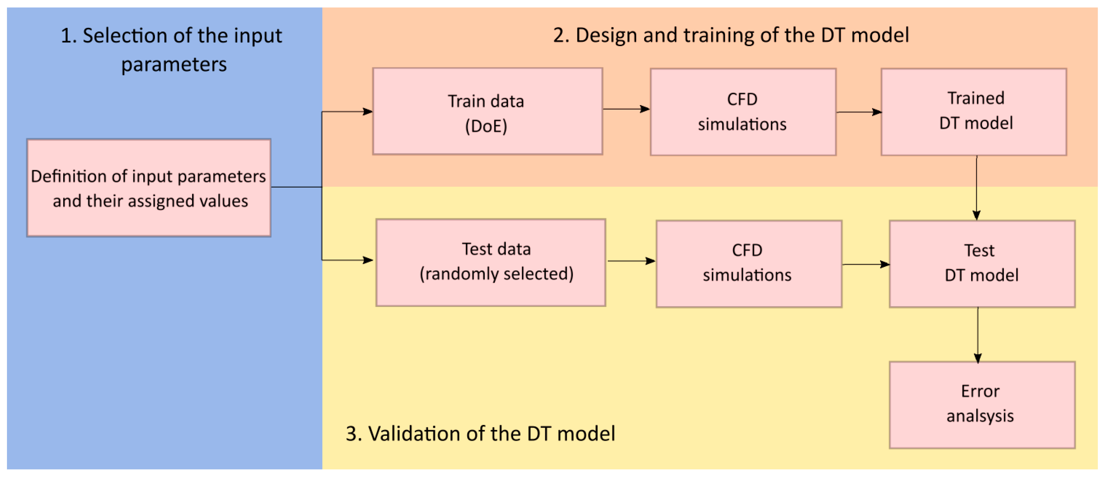
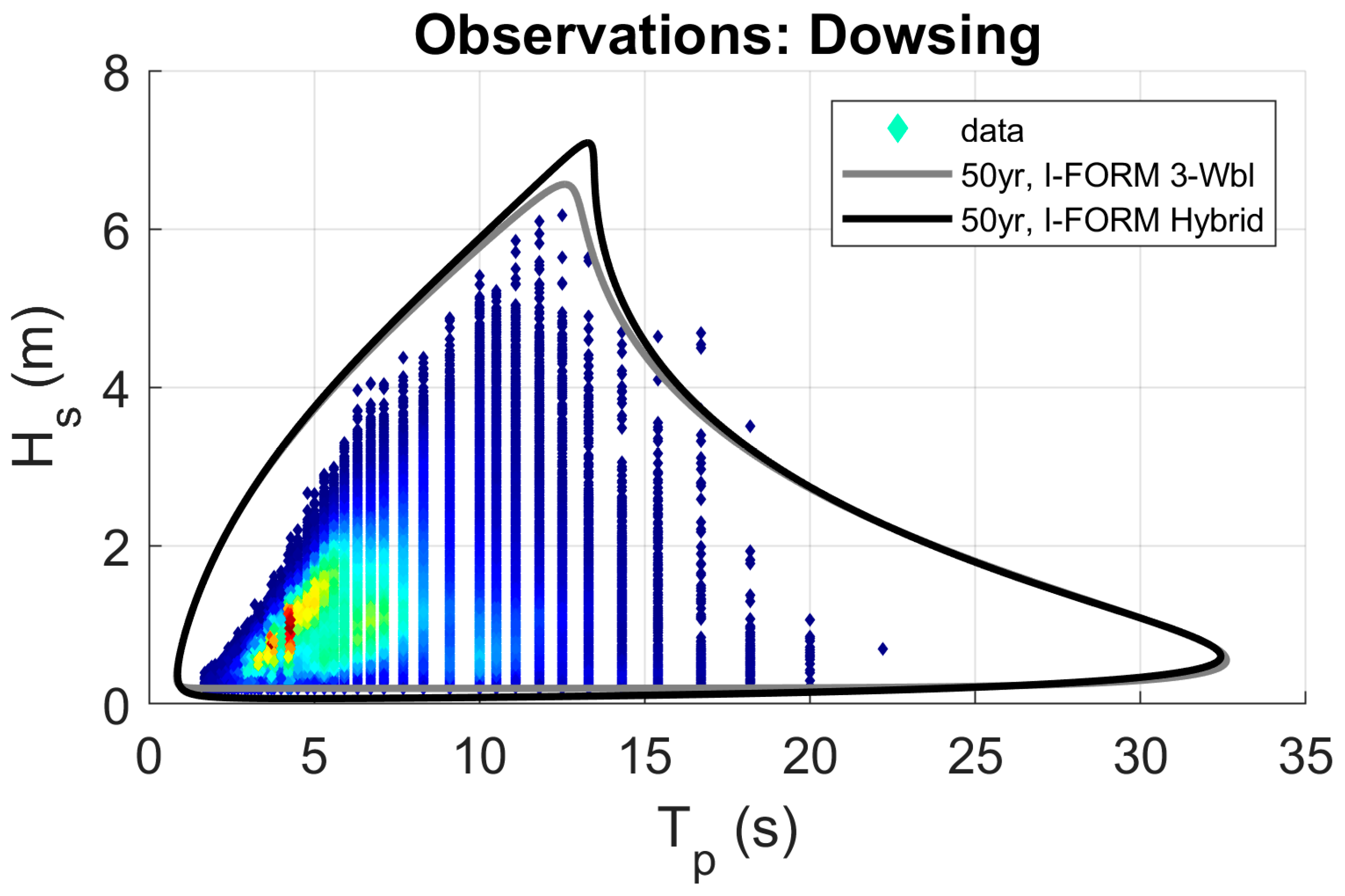
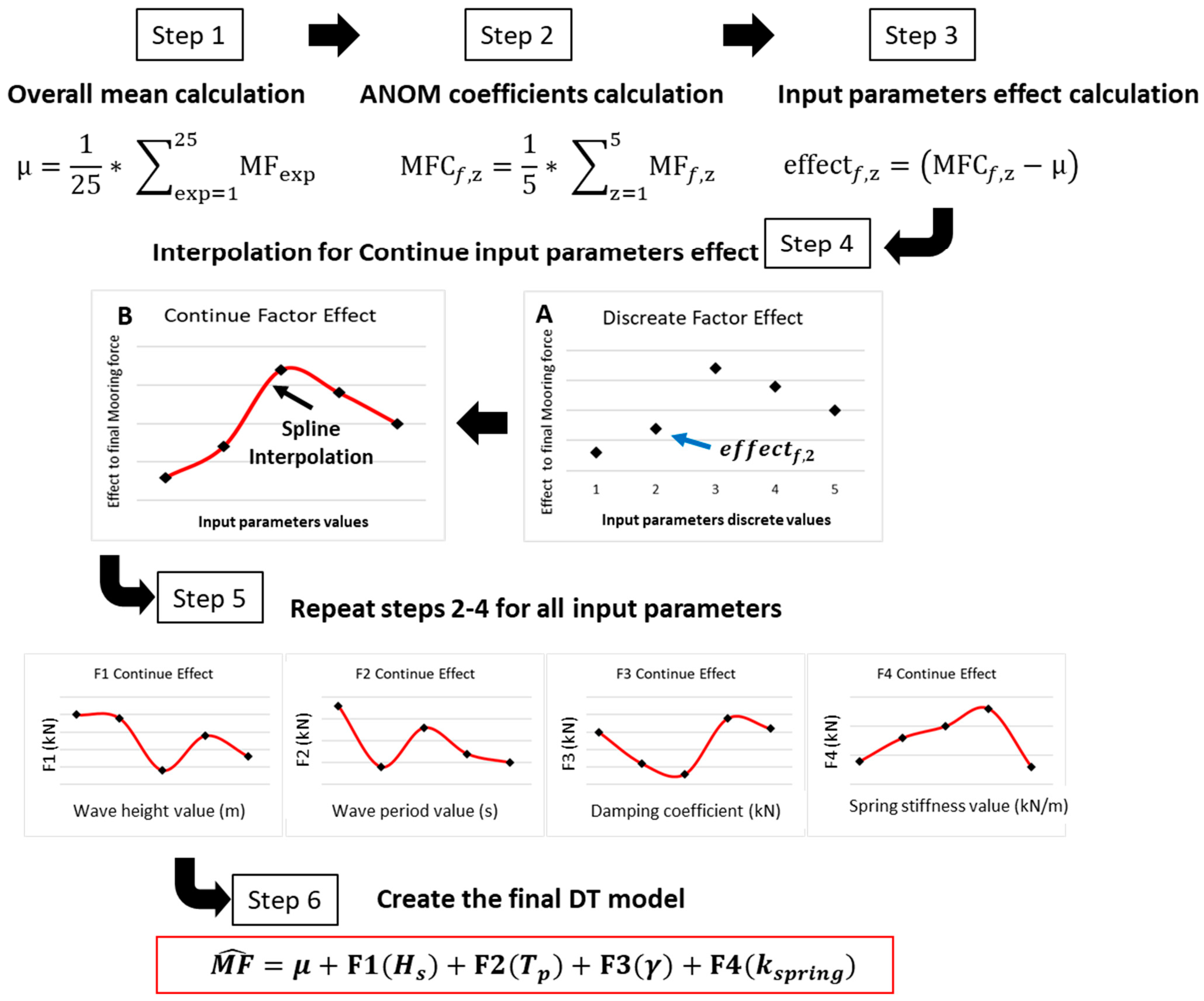
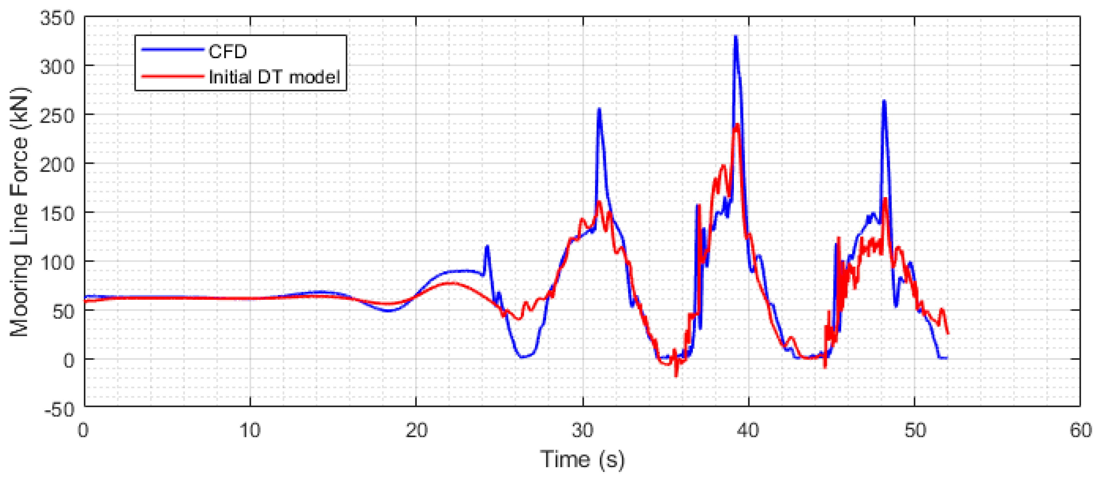
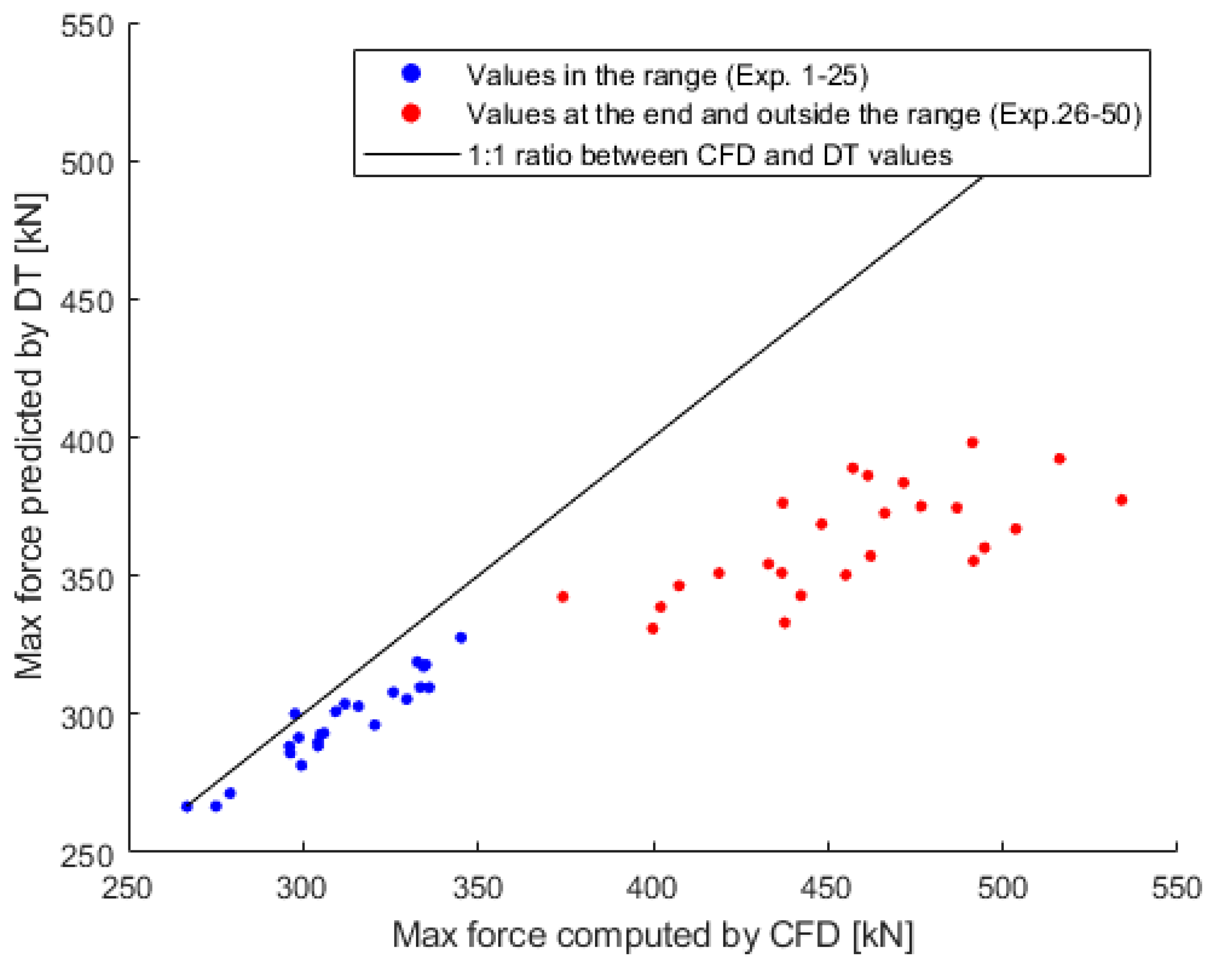
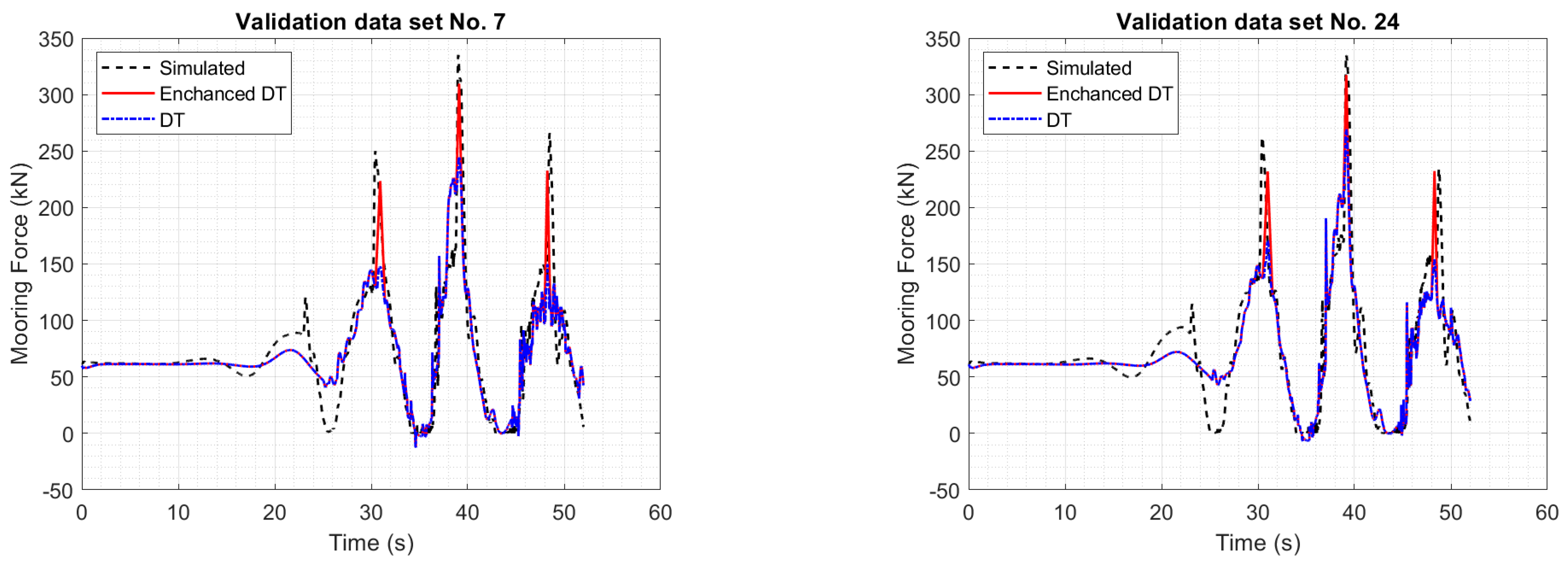
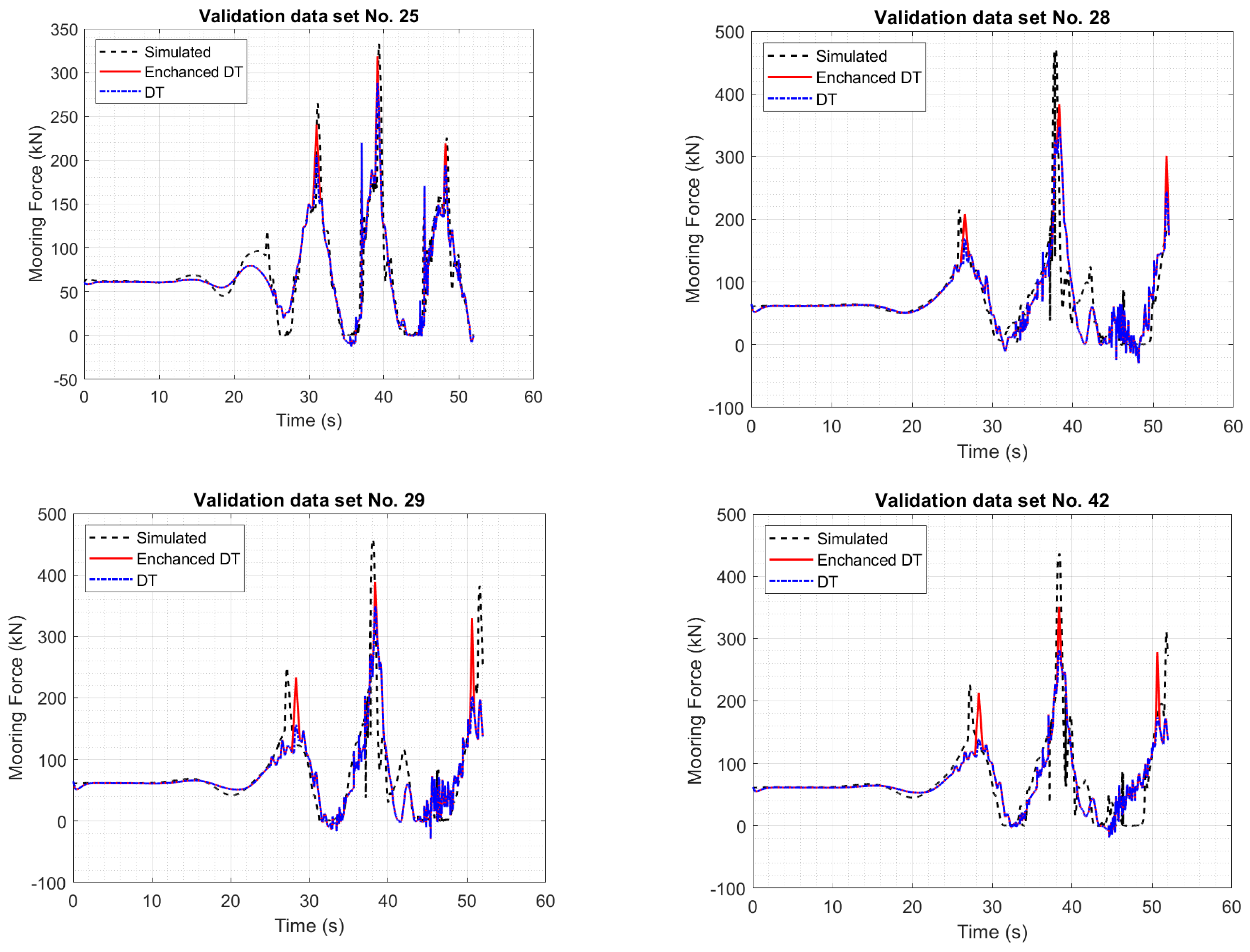
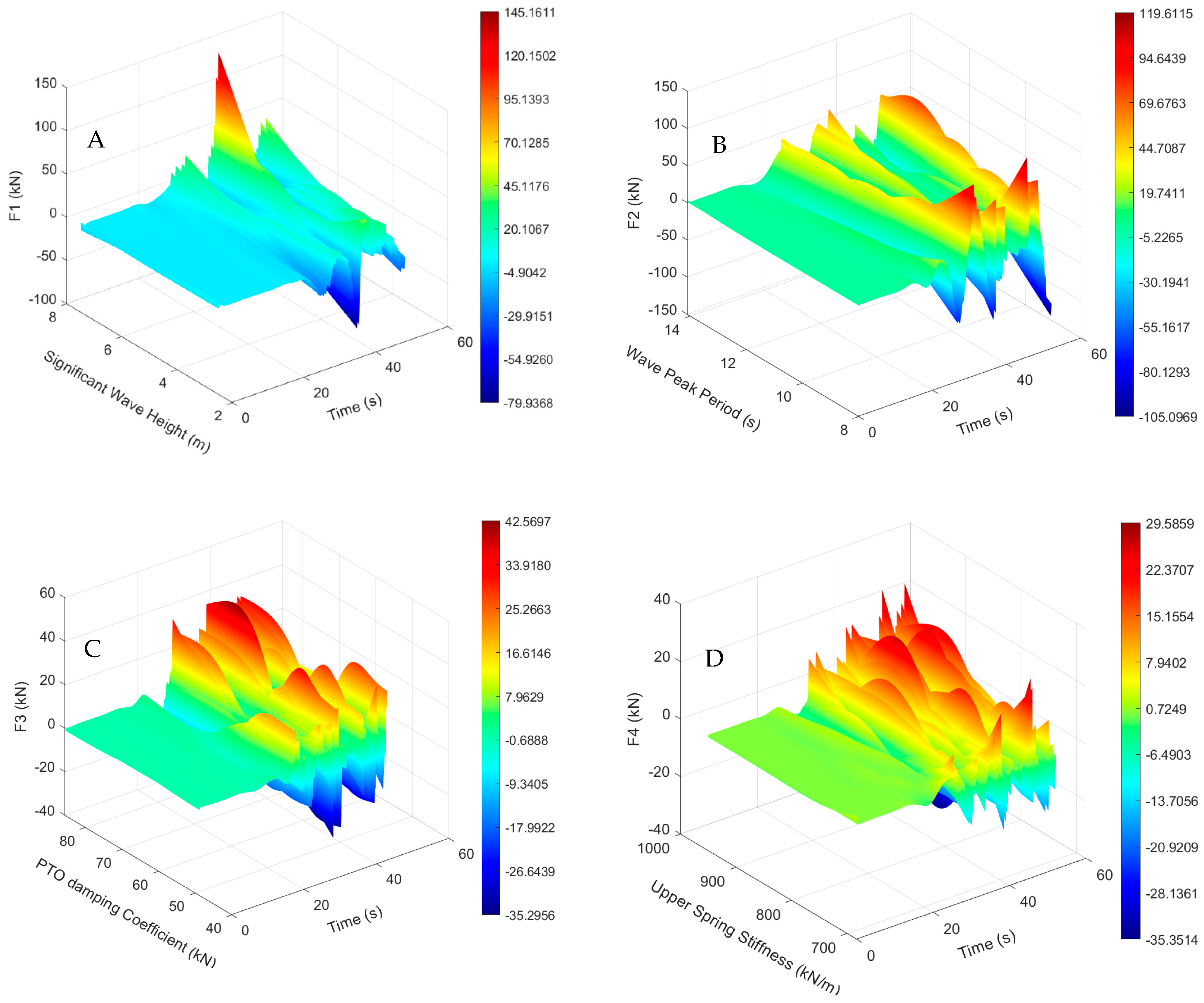
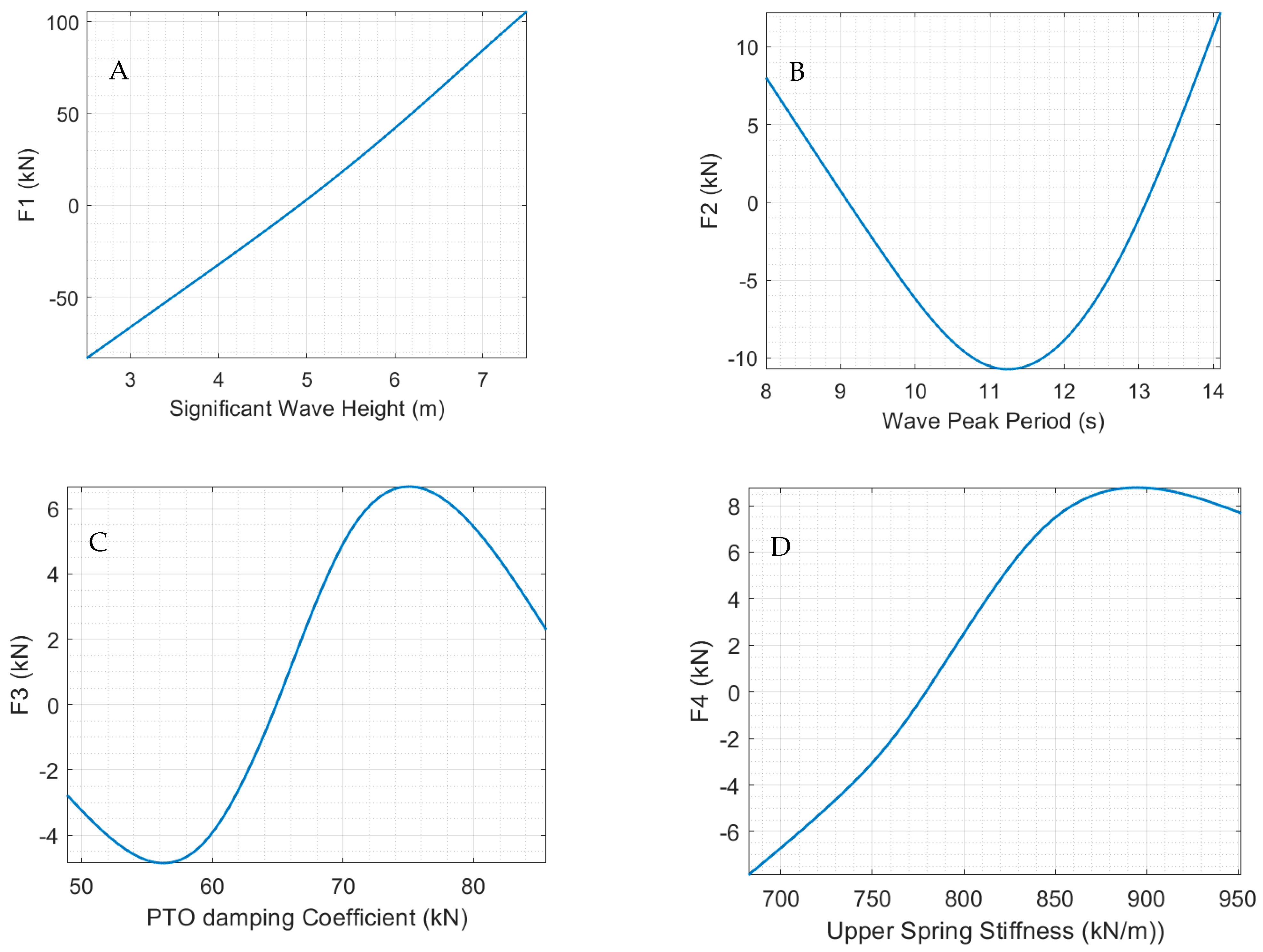