Analysis and Mitigation of Harmonic Resonances in Multi–Parallel Grid–Connected Inverters: A Review

Abstract

With the move towards decarbonization of the energy system and increased use of renewable generation, the number of power electronics converter interfaced resources connecting to the grid is growing. These power electronics converters have fast dynamics determined by control algorithms, which leads to significant changes in the dynamics and impedance characteristics of the power system. Based on practical experience, concerns have grown about interactions between converters and between converters and the grid which can give rise to instability in a system with multiple grid–connected inverters operating in parallel. This paper reviews the recent work related to the understanding, modeling and mitigation of such interactions. The basic concepts which underpin the interactions are explained and discussed from an impedance stability perspective. The concepts are illustrated by means of an example case of multiple inverters operating in a low voltage distribution system. In recent years, several approaches have been proposed to prevent or mitigate the effects of these interactions. The mitigation approaches proposed in the most recent works are categorized and comprehensively reviewed.

1. Introduction

Climate change is one of the century’s most pressing issues, and consequently there is a drive to reduce greenhouse gas emissions in an effort to limit global average temperature increases [1,2]. Among the important mitigation efforts being pursued, considerable resources are being dedicated to decarbonization of the electrical energy system. As a result, there continues to be an exponential increase in the use of distributed energy resources (DERs), such as solar photovoltaic (PV) and wind power [3]. In addition, decarbonization of the heating and transport sectors is leading to increased use of electric vehicles (EV) and heat pumps. DER, EVs and loads such as heat pumps are typically connected to the grid through a power–electronics–based voltage source inverter (VSI) or converter. Such inverter–based resources (IBR) are therefore, quickly becoming the dominant type of device in today’s power system [4], interfacing generation, storage and loads. This gives rise to the situation, particularly in the distribution system, whereby multiple IBRs are connected close to each other, which has raised concerns about the possibility of unwanted interactions between the inverters and between the inverters and the grid [5]. These interactions can manifest as oscillations in the grid current, which can lead to power quality problems and unexpected operation or shutdown of equipment.

Although traditionally individual inverters should be designed to work stably when grid connected (often referred to as internal stability), the parallel operation of many inverters raises the likelihood of new stability difficulties (often referred to as external stability). Some of the first studies which investigated these issues, see [6], were motivated by observations that networks with high penetration of PV inverters had power quality problems which exceeded standards and sometimes resulted in inverters switching off unexpectedly. Interactions were identified as being due to parallel resonances among the parallel inverters and series resonance between the parallel inverters and the grid. Recently, other instances of instability events have been observed from field experiences [7,8].

Most modern grid–connected inverters are equipped with an inductor–capacitor–inductor (LCL) filter to dampen the characteristic harmonics that are generated by the pulse width modulation (PWM) technique. The impact of the inverter LCL filter resonant frequency on the internal stability of the single grid–connected inverter has been a major concern, and various damping solutions to mitigate this have received considerable research attention. These techniques have received good reviews in previous works [9,10,11,12]. However, it is important to note that the resonance characteristics of the multi–parallel inverter system are distinct from the well–known resonance of the single VSI with an LCL filter. In previous reviews such as [13], LCL filter design and damping techniques for internal stability and modeling methods for external stability have been comprehensively reviewed; however, the treatment of interactions in multi–parallel inverter systems has been very brief.

In recent years, the concepts and causes underlying the interactions between multiple inverters have been investigated and refined. The basic cause is the existence of resonance frequencies which may be excited by harmonics present in the grid or in the inverters themselves. The existence of these resonant frequencies may also give rise to harmonic instability in the inverters. The interactions can be categorized as [14] being due to changes in the inverter’s own output current (referred to as internal or self resonance), which can be due to changes in the output current of other parallel connected inverters (referred to as interactive or parallel resonance) or changes in the grid voltage (referred to as series resonance).

As distinct from previous reviews, the focus of this review is on the resonances and interactions that may appear in a multiparallel grid–connected inverter system and their associated mitigation techniques. The review has a main focus on single phase distribution systems, as these systems are seeing the largest penetration of closely located DER. The underlying causes and many of the mitigation techniques reviewed are also relevant to three phase systems at the distribution and transmission levels. This study provides a review and explanation of the causes of interactions in multi–parallel inverter systems in Section 2. The various interactions are illustrated though the use of an example system in Section 3. Section 4 reviews the approaches which have been developed to attenuate the various resonances. Finally, Section 5 brings this paper to a close by discussing future work.

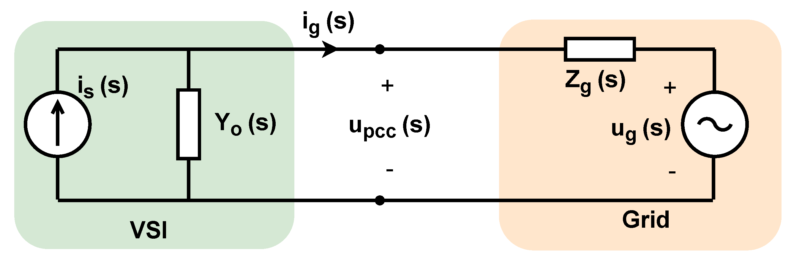
2. Stability of the Grid Connected VSI

Typically, stability issues have been investigated using one of two approaches: the state–space method in the time domain or the impedance–based method in the frequency domain [15,16]. In the state-space method, the stability assessment relies on the determination of the system’s eigenvalues. While this approach can accurately pinpoint the causes of system instability, it necessitates a full description of the system parameters. This makes it challenging to employ in a practical system, since all of those characteristics may not be well known and a rebuilding of the state space model is required if the operating point changes.

The impedance/admittance-based stability approach does not necessitate a complete description of all inverter control loops (known as “white box” model) because the VSI’s stability can be assessed based on its terminal characteristics [17]. Using the impedance–based stability technique, the VSI can be represented by its corresponding Norton’s equivalent circuit [18], and the grid it connects to as a voltage source in series with an impedance, as shown in Figure 1.

Considering the model in Figure 1, the current injected into the grid can be calculated based on the expression in (1):

$$i_g\left(s\right)=\{i_s\left(s\right)-u_g\left(s\right)·Y_o\left(s\right)\}·\frac{1}{1+\frac{Y_o\left(s\right)}{Y_g\left(s\right)}}$$

(1)

where $Y_g\left(s\right)=\frac{1}{Z_g\left(s\right)}$

Noting that the current $i_s\left(s\right)$ is the controlled current output of the inverter, then we can say that $i_s\left(s\right)=G_c\left(s\right)·i_g^{*}\left(s\right)$, where $G_c\left(s\right)$ is the closed loop transfer function of the reference current $i_g^{*}\left(s\right)$ to the output grid current. The expression for the grid current can then be written as:

$$i_g\left(s\right)=\{G_c\left(s\right)·i_g^{*}\left(s\right)-u_g\left(s\right)·Y_o\left(s\right)\}·\frac{1}{1+\frac{Y_o\left(s\right)}{Y_g\left(s\right)}}$$

(2)

It is worth noting that the expression of the injected grid current in (2) has two parts: the first term on the right–hand side represents the influence of the inverter’s closed loop current controller transfer function, and the second term represents the impact of the grid voltage. Internal stability of the converter refers to the stability of $G_c\left(s\right)$ [5,19]. External stability refers to the stability of the converter–grid system and depends on the stability of the minor loop $\frac{1}{1+\frac{Y_o\left(s\right)}{Y_g\left(s\right)}}$ [20]. According to [21], and assuming that the converter is internally stable, the grid–connected VSI system is externally stable if one of the following conditions is satisfied:

• $Y_g\left(s\right)$ = ∞, i.e., $Z_g\left(s\right)$ = 0.
• The ratio of $\frac{Y_o\left(s\right)}{Y_g\left(s\right)}$ satisfies the Nyquist stability criterion.

Since a null grid impedance is not a practical scenario, the VSI–grid system’s stability is largely determined by both the VSI output admittance $Y_o$ and the grid impedance $Z_g$. Grid impedance $Z_g$ will be different at different points in the grid and is typically not constant, since it varies over time due to the connection and disconnection of loads with varying characteristics, and grid faults that might affect the grid configuration. As a result, the VSI output admittance $Y_o$ should be tailored to ensure the stability of the VSI–grid system considering a wide range of grid impedance variations.

The output admittance of the VSI is frequency dependent, since it is affected by various control loops which are effective over different frequency ranges [22]. For instance, slower control loops, such as the dc link/power control loop, in addition to the phase locked loop (PLL), shape the low frequency behavior of the output admittance. The current control loop, on the other hand, has a larger bandwidth and hence dominates the medium–to–high frequency area of the output admittance. The control delay and the filter parameters [23] tend to determine the high frequency characteristic of the VSI output admittance. It is worth noting that the sampling frequency or Nyquist frequency presents an upper limit to the validity of the impedance model for the active part of the impedance, which is related to the controllers. However, the controller bandwidth tends to be lower than the Nyquist frequency, so that the contribution of the controllers to the impedance at frequencies close to or above the Nyquist frequency is negligible. At these frequencies, the passive part of the impedance due to the physical inductance, capacitance and resistance in the system dominates. Therefore, the impedance model may still be valid, although special attention would need to be given to accurately model the behaviors of these passive elements at high frequency.

The frequency response, or Bode plot, of both the VSI’s and the grid’s admittances, can be used to assess the VSI–grid system’s stability. When assessing the impedance stability of the VSI–grid system, two crucial points in the Bode plots of both admittances should be examined [24]:

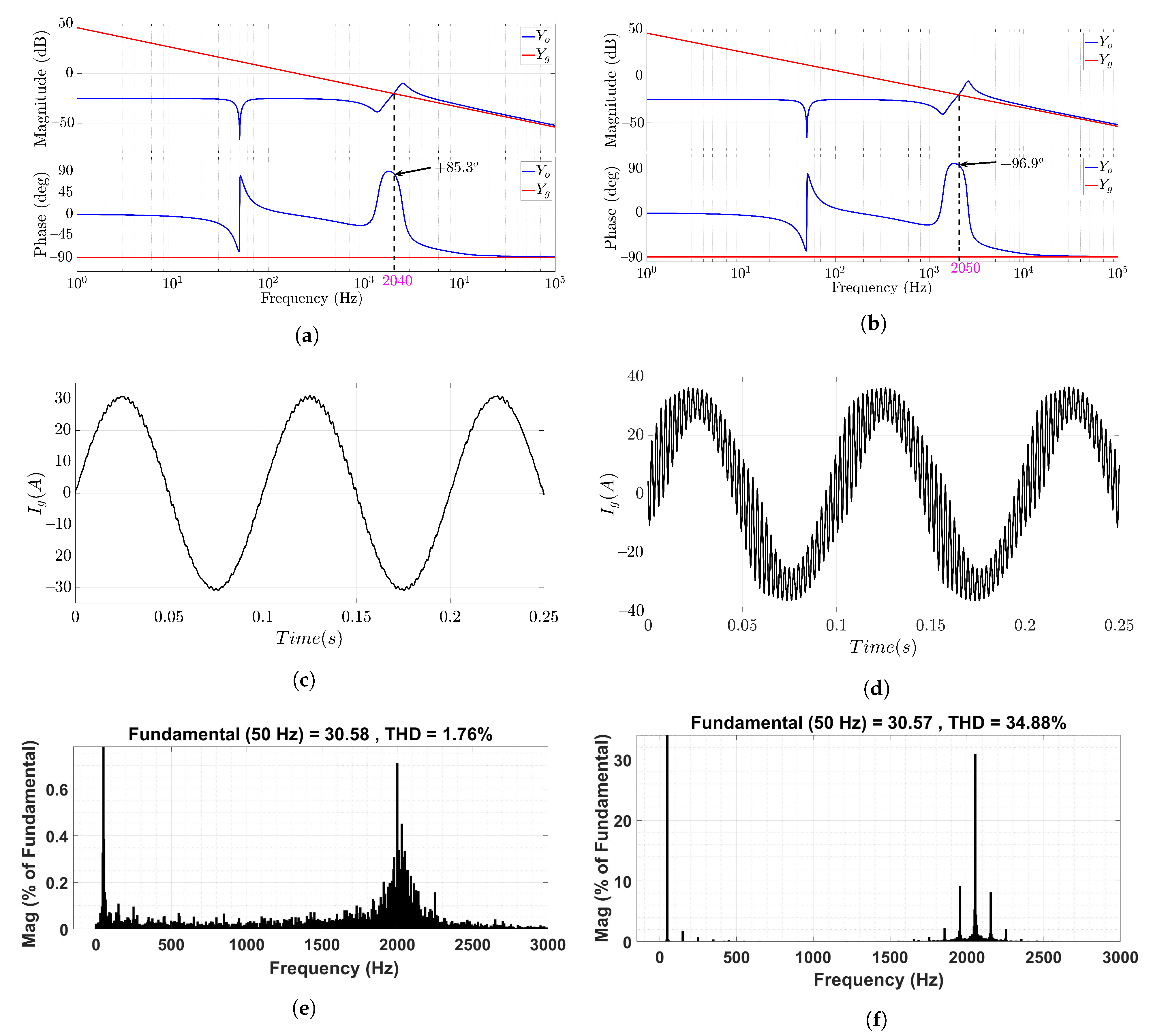
• The intersection points of the magnitude curves for the inverter output admittance $Y_o$ and the grid admittance $Y_g$, which represent the zero–dB crossing points of their ratio.
• The phase margin ${\varphi }_{PM}$ at the intersection point of $Y_o$ and $Y_g$, which can be calculated as:

  $${\varphi }_{PM}=180-[{\varphi }_{Y_o}-{\varphi }_{Y_g}]$$

  (3)

  where ${\varphi }_{Y_o}$ and ${\varphi }_{Y_g}$ are the phase angle of the inverter output admittance and the grid admittance, respectively. A positive phase margin angle ensures the VSI–grid system’s stability [25].

Assuming a passive grid impedance, the stability of the VSI–grid system can be guaranteed if the real part of the output admittance (also known as the conductance) is nonnegative for all frequencies. This essentially guarantees that its angle is always $\pm 90$°, and the output admittance of the grid–connected inverter can be regarded as being a passive admittance. Conversely, if an intersection point of $Y_o$ and $Y_g$ occurs within a nonpassive region where the VSI output admittance has a negative real part, the VSI–grid system may potentially be unstable. It can be the case that the VSI output admittance has a negative resistance behavior only in specific frequency ranges [26], and for example, the study in [27] established an admittance model that decomposes the VSI output admittance into active and passive admittance components. The current controller and time delay influence the former, and the filter parameters determine the latter. Overall, the VSI output admittance can be guaranteed to be passive if two conditions are met [28]:

• The admittance itself has no right half-plane poles, which implies that the VSI is internally stable at the point of common coupling (PCC), i.e., stable when connected to an ideal zero impedance grid.
• The admittance has a real part which is nonnegative, i.e., $Re\{Y_o\left(j\omega \right)$$⩾0$, $\forall \omega$}, which indicates that the phase of $Y_o\left(j\omega \right)$ is within [−90°, 90°].

To minimize the negative-real–part of the inverter output admittance, some design recommendations are discussed in [29] and can be summarized as follows:

• A smaller total time delay (computation-plus–PWM, time delay) associated with sampling and PWM can improve the passivity of the output admittance.
• A lower bandwidth of the outer loops, such as the dc link/power control loop and the PLL.
• Using the stationary reference frame ($\alpha \beta$ frame) in the current controller helps restrict the PLL influence because the negative–real–part region due to the PLL effect extends if the current controller employs a $dq$-frame.

Further parameters that influence the passivity of inverter output admittance, such as the use of multisampling, the use of capacitor current feedback active damping and various PLLs, are assessed in [30]. In the multisampling technique, the sampling and modulation signals are updated numerous times in a switching cycle, $T_{sm}=T_{sw}/N$, where $T_{sw}$ is the switching time of the VSI and N is the coefficient of multisampling. This is advantageous in terms of decreasing the control delay induced by regular sampling and widening the system’s control bandwidth [31,32]. The study in [30] revealed that the multisampling coefficient and capacitor current feedback active damping dominate the high–frequency band. For high power and low switching frequency applications, a higher multisampling coefficient is recommended to improve the passivity of the inverter output admittance. Furthermore, a large value of the capacitor current feedback active damping coefficient is advisable to improve the passivity of the output admittance in the high–frequency band when the VSI is connected to an inductive grid impedance. However, if the grid impedance has a capacitive behavior, then the system stability could still be an issue. The influence of the PLL, on the other hand, is only seen in the low–frequency region of the inverter output admittance. The non-passive portion of the inverter output admittance in the low frequency region often narrows as the PLL bandwidth shrinks.

Clearly, in the case where the phase margin associated with the admittance ratio is greater than zero, the injected grid current can be guaranteed to be stable. However, if the phase margin is positive but too small, then the power quality of the grid current may be compromised, as transients can cause damped oscillations that affect overall total harmonic distortion (THD). The grid current’s stability and power quality are always closely related [33,34]. As discussed above, the integration of the VSI in a grid with non–negligible impedance can degrade the VSI’s external stability [20] due to the occurrence of a critical resonance frequency at the intersection frequency of $Y_o$ and $Y_g$. When the phase margin angle is positive at this frequency, the resulting resonant component of current in the grid may be stable, but the value of the phase margin influences the quality of the grid current. A large phase angle, implying sufficient damping, is required to suppress this resonant component to the lowest value possible, so that the injected grid current’s THD level is adequate. Therefore, not every stable grid current will have a sufficient power quality metric; however, improving power quality suggests a more stable system.

In general, the grid current oscillations caused by the impedance interactions may be transient or steady-state oscillations. Transient oscillations are oscillations that last for a short period of time and may be triggered by a sudden change in the current reference or load change, or voltage sags and swells in a few fundamental cycles of the grid voltage [14]. A sufficiently large phase margin at the impedance intersection point is required to quickly suppress such transient oscillations. Steady–state oscillations, on the other hand, are oscillations that are sustained and are not naturally dampened. The steady–state background harmonics and harmonic resonances that emerge due to interactions in the VSI-grid system cause these oscillations [35].

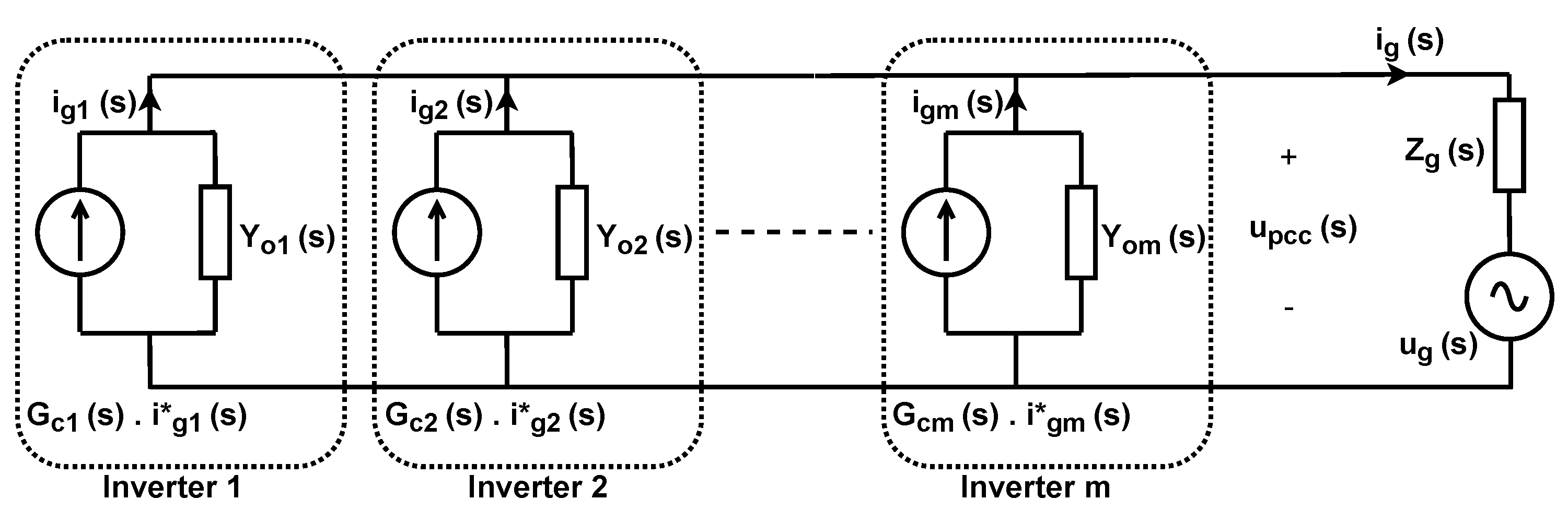
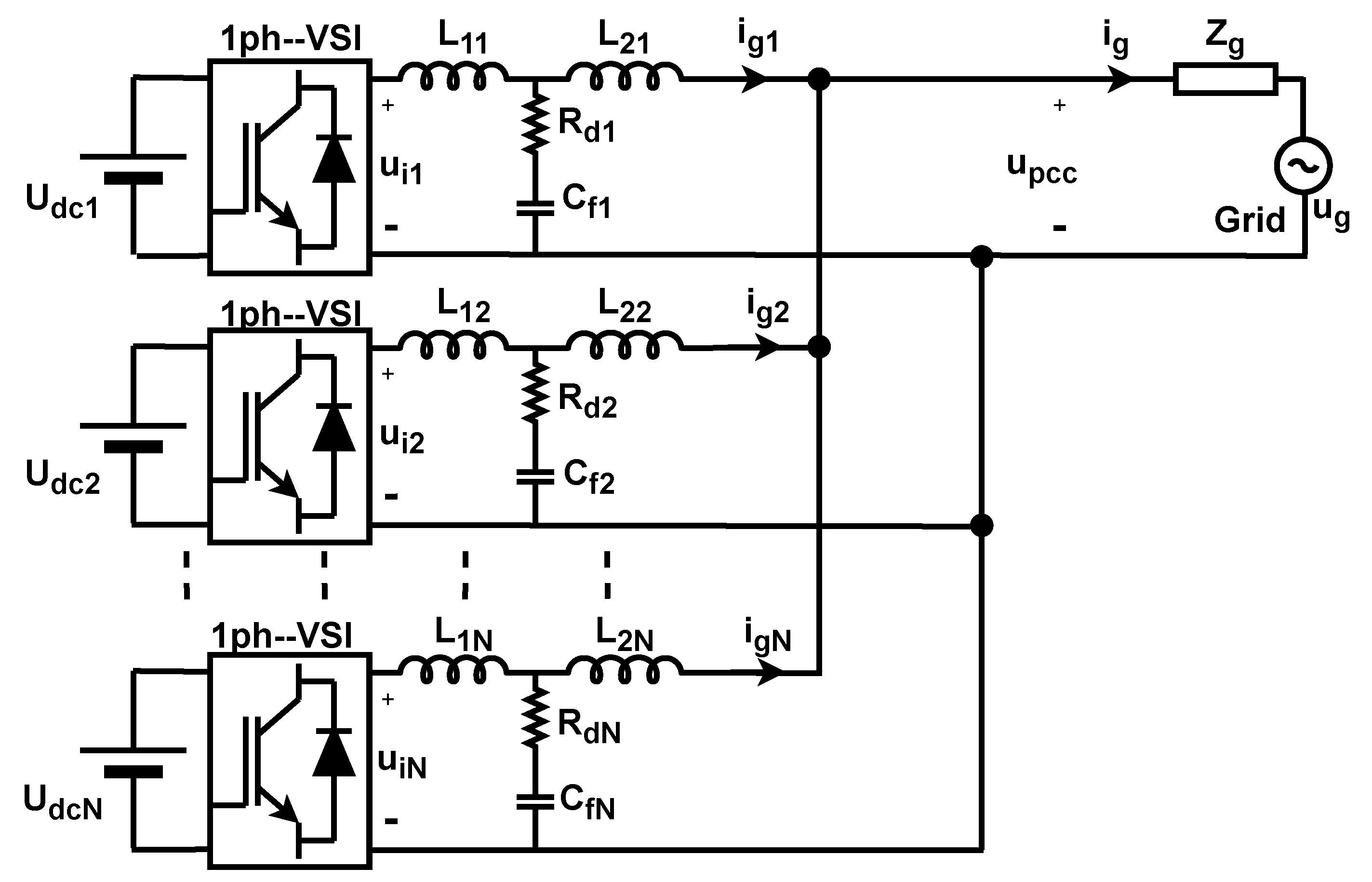
2.1. Multi–Parallel Inverter–Grid System

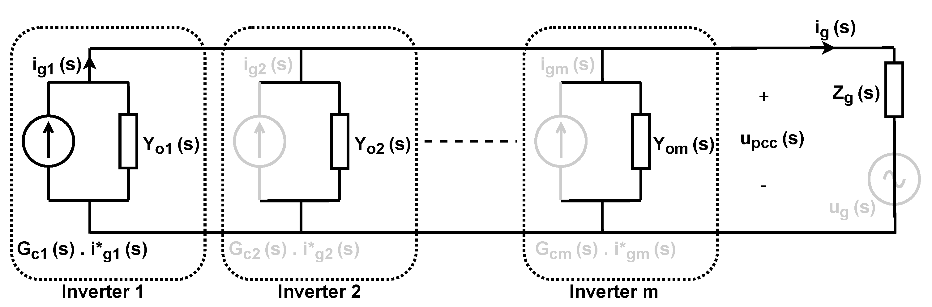
The model of Figure 1 can be extended to the case of multi–parallel grid–connected inverters, as shown in Figure 2. In this case, and with reference to superposition, the injected current of the target inverter—for example, see $i_{g1}\left(s\right)$ in Figure 2—can be divided into three main components, which are referred to as the main current, the interactive current and the common current [36,37]. The main current is due to the output of the inverter itself. The interactive current is the portion of the output current of the other parallel inverters which flows though the output impedance of the target inverter. Essentially, this is a current that flows or circulates among the inverters, and is also sometimes referred to the circulating current. The common current is the portion of current due to the grid voltage acting on the inverter output impedance.

In comparison to a single inverter, the impedance interactions of parallel inverters are therefore more intricate. The resonance of the single VSI can be caused by the external interaction of the single inverter with a passive grid. In contrast, the resonance of the parallel VSIs is more challenging, as the VSI interacts externally with what can be viewed as an active grid impedance composed of the dynamics of the other parallel inverters, as shown in Figure 2.

2.2. Main Current

As previously stated, the main current is the contribution made to the output current of the inverter from its own current source. Using superposition, it can be considered to be the current $i_{g1}\left(s\right)$ which flows when all of the other parallel inverter current sources and the grid voltage is set to zero, as shown in Figure 3.

For the sake of illustration, we will assume that all inverters are identical. The source current of inverter i will divide between its own output admittance and the output admittances of the parallel inverters and the grid admittance. Considering this current division, the transfer function relating the main current for inverter i to its reference current, in a system with n identical inverters in parallel, can be derived as in Equation (4) [38].

$$\frac{i_{g,i}\left(s\right)}{i_{g,i}^{*}\left(s\right)}=G_{ii}\left(s\right)=G_{c,i}\left(s\right)·\{1-\frac{Y_o\left(s\right)}{n·Y_o\left(s\right)+Y_g\left(s\right)}\},wherei=1,2,3,\dots$$

(4)

To better illustrate the relationship with the external impedance stability conditions discussed earlier for the single inverter–grid case, Equation (4) can be rearranged as shown in (5):

$$G_{ii}\left(s\right)=G_{c,i}\left(s\right)·\{1-\frac{Y_o\left(s\right)}{n·Y_o\left(s\right)+Y_g\left(s\right)}\}=G_{c,i}\left(s\right)·\left\{\frac{1}{1+\frac{Y_o\left(s\right)}{(n-1)·Y_o\left(s\right)+Y_g\left(s\right)}}\right\},wheren>1$$

(5)

The term $\frac{1}{1+\frac{Y_o\left(s\right)}{(n-1)·Y_o\left(s\right)+Y_g\left(s\right)}}$ in (5) represents a closed–loop transfer function of a negative feedback control system, where the forward gain is unity and the feedback gain is $\frac{Y_o\left(s\right)}{(n-1)·Y_o\left(s\right)+Y_g\left(s\right)}$; that is, the ratio of the source output admittance of a target inverter to the load admittance of the other parallel inverters and the grid admittance. Therefore, the external stability of the main current of inverter i is guaranteed only if $\frac{Y_o\left(s\right)}{(n-1)·Y_o\left(s\right)+Y_g\left(s\right)}$ satisfies the Nyquist stability criterion [38].

2.3. Interactive Current

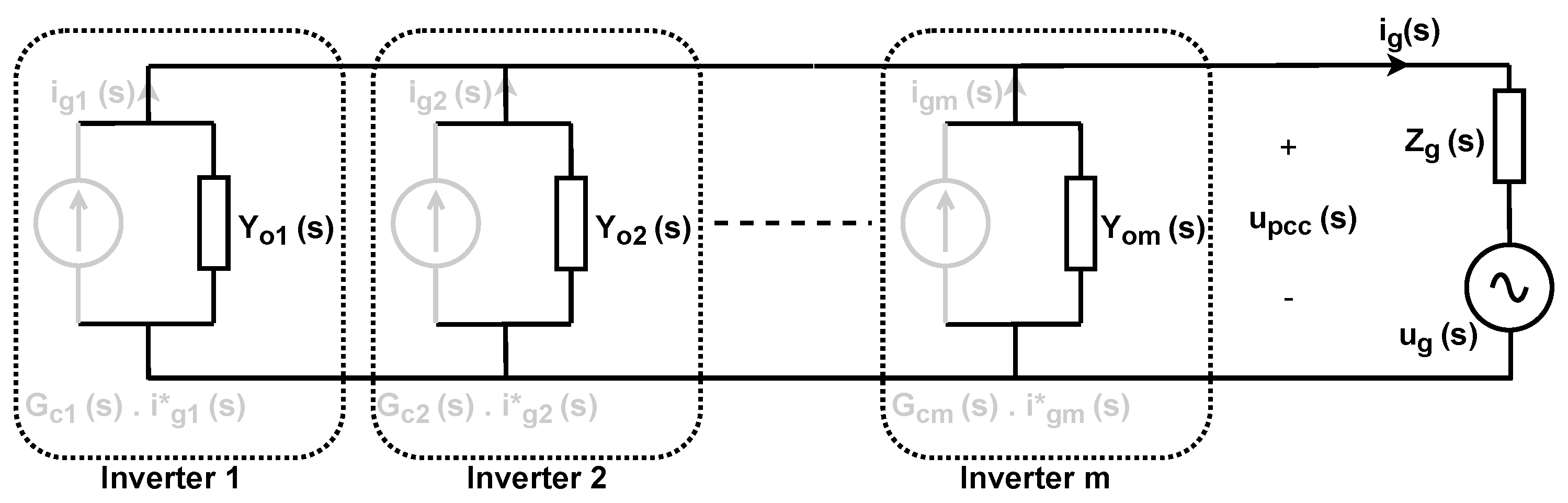
The influence of the output current of the other inverters on the grid side current of the examined inverter is represented by the interactive current component. This interactive current has a contribution from each of the other parallel connected inverters. The circuit shown in Figure 4 can be used to show the contribution from one such current source, j, to the interactive current of the target inverter, i.

Again, using current division, the transfer function that relates the interactive current of the target inverter, i, to the reference current of the other inverter output voltage, j, can be derived as:

$$\frac{i_{g,i}\left(s\right)}{i_{g,j}^{*}\left(s\right)}=G_{P_{i,j}}\left(s\right)=G_{c,j}\left(s\right)·\left\{\frac{Y_o\left(s\right)}{n·Y_o\left(s\right)+Y_g\left(s\right)}\right\}=G_{c,j}\left(s\right)·\left\{\frac{1}{1+\frac{(n-1)·Y_o\left(s\right)+Y_g\left(s\right)}{Y_o\left(s\right)}}\right\},wherei\ne j$$

(6)

A similar conclusion can be drawn regarding the stability of this interactive current component as in the case of the main current. Assuming inverter j is internally stable, then the stability of the interactive component of current depends on the stability of the admittance ratio $\frac{(n-1)·Y_o\left(s\right)+Y_g\left(s\right)}{Y_o\left(s\right)}$.

2.4. Common Current

The parallel inverters’ integration in the utility grid gives rise to a component of current caused by the grid voltage being applied across the output admittance of all of the parallel inverters. The equivalent admittance model in Figure 5 can be used to assess this current. The impact of the utility grid voltage on the injected current from the target inverter, i, is given by the transfer function in (7) (which is equivalent to an admittance):

$$\frac{i_{g,i}\left(s\right)}{u_g\left(s\right)}=G_{s,i}\left(s\right)=Y_g\left(s\right)·\left\{\frac{Y_o\left(s\right)}{n·Y_o\left(s\right)+Y_g\left(s\right)}\right\}=Y_g\left(s\right)·\left\{\frac{1}{1+\frac{(n-1)·Y_o\left(s\right)+Y_g\left(s\right)}{Y_o\left(s\right)}}\right\},wherei=1,2,3,\dots ..$$

(7)

Again, the impedance stability of the common current can be seen to depend on the impedance ratio $\frac{(n-1)·Y_o\left(s\right)+Y_g\left(s\right)}{Y_o\left(s\right)}$.

To more clearly illustrate all of the above concepts in the context of a typical single phase, multi–paralleled, grid–connected VSI system, the next section presents an illustrative example.

3. Example of Resonances in a Multi–Parallel Grid–Connected Inverter System

The configuration of the example of multi–parallel grid–connected VSI system is shown in Figure 6, where each VSI is provided with an LCL filter, which is widely adopted in the modern grid-connected inverters. The parallel inverters are connected to the grid, which is modeled as a voltage source in series with a lumped grid impedance $Z_g$ at the point of common coupling (PCC).

3.1. Model of Single VSI

The grid-connected VSI is composed of two main circuits, the power circuit and the control circuit, as shown in Figure 7. The power circuit consists of a dc–ac inverter coupled to an LCL filter to suppress switching harmonics created by the pulse width modulation (PWM) circuit, where $L_1$ and $L_2$ are the inverter–side and grid–side inductors, respectively. The filter capacitor is $C_f$, and the passive damping resistor for the intrinsic LCL filter resonance peak is $R_d$. To produce the appropriate inverter output voltage, $u_i$, the inverter is powered by a fixed dc voltage, $U_{dc}$, whose magnitude must always be greater than the amplitude of the ac voltage.

The phase locked loop (PLL) works to synchronize the generated current to the grid voltage in the second portion of the control diagram of the grid–side current–controlled VSI. This PLL is based on the second order generalized integrator (SOGI), which has been shown to be effective [39]. Meanwhile, the current $I_m$ is the peak value of the reference current that represents the VSI’s operational point and is created by the outer loop control, which can be either the power control loop or the dc–link voltage loop. The grid current is controlled in the stationary reference frame ($\alpha \beta$ frame) by a proportional–resonance (PR) controller, which has been shown to have a more robust performance [40].

To apply the impedance-based stability approach, a linearized, small signal model of the grid–connected VSI should be developed.

3.2. Small-Signal Model

Figure 8 shows the control block diagram of the VSI with grid–side current control.

$G_{pr}\left(s\right)$ is the transfer function of the PR current controller which is expressed in (8), where $k_p$ is the proportional gain and $k_r$ is the resonant integral gain. To avoid the infinite gain at the nominal grid frequency ${\omega }_g$, a proper selection of cut-off frequency, ${\omega }_c$ is considered, where (${\omega }_c\ll {\omega }_g$) [41].

$$G_{pr}\left(s\right)=k_p+k_r\frac{2{\omega }_{c}s}{s^2+2{\omega }_{c}s+{\omega }_g^2}$$

(8)

The grid current is digitally controlled, so the computation and PWM delays of the digital controller are represented by the delay transfer function $G_{de}\left(s\right)$ in (9), where $T_s$ is the sampling period [42].

$$G_{de}\left(s\right)=e^{-1.5s{T}_s}$$

(9)

The dissipation that occurs in resistances of the inductors of the LCL filter is ignored to simplify the analysis, which also corresponds to the worst working conditions of the LCL filter. The equivalent transfer function of the filter capacitor branch $G_f\left(s\right)$ can be expressed in (10)

$$G_f\left(s\right)=\frac{s{C}_f}{1+s{C}_f{R}_d}$$

(10)

The VSI output admittance $Y_o$ can be found from the VSI’s small–signal model in Figure 8. By omitting the input reference current, the output admittance of the VSI can be derived as:

$$Y_o\left(s\right)=\frac{-i_g\left(s\right)}{u_{pcc}\left(s\right)}=\frac{1+L_1{G}_{f}s}{L_1{L}_2{G}_f{s}^2+(L_1+L_2)s+G_{pr}{G}_{de}}$$

(11)

The output current depends on the reference current, and the closed loop transfer function, $G_c\left(s\right)$, of the reference current $i_g^{*}\left(s\right)$ to the output grid current $i_g\left(s\right)$, can be derived as:

$$G_c\left(s\right)=\frac{i_g\left(s\right)}{i_g^{*}\left(s\right)}=\frac{T_m\left(s\right)}{1+T_m\left(s\right)}$$

(12)

where $T_m\left(s\right)$ is the loop gain of the current control loop and can be expressed as:

$$T_m\left(s\right)=G_{pr}\left(s\right)·G_{de}\left(s\right)·G_{LCL}=G_{pr}\left(s\right)·G_{de}\left(s\right)\frac{1}{L_1{L}_2{G}_f{s}^2+(L_1+L_2)s}$$

(13)

where $G_{LCL}$ is the transfer function of the LCL filter plant.

Given these derivations, an exemplary scenario is illustrated in order to shown the distinct resonances that may arise in the multi–parallel grid–connected inverter system. The rated data of the example VSIs that are employed in this study are listed in

Table 1. Rated data, LCL filter parameters, PR current controller gains of the identical grid–connected VSI and the grid impedance value.

Parameter	Symbol	Value
Rated Power	$P_o$	5 kW
DC link Voltage	$U_{dc}$	400 V
Grid voltage	$U_g$	230 V
Grid frequency	$f_g$	50 Hz
Switching frequency	$f_{sw}$	10 kHz
Sampling frequency	$f_s$	20 kHz
Inverter–side Inductor	$L_1$	2.6 mH
Grid–side Inductor	$L_2$	0.65 mH
Filter Capacitor	$C_f$	5 µf
Damping resistor	$R_d$	4.8 $\mathsf{\Omega }$
PR controller gains	$k_p,k_r$, ${\omega }_c$	18.35, 2017, 0.5
Grid impedance	$L_g$	0.8 mH

, where the filter parameters, the controller gains and the grid impedance are included.

3.3. Single Inverter Grid Interaction

If we first consider the connection of a single inverter to the grid; then the admittances of concern are the output admittance $Y_o$ of the single inverter and the grid admittance $Y_g$.

Two cases are illustrated in Figure 9 below, a case where the single inverter is externally stable with grid (Figure 9a,c,e) and an unstable situation (Figure 9b,d,f). Figure 9a illustrates that the intersection point in the magnitude plot of the output admittance $Y_o$ of a single inverter and the grid admittance $Y_g$ occurs at the frequency of 2040 Hz in the stable situation. At that frequency, the VSI–grid system’s phase margin angle, ${\varphi }_{PM}$, equals +4.5${}^{\circ }$. The VSI-grid system’s stability is therefore assured, as shown in Figure 9c. However, the resonance frequency dominates the harmonic spectrum of the injected grid current, as depicted in Figure 9e.

An unstable case can be achieved by, for example, slightly reducing the passive damping of the LCL resonance frequency (from 4.8 $\mathsf{\Omega }$ to 3.7 $\mathsf{\Omega }$). In this case, the grid–connected VSI is internally stable, but the nonpassive region of the VSI output impedance gets wider, causing an external instability problem. For the unstable case, the intersection point in the magnitude plot of the output admittance $Y_o$ of a single inverter and the grid admittance $Y_g$ occurs at the frequency of 2050 Hz, as depicted in Figure 9b. The VSI–grid system in this instance has a negative phase margin angle, ${\varphi }_{PM}$, of −6.9${}^{\circ }$, which foresees the injection of an unstable current into the grid. The simulation result provided in Figure 9d confirms this expectation. Additionally, as shown in Figure 9f, the harmonic spectrum of the injected grid current is dominated by that resonance frequency.

It is worth noting that in this example the converters’ Nyquist frequency is equal to the switching frequency and does not influence the validity of the impedance model. In the admittance model in Figure 9a,b, the harmonic resonance results from the inductive behavior of the grid impedance and the capacitive behavior of the VSI output impedance. The capacitive behavior of the output impedance occurs between the LCL filter’s anti-resonance peak and resonance peak. These two peaks depend on the resonance frequency of the LCL filter, which is typically chosen to be less than half the switching frequency and larger than 10 times the fundamental frequency. Therefore, the output impedance model of the VSI that includes the effect of the controllers is still valid at this critical resonance frequency.

Next, we consider the connection of n inverters in parallel to the grid and the characteristics of the three main components of resultant currents, i.e., the main current, the interactive current and the common current.

3.4. Main Current Resonance of the Inverter Itself

The frequency response of the main current transfer function ($G_{ii}$) is shown in Figure 10. These plots are generated by considering the system with n parallel identical inverters which have the parameters tabulated in Table 1, where the $Y_o\left(s\right)$ are obtained from (11). In Figure 10, there are two resonance peaks. One of them is fixed and depends on the VSI current controller and the filter parameters, and the other one moves lower in frequency as the number of parallel inverters increases [43]. According to (4), the fixed resonance peak is due to the closed loop current controller $G_{c,i}\left(s\right)$, and the movable resonance peak is due to the admittance ratio term $\left\{\frac{Y_o\left(s\right)}{n·Y_o\left(s\right)+Y_g\left(s\right)}\right\}$.

It is worth noticing that, as shown in Figure 10, the magnitude of $G_{11}\left(s\right)$ in the high frequency area increases with the number of paralleled inverters. This can be interpreted using Equation (4), which can be rearranged to analyze the high frequency behavior. In the high frequency region, the output admittance of the N-parallel inverters becomes larger than the grid admittance $|n·Y_o|\gg \left|Y_g\right|$. As a result, Equation (4) can be simplified further as in (14):

$$G_{ii}\left(s\right)\approx G_{c,i}\left(s\right)·\{1-\frac{1}{n}\}$$

(14)

From (14) it can be seen that as n increases, $G_{ii}$ will also increase.

The magnitude and frequency of the movable resonance peak decreases as the number of parallel inverters increases. This resonance arises from the intersection point of $Y_o$ and $(n·Y_o+Y_g)$, as indicated in (4). It will be shown later that as n increases, this intersection moves to a lower frequency and is more damped, hence the observed changes in frequency and magnitude of this resonance.

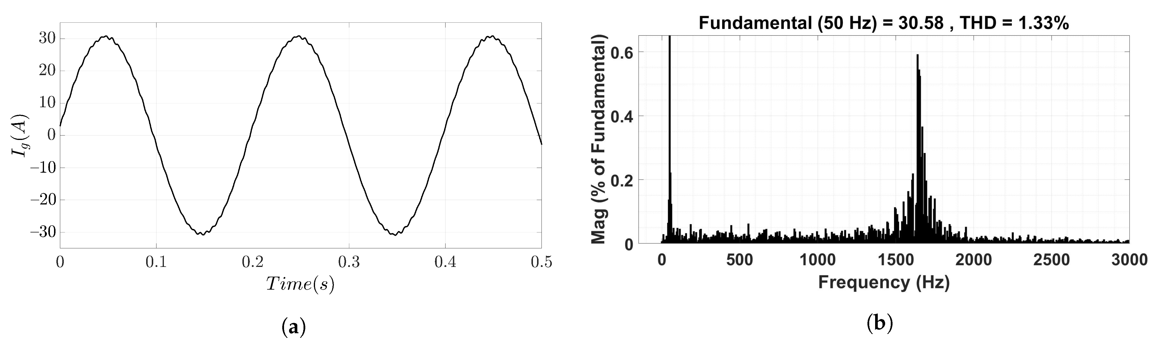
3.5. Interactive Current Resonance

The interactive current resonance transfer function, like the main current resonance’s, also has two resonance peaks, fixed and movable. The fixed peak is also determined by the filter parameters and the VSI current controller. The frequency of the fixed peak is similar to the main current resonance and is associated with the transfer function $G_c\left(s\right)$, since identical inverters are utilized. The movable resonance peak is associated with the admittance ratio term in (6), and because the frequency of the intersection of $Y_o\left(s\right)$ and $n·Y_o+Y_g$ decreases as the number of parallel inverters increases, the movable resonance peak moves to a lower frequency, as shown in Figure 11. This resonance peak occurs at exactly the same frequency as for the main current because the admittance ratio concerned is the same in both cases. Furthermore, the resonance peak for two parallel grid-connected inverters has a much larger amplitude than that for four parallel grid-connected inverters, because the phase margin angle of the admittance intersection point for two parallel grid-connected inverters is smaller than the phase margin angle of four grid–connected inverters in parallel.

Unlike the main current resonance, the magnitude of $G_{P_{i,j}}\left(s\right)$ in the high frequency region decreases as the number of parallel inverters grows. This pattern may be predicted using Equation (6), which can be adjusted to show the high frequency behavior as in (15):

$$G_{P_{i,j}}\left(s\right)\approx G_{cj}\left(s\right)·\left\{\frac{1}{n}\right\}$$

(15)

The magnitude of $G_{P_{i,j}}\left(s\right)$ is inversely proportional to the number of inverters, as shown by Equation (15), which demonstrates its behavior in the high frequency range.

3.6. Common Current Resonance

As demonstrated in Figure 12, unlike the main and interaction current resonances, the common current resonance has only one resonance peak that is excited by the main grid. It can be seen in (7) that there is no term associated with the inverter controller and filter parameters in the expression for the common current. Furthermore, the frequency of this resonance peak moves into the low–frequency region as the number of parallel inverters rises, for the same reason as in the main and interactive current resonances.

For the same reason as in the case of the interactive current resonance, the magnitude of $G_{s_i}\left(s\right)$ lessens in the high frequency region as the number of parallel inverters rises.

It is worth noting that the movable peaks in the three separate resonances occur at the same frequency because they are tied to the term $\left\{\frac{Y_o\left(s\right)}{n·Y_o\left(s\right)+Y_g\left(s\right)}\right\}$. This term exists in the three equations and is closely linked to the impedance stability analysis shown in Figure 9.

3.7. Interactions in a Multi–Parallel VSI–Grid System

Based on the preceding superposition analysis, the overall expression for the total injected current of inverter i, which is the sum of the three components, can be represented as follows:

$$\begin{array}{cc}\hfill i_{g,i}\left(s\right)& =G_{ii}\left(s\right)·i_{g,i}^{*}\left(s\right)-\sum _j^n{G}_{P_{i,j}}\left(s\right)·i_{g,j}^{*}\left(s\right)-G_{s,i}\left(s\right)·u_g\left(s\right)\hfill \\ & =\{G_{c,i}\left(s\right)·\{\frac{1}{1+\frac{Y_o\left(s\right)}{(n-1)·Y_o\left(s\right)+Y_g\left(s\right)}}\}·i_{g,i}^{*}\left(s\right)\}-\{\sum _j^n{G}_{c,j}\left(s\right)·\{\frac{1}{1+\frac{(n-1)·Y_o\left(s\right)+Y_g\left(s\right)}{Y_o\left(s\right)}}\}·i_{g,j}^{*}\left(s\right)\}\hfill \\ & -\{Y_g\left(s\right)·\{\frac{1}{1+\frac{(n-1)·Y_o\left(s\right)+Y_g\left(s\right)}{Y_o\left(s\right)}}\},wherej\in [1,n:j\ne i]\hfill \end{array}$$

(16)

From an external stability perspective, the admittance ratio of importance is the ratio of $Y_o\left(s\right)$ to $(n-1)·Y_o\left(s\right)+Y_g\left(s\right)$. Figure 13 illustrates these admittances for the example system in the case where there are two inverters in parallel connected to the grid, i.e., $n=2$.

Here, the intersection point of the admittances occurs at 1840 Hz with a phase margin angle ${\varphi }_{PM}=zero$, as depicted in Figure 13. The injected grid current in Figure 14a is distorted by this harmonic component of 1840 Hz. Furthermore, this harmonic resonance frequency dominates the grid current’s harmonic spectrum, as seen in Figure 14b.

If two more inverters are added to the system, bringing the total to four parallel inverters connected to the grid, then the system has a higher phase margin angle of +13.2${}^{\circ }$ at the resonance frequency of 1660 Hz, as shown in Figure 15. In this case, the stability of the injected grid current is assured.

The harmonic spectrum of the four parallel inverters is improved compared to the case of two parallel inverters. In both cases, the inverters are stable, as depicted in the simulation results in Figure 16a,b, although the power quality as measured by the total harmonic distortion is improved in the case of four inverters.

3.8. Some Practical Considerations

For ease of illustration and to more easily show the impact of increasing the number of parallel inverters, the above examples assumed that all inverters were identical. Of course, this will mostly likely not be the case in practice, in which case, Equation (16) can be modified to account for the fact that the output admittances of all inverters may be different and can be expressed as in (17):

$$\begin{array}{cc}\hfill i_{g,i}\left(s\right)& =G_{ii}\left(s\right)·i_{g,i}^{*}\left(s\right)-\sum _j^n{G}_{P_{i,j}}\left(s\right)·i_{g,j}^{*}\left(s\right)-G_{s,i}\left(s\right)·u_g\left(s\right)\hfill \\ \hfill & =\{G_{c,i}\left(s\right)·\{1-\frac{Y_{o,i}\left(s\right)}{{\sum }_{k=1}^n{Y}_{o,k}\left(s\right)+Y_g\left(s\right)}\}·i_{g,i}^{*}\left(s\right)\}-\{\sum _j^n{G}_{c,j}\left(s\right)·\{\frac{Y_{o,i}\left(s\right)}{{\sum }_{k=1}^n{Y}_{o,k}\left(s\right)+Y_g\left(s\right)}\}·i_{g,j}^{*}\left(s\right)\}\hfill \\ & -Y_g\left(s\right)·\{\frac{Y_{o,i}\left(s\right)}{{\sum }_{k=1}^n{Y}_{o,k}\left(s\right)+Y_g\left(s\right)}\},wherej\in [1,n:j\ne i]\hfill \end{array}$$

(17)

The result of this is that there may be multiple intersection points in the admittance ratio spread out over a frequency range. As an example of the effect on the admittance, Figure 17 shows the admittance as seen from one inverter with two other non-identical inverters connected in parallel to the grid. As can be seen, each inverter introduces its own resonant peak in the admittance, resulting in a series of resonant peaks spread out over a range of frequencies.

Furthermore, in a practical system, such as in the case of multiple DER connected in a distribution system, all inverters will not share a common PCC and there will exist extra impedances between the connection points due to the impedance of the interconnecting sections of cable or overhead line [18]. However, for the sake of modeling and analysis, these are usually neglected in the literature. To account for such impedance, the simplified network model shown in Figure 2 can be modified to that shown in Figure 18 (for the case of four identical converters connected in parallel).

In this case, the equivalent grid impedance can be derived by treating the network as a ladder network, and the equivalent grid impedance seen by inverter 1 at its PCC can be expressed as:

$$\begin{array}{cc}\hfill Z_{g,tot}\left(s\right)& =Z_L+\frac{Z_o.Z_L[Z_o+Z_L+Z_{og}]+Z_o^2[Z_L+Z_{og}]}{Z_o[Z_o+Z_L+Z_{og}]+Z_L[Z_o+Z_L+Z_{og}]+Z_o[Z_L+Z_{og}]}\hfill \end{array}$$

(18)

where $Z_{og}\left(s\right)=\frac{Z_o\left(s\right)·Z_g\left(s\right)}{Z_o\left(s\right)+Z_g\left(s\right)}$.

For the sake of comparison, the bode plot of the output admittance of inverter 1 and the admittance of the equivalent grid are depicted in Figure 19. For this example, the impedances between the connection points are based on distribution system cable impedance used in the Cigre benchmark of the European LV distribution network [44] for different cable lengths from 10 to 100 m. In the critical region, the differences introduced by considering the extra impedances is relatively small, and it can be concluded that the worst case scenario is the case where all share the same PCC.

As regards tools and techniques for validation, most of the studies in the literature have provided some form of experimental validation in the laboratory using hardware circuits of inverters with control systems implemented, for example, with dSPACE [36,45,46,47,48,49]. Validation by simulation requires a full electro–magnetic transient (EMT) model of the converter and its controls or a small signal model. In a practical situation for the evaluation of the impedance stability of real converters, it is unlikely that manufacturers will provide “white box” models with all of the details of their control systems for confidentially reasons. In such a case, “black boxing” of all or parts of a system could be provided, as is already done for other dynamic studies [50]. Alternatively, small signal impedance stability analysis could be facilitated simply by providing output impedance curves as part of the inverter datasheet or by providing black box models which represent the output impedance. In the absence of detailed models of the converters, gray box or black box impedance identification techniques could be employed to identify the impedance [51,52]. These techniques have received considerable research attention in recent years, and a comprehensive review of the major impedance estimating methods can be found in [53]. Depending on whether the disturbance is purposely and repeatedly introduced, whether it must occur naturally in the grid or whether an observer is utilized to initiate an active estimating technique, estimation techniques can be classified as active, passive or quasi-passive. Active approaches which purposefully introduce a controlled perturbation (in voltage or current) and measure the change (in voltage or current) are among the most popular. Active estimation techniques can be sub-categorized into steady–state and transient approaches. Perhaps the most popular method for characterizing an inverter impedance in steady–state is the frequency sweep [54,55]. In this case, small steady-state sinusoidal perturbations are introduced at a wide range of frequencies, and the inverter impedance in the frequency domain is calculated using Fourier analysis [56,57].

Real time digital simulation (RTDS) techniques with hardware in the loop (HIL) is also a particularly useful technique for validation and testing because of the ability to test real hardware (e.g., a specific inverter) and its interaction with multiple different grid impedance scenarios. For instance, reference [58] discuses how impedance characterization can be performed on real devices using both power hardware in loop (PHiL) or controller hardware in the loop (CHiL) techniques. For the PHiL based measurements, the device under test can be connected to a grid simulator in order to measure its output impedance. Alternatively, CHiL techniques can be used to evaluate the converter controllers’ contribution to the impedance. For example, the study in [51] used the real wind turbine controller connected to a real time simulation of the power electronics and the grid in order to evaluate the stability.

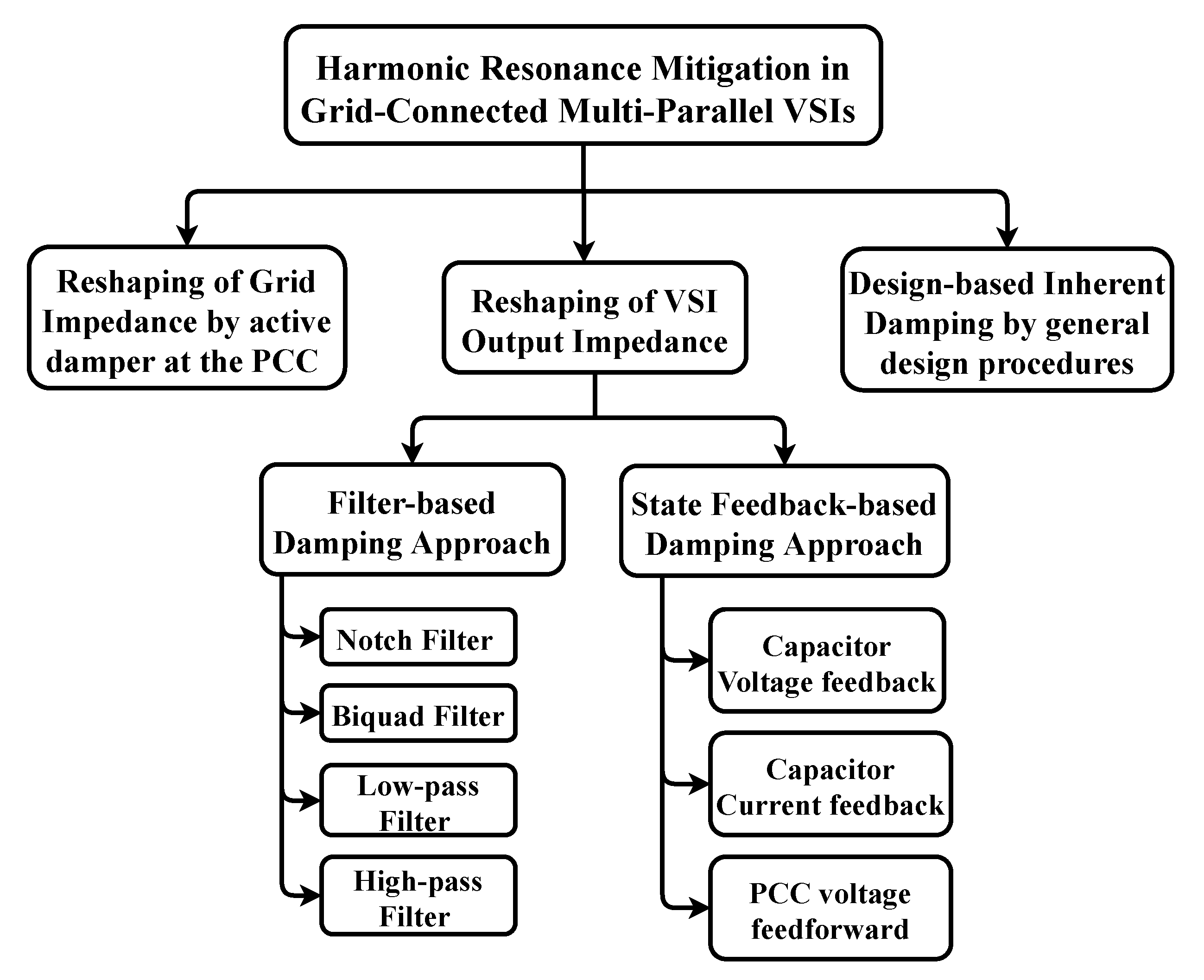
4. Suppression of Different Resonances in Multi–Parallel Grid–Connected Inverters

As discussed in the previous section, the resonances associated with the parallel VSIs are more challenging, as the VSI interacts externally with what can be considered as an active grid impedance formed by the differing dynamics of all of the other parallel inverters. As a result, the damping approaches used to attenuate the resonance of a single grid–connected VSI may no longer be applicable to the multi–parallel inverter case. This section reviews the approaches which have been developed to suppress the various resonances in the case of multi–paralleled grid–connected inverters.

Reshaping the inverter output impedance and reshaping the grid impedance are the two most common methods for reducing resonances. The addition of further control loops or compensation networks to the inverter’s control structure can be used to reshape its output impedance [59,60,61]. In a multi–parallel inverter system, the grid impedance that is seen by a particular VSI is the combination of the passive grid impedance and the impedances of the other parallel inverter [45]. The reshaping of the grid impedance can be adopted by adding additional hardware equipment to the PCC or introducing a virtual impedance in parallel with the grid impedance. Another approach to consider is the adoption of design rules to avoid the instability caused by the interaction between the inverters and the grid [62]. Figure 20 categorizes the various damping approaches that have been employed to mitigate the harmonic resonance in multi–parallel inverter system.

4.1. Reshaping of Inverter Output Impedance–Based Damping

The state–feedback–based approach and the filter-based technique are the two most commonly employed methods for altering the VSI output impedance. The state–feedback–based damping technique generally necessitates additional feedback signals with appropriate algorithms to imitate virtual impedances. On the other hand, the filter–based damping solution can typically be implemented without further measurements in the forward or feedback route of the current control loop.

4.1.1. State–Feedback–Based Damping Approach

The state–feedback–based damping technique typically depends on using one of the system state variables, such as capacitor voltage, capacitor current, or PCC feedforward voltage to mitigate the resonances in multiple grid–connected converter systems. For example, reference [38] proposes a combination of proportionate resonant (PR) control and full state feedback control of the capacitor voltage, the inverter-side current and the grid–side current. The proposed technique performed well when system characteristics such as the number of inverters and grid impedance changed. Full state feedback control necessitates the addition of extra internal feedback loops, which necessitates the installation of more sensors, raising the system cost. The control block diagram for the previously used example with the addition of various state–feedback–based damping methods is depicted in Figure 21.

Chen et al. in [63] proposed a virtual resistance in parallel with the filter capacitor. The value of the damping resistance is determined by the inverter–side inductor, the active damping coefficient of the LCL inherent resonance and the filter capacitor value. The virtual resistance–based method is able to suppress harmonic resonances in parallel inverter systems without deteriorating the filter dynamic in multiple frequency ranges, low and high frequency, unlike the physical damping resistance. In a further variation on the work in [63], the harmonic resonances in parallel inverter systems are dampened in [64] by using a virtual resistance in parallel with the filter capacitor. The filter capacitor voltage feedback is incorporated into the current control forward path in this investigation. The distinction between the two studies is the current controller, which is based on the PR current controller in the former and the deadbeat current controller in the later.

The impedance matching approach was adopted in [65] to conduct resonance suppression in the parallel inverter system. In this method, a virtual inductive–resistive impedance is created in parallel with the filter capacitor. Basically, the capacitor of the LCL filter introduces a harmonic resonance in specific frequency ranges due to the integration of the VSI-based LCL filter into the grid, which is primarily inductive. The harmonic resonance can be reduced by re-configuring the capacitive branch’s impedance to act like a resistance. This can be accomplished by adding a virtual inductive–resistive impedance to the filter capacitor in parallel. By locating the inductance and capacitive resonance frequency at the harmonic resonance frequency, a resistive equivalent impedance in the harmonic–frequency region can be achieved. However, the proposed strategy requires more sensors to measure both capacitor current and voltage in order to tune the feedback gains, although the estimation of the capacitor current based on the derivation of the filter capacitor voltage could simplify the system, necessitating the use of fewer sensors. Furthermore, unlike the prior approach, which puts a virtual resistance in the capacitive branch, this approach uses a virtual inductance to neutralize the capacitive branch’s effect. However, this approach does require some knowledge of the resonance frequency to tune the virtual inductance.

In [49], researchers described a graphical–based design approach for resonance mitigation in parallel inverter systems. The proposed technique takes into account the influence of control parameters such as controller gains and filter settings on the system stability. As a result, the variations in various parameters that could change at the same time and cause stability issues are considered. Based on the evaluation of the maximum real part of the system roots, which should be smaller than zero for stability, the boundary of the stability zone can be identified using an iterative technique. The active damping virtual resistance and current controller gain can be set using this stability region as a guide. Apart from its simplicity, the proposed technique is iterative and potentially time-consuming. Although the switching frequency, which is an important factor that influences the filter parameters, and the control bandwidth, were not taken into account, the method could be extended to accounts for these parameters.

The inverter output impedance was reconfigured in [66], also utilizing the virtual impedance method to reduce harmonic oscillation in the multi–parallel inverter system. To accomplish this, a PCC voltage feedforward path with a notch filter can create a virtual impedance in parallel with the inverter output impedance, which is low at the harmonic oscillation frequency, allowing the high–frequency harmonic current to flow into the parallel branch with lower impedance, effectively suppressing harmonic oscillations. Meanwhile, a notch filter in the grid–side inductor current feedback circuit introduces another virtual impedance in series with the inverter output impedance. At the fundamental frequency, this series impedance has a low value. Unlike the prior state feedback damping method, which relied on designing a suitable gain, this method relies on tuning a notch filter to achieve the damping. The proposed technique improves the stability of the parallel inverter system; nevertheless, using the notch filter in the control loop requires knowledge of the resonance frequency, which fluctuates depending on grid impedance, especially in weak grids.

Another technique for mitigation of harmonic resonances in multi–parallel grid–connected inverters was recently presented in [67,68]. The goal of this method is to cancel out the system’s entire parallel admittance by adding a virtual negative admittance to the target inverter. As a result, the total equivalent parallel admittance of the system is eliminated, and no harmonic resonances will exist. To accomplish this goal, a full PCC voltage feedforward technique is applied to only one of the parallel system’s inverters, rather than all of them. The proposed technique demonstrated a dependable performance despite grid impedance variations; however, its robustness is influenced by uncertainties or parameter modifications that may be added to the parallel inverter system. Due to these uncertainties and variances, the phase margin angle is reduced in contrast to the situation without the suggested PCC voltage feedforward, and the system’s suppression capability may be decreased.

The resonances in the parallel inverter system are dampened in [14] by using a predictive deadbeat control strategy. To reduce harmonic resonances, improved deadbeat control with a virtual harmonic resistance is used. The virtual resistance, which is calculated based on the desired damping ratio, is less sensitive to parameter changes and simulates the effect of passive damping via digital converter control. The established deadbeat control strategy has good steady-state and dynamic response properties, but being one of the predictive digital control approaches, an exact mathematical model is required. Furthermore, because the deadbeat current controller uses the inverter–side current as a control feedback, the grid side current’s power factor cannot be exactly controlled.

By flexibly engaging the active damping function, a bilevel framework with functional–rotation–based active dampers aiming to suppress harmonic resonances in a microgrid was suggested in [48]. In other words, the active damping strategy is implemented and distributed in some of the interface inverters rather than all of the parallel inverters, especially during microgrid reconfiguration. The proposed technique is bilevel rotation–based active damping, which means it has two levels: upper and lower control levels. The top control level is concerned with parallel inverter coordination and the selection of the appropriate inverter to implement and execute the active damping task in real–time. The lower control level is in charge of selecting the suitable value for the virtual damping resistor and detecting the resonance frequency of the paralleled inverters in order to properly perform active damping. Apart from the effectiveness of the proposed technique, the active damping approach should be created in a pre-selected inverter depending on the microgrid reconfiguration, where all the inverters in the microgrid can be coordinated. However, it may be difficult to implement in a larger distribution system. In addition, a communication port should be used to control the activation of the active damping in real–time in response to the microgrid reconfiguration, which adds expense in addition to the delay. As a result, the active damping approach is constrained by the communication delay time. As the communication delay time grows longer, the active damping technique may be unable to reduce resonance peaks.

Unlike the active damping options outlined previously, Yang [69] chose to suppress harmonic resonances in multi–parallel inverters through a passive approach. A suppression approach known as branch voltage and current double feedback was devised in this paper. Two passive resistors are used in this method, the first of which is coupled in series with the filter capacitor to improve high-frequency harmonic filtering capabilities. To strengthen the filter capacitor’s capacity to reduce low harmonics, the second damping resistor is connected in parallel with it. Apart from the proposed strategy’s good performance and the inverter’s control structure remaining unchanged, the proposed damping approach introduces continuous power losses that reduce the system’s overall efficiency.

4.1.2. Filter–Based Damping Approach

Several research papers have discussed the filter–based dampening approach. For instance, Tao et al. in [70] developed an active suppression strategy based on a digital notch filter which was designed and integrated into the capacitive current feedback active damping control to suppress the interactive resonance current in the multi–parallel inverter system. As the notch filter is designed to produce an anti–resonant peak opposite the interaction frequency, the instability can be reduced by fine–tuning the notch frequency. Meanwhile, the digital notch filter damping performance has no effect on the other frequency bands that are kept constant because the gain of the digital notch filter damping is zero throughout the other uninteresting frequency ranges. The notch filter’s fundamental flaw is its sensitivity to changes in filter resonance frequency, in addition to the significant negative phase shift that is generated at its characteristic frequency.

In [71], the resonant current is suppressed by using a biquad digital filter in the current control loop of the parallel inverters, as shown in Figure 22. The system’s stability is ensured by properly setting the biquad digital filter parameters, as unstable poles are concurrently pushed into the stable area. The system is cost-effective, since no new sensors are required, despite the increased number of biquad filter parameters that must be set.

The study in [72] proposes an active damping method based on a notch filter and a lag filter, based on industrial needs for the active damping design to suppress harmonic resonances in commercial inverters that are functioning in parallel. To begin, the main requirements of active damping are summarized as follows: the inverter’s execution time and changes in program code must be kept to a minimum, no additional sensors should be added, system robustness against grid impedance variations is a concern, the system bandwidth must be properly adjusted to ensure appropriate dynamics and the system must be able to operate in double-update mode (asymmetrical PWM). A notch filter was designed to boost the resilience against grid impedance fluctuations in order to meet these objectives. Furthermore, lag filter is employed to displace the phase angle at the resonance frequency; hence, the instability is mitigated and the system’s robustness is improved.

In [73], an enhanced notch filter is proposed to reshape the output impedance of the parallel inverters for resonance suppression while eliminating the substantial negative phase shift generated by the classic notch filter at its characteristic frequency. The notch filter modifies the current control loop in this work to raise the inverters’ output impedance by establishing a series virtual impedance with the inverter output impedance to attenuate the high-frequency oscillation. As a result of redesigning the inverter output impedance, the harmonic current injected into the grid by parallel inverters is kept stable.

The study in [74] created a damping approach based on the use of a low pass digital filter to add enough phase lag to stabilize the system when it comes to resonance damping in grid-connected inverters that work in parallel. To accomplish active damping, a Butterworth digital filter is applied to the current control loop. Despite the parallel inverter system’s excellent damping performance and established stability, a physical resistor should be added to improve the harmonic spectrum of the grid current as the system obtains additional damping, hence improving grid current power quality. On the other hand, the system’s efficiency could be compromised due to the additional losses.

The interactive resonant current among parallel inverters was reduced in [75] by cascading the traditional active damping loop with a proportional resonant controller, with phase compensation in each inverter. Although this damping method efficiently suppresses the circulating current, the PR controller seems to imply operation at a single resonant frequency, which requires some knowledge of the resonance frequency.

To ensure the stability of a multi–parallel inverter system that is connected to the grid, a high–pass filter was proposed in [76] to be implemented in a feedback current control loop, as depicted in Figure 23. As the grid impedance is not constant and must be computed in real–time, the proposed active damping approach graphically establishes the relative stability region before calculating the parameters of the high-pass filter and current controller, which may affect the system’s robustness.

The VSI’s control output admittance in [27] is broken down into a passive filter output admittance and an active admittance. The active admittance is influenced by the current controller and the time delay. For grid–side current feedback, the resonance frequency of the converter–side filter inductor and filter capacitor, the digital controller and PWM time delay constitute the stability region of the VSI. The resonance mitigation is performed by synthesizing damping controllers based on the discrete derivative controller to improve individual converters’ passivity. Instead of providing additional control loops, the damping controllers are embedded into the single–loop control structure, decreasing the number of sensors.

Model current predictive control (MCPC) and two-degree–of–freedom control were created in [77] to reduce resonances in multi–inverter parallel grid–connected inverters. As the MCPC’s value function comprises both the reference current of the control layer inner loop and the inverter output current, the present inner–loop PI current control layer and PWM module can be removed using this approach. The proposed method shows good suppression of various resonances. However, because this is a predictive control method, a precise mathematical model is required. In a similar vein, a resonance suppression method based on current model predictive control and two-degree–of–freedom control was developed in [78].

In [79], an improved predictive current controller is presented that achieves passive VSI output admittance over a high frequency range nearly up to the Nyquist frequency. The impact of the converter-side inductor value employed by the predictive controller on the VSI’s passive admittance range was investigated. For example, a larger inductor limits the passive range, but a smaller inductor, when compared to the real converter–side inductor, results in a wider passive admittance range, and hence superior damping capabilities. Meanwhile, as the inductor value decreases, the open–loop gain for current tracking decreases, increasing the steady-state inaccuracy. Second–order delayed feedback of the predictive controller output was designed to increase the passivity margin of the VSI output impedance and ensure a better phase margin over a wider frequency range. It has an effect on non-passive behavior near the fundamental frequency, but has no effect on phase at other frequencies. On the other hand, this damping approach is exclusively applied for the VSI with an inverter–side current controller, which is not widely employed due to inability to directly control the power factor on the grid side [80].

4.2. Resonance Damping Based on the Reshaping of Grid Impedance

In a multi–parallel inverter system, the grid impedance that is seen by a particular VSI is the combination of the passive grid impedance and the impedances of the other parallel inverter. Hence, the grid impedance is an active impedance instead of being passive. Therefore, the resonance in a multiparallel inverter system can be mitigated by reshaping the grid impedance rather than amending the output impedance of the parallel inverters. That is based on the practical assumption that the inverter control structure and parameters may be unknown, and the operator of the inverters–based plant cannot replace all the parallel inverters with new ones. To suppress the resonance problem, the grid impedance is modified by adding a device to the PCC or inserting a virtual impedance in parallel with the grid impedance.

In [45], an active damper based on a high bandwidth voltage source converter is used to suppress harmonic resonance in a multi–parallel inverter system. It is controlled to replicate a variable resistance at resonant frequencies caused by the grid’s interaction with the multi–paralleled inverter system. A resonance detecting system is used to create the variable resistance, which is based on the discrete Fourier transform (DFT) method. Although the resonance is effectively minimized by dynamically modifying the damper’s resonant frequency, the suggested damper resilience is heavily dependent on the precise resonant frequency identified in real–time, which is difficult to achieve. Furthermore, because this active damper is concerned with high-frequency resonances ranging from 800 Hz to 2 kHz, switching at a frequency greater than a conventional converter is needed to give the required control bandwidth for damping. It should also be noted that a higher voltage rating converter is required owing to its series ac L–filter, which has a bigger voltage drop than a standard shunt active power filter due to its higher frequency current flow, hence necessitating the need for a higher dc–link voltage.

The grid impedance is reshaped by a series LC–filtered active damper in [81] to reject grid disturbances and reduce harmonic resonances. The active damper was found to be effective at mitigating higher frequency resonances caused by interactions between several VSIs and the grid. In addition to the second–order resonant controller, a fourth–order resonant controller was used to reduce low-frequency harmonics. With strong damping performance at low rated voltage and faster switching operation, the suggested active damper in [81] outperformed its analog in [45]. As a series–connected extra capacitor was used to withstand most of the system voltage, the active damper can attenuate harmonic resonance with a lower voltage rating and a smaller filter, allowing for faster converter switching.

An active stabilizer based on an inductor filter-based rectifier that is linked at the PCC was used in [82] to reduce harmonic resonances in the multi–parallel inverters interfaced with the grid. Within the current controller bandwidth, the rectifier is regulated to imitate a resistive–inductive admittance. A substantial phase margin is obtained with this stabilizer, which improves the impedance stability of the multi–parallel inverter–grid system over a wide frequency range, ensuring overall system stability. It is worth noting that the proposed stabilizer’s shunt admittance is primarily determined by the inductor filter, which is chosen as a trade-off between current ripples and desired phase margin, resulting in an increase in the footprint of the passive element.

A global damper implemented at the PCC suppresses the harmonic resonance that occurs in grid–connected multi–parallel inverters in [83]. The damper is known as a thyristor switching RC (TSRC) damper because it is based on a passive RC circuit with a thyristor. The resistor’s primary role is to increase system damping by lowering harmonic resonance current, while the capacitor ensures that the damping resistor’s action is limited to the frequency of the resonance point.

In [84], both VSI and grid impedances are reshaped using a pure hardware approach. Local compensators are installed in series at the outputs of inverters, and common compensators are installed in series at the common outputs of multiple–paralleled inverters. The inverter output impedance is improved and harmonic currents are suppressed thanks to the local compensator. As for the grid impedance, the interactions between the multi–paralleled inverters always exist. Once the grid impedance reaches zero, the inverters are detached from one another. As the common compensator is employed, the equivalent grid impedance is canceled, and such interactions are removed. According to the findings, a common compensator could add virtual resistance into a multi–paralleled inverter system, causing a circulating current to circulate among the inverters. As a result, using a local compensator to reshape the inverter output impedance is preferred.

Reshaping the grid impedance can also be done by inserting a virtual impedance in parallel with the grid impedance. For example, the work in [85] used a band-pass filter to change the grid impedance by including a virtual admittance in parallel at the PCC. To avoid any negative impacts, this virtual admittance is substantial around the resonance frequency and significantly smaller at other frequencies. Despite the success of the proposed technique, the virtual admittance value is mostly determined by the grid impedance value, which varies unpredictably in real-time. As a result, because it is a parameter-sensitive procedure, the system’s robustness may be difficult to guarantee.

Although the general trend in the literature on this topic is to modify the inverter output impedance or the grid impedance, some researchers have also devised hybrid damping schemes that focus on both. The work in [86], for example, used a notch filter to reshape the inverter output impedance, and the grid impedance was molded by a centralized converter connected in parallel at the PCC. The active damper in the multi–parallel grid–connected inverters’ principal role is to produce a virtual impedance that is dynamically modified according to the resonance frequency. A second–order generalized-integrator frequency–locked–loop (SOGI–FLL) resonance detection approach is used to track the change in the system’s resonance frequency.

Despite the effectiveness of the previous damping strategy based on an active dampers, stabilisers, the cost of extra hardware, such as a converter and a passive element, has an impact on the overall cost of the damping system. It is also necessary to look at the likelihood of interactions between the active damper and the grid. Furthermore, because this approach is appropriate to a circumstance where the PCC of parallel inverters is common, such as a PV farm, it is not as applicable to a distribution grid where the parallel inverters are distributed.

4.3. Design-Based Inherent Damping

In a system with multiple inverters working in parallel, the suppression of resonance can be achieved by following a general design procedure for multi–parallel grid–connected inverter systems to avoid the instability. The damping approach in this scenario is known as design–based inherent damping. The work in [18] introduced output impedance constraints as a guide for the design of inverter controllers; hence, the harmonic interaction in a distorted grid is reduced. Moreover, the inherent damping in the parallel inverter system is provided in [62], where the control and circuit parameters are developed methodically. An extra LCL filter design requirement that considers both the lower and upper bounds of the combined resonant frequency range can be used to derive the inherent damping. Only if the grid impedance is inductive and resistive is this inherent damping strategy valid. On the other hand, if the grid impedance approaches capacitive impedance, as in the case of the dispersed capacitance of a very long transmission line, this approach is not applicable. Similarly, the research in [47] focused on the stability of grid-connected parallel inverters without the use of any additional dampening techniques. As the non–passive regions of the VSIs are different, it required the use of different LCL parameters, sampling frequencies and current control strategies of the inverters to obtain the inherent damping. As a result, these non–passive regions can cancel each other to ensure the overall stability of the power plant. The key drawback of this strategy is that all inverters have to be supplied from the same vendor or some sort of standard would have to be enforced, to guarantee the coordination between the inverters to gain the cancellation of the non-passive regions. Furthermore, all inverters must work together to maintain the passivity of the system.

In summary, a complete analysis of the different damping strategies used to minimize harmonic resonances in grid-connected parallel inverters is provided based on the above literature. The advantages and disadvantages of the various damping strategies are summarized in

Table 2. Comparison of different damping approaches.

Damping Strategy	Concept	Approach	Pros	Cons
Reshaping the inverter output impedance	State variable feedback–based damping (Virtual impedance–based damping) [49,63,64,65,66,67,68]	Full PCC voltage feedforward. Capacitor voltage feedback. Capacitor current feedback.	Simple implementation. Perfect damping performance. No additional losses. Ensuring the stability of the current control loop. Improving the VSI–grid system interaction stability.	Requires additional sensors. Sensitive to control delay and is restricted by control bandwidth. Influences the tracking accuracy of the inverter output power. Poor adaptability to the grid impedance variation. Some knowledge of the resonance frequency is required.
	Filter–based damping [70,71,72,74,75]	Notch filter. Biquad filter. Low pass filter. PR controller with phase compensation.	No additional sensors or passive elements. Strong and effective suppression performance against the resonance peak. Independent of grid impedance variation. High frequency noises are attenuated.	Robustness can be challenged by the variation of filter resonance frequency. Significant negative phase shift is generated at filter characteristic frequency. Some filters has increased number of parameters that complicate the design procedures.
Reshaping the grid impedance	Active damper [45,81,82,83,84]	Adding an additional converter at the PCC	Low power rating. Preferred strategy if the control structure and parameters are unknown.	Increased cost of the overall system. It relies on real–time detection of resonance frequency. High switching frequency is needed. Interaction between the active damper and the grid is a concern. Appropriate only where the PCC of the parallel inverters is determined.
Inherent damping–based system [47,62]	General design procedure for multi–parallel inverter systems	Developing the control and filter parameters methodically	Cost–effective. Simple approach.	Valid only for a resistive–inductive grid impedance

. Reshaping the grid impedance appears to be more feasible in terms of, for example, a PV farm that has already been installed and a PCC that has been determined; however, the expense of this solution has to be investigated further. When regarded as a preventive intervention during the design and implementation phase, however, reshaping the inverter output impedance is a more cost–effective choice. Furthermore, because parallel inverters are widely spread, it is more ideal for use in distribution networks where the PCC is unknown.

5. Conclusions

This paper provides a complete review of the analysis and mitigation approaches for various types of resonances in the multi–parallel grid–connected VSI. The concepts underlying the interactions in a multi–parallel inverter grid system have been described and illustrated with an example. The state–of–the–art damping approaches for the resonances resulting from the interactions have been comprehensively described; the advantages and disadvantages of all damping techniques have been summarized. By way of conclusion, impedance interactions in a grid with multiple parallel–connected inverters are certainly an issue of concern which could potentially lead to grid instability or at the very least a deterioration in power quality. On the positive side, a wide range of solutions have been devised to mitigate the issues, and most of these solutions have been shown to be effective at least under somewhat idealized laboratory conditions. However, the comparative effectiveness of the various solutions under the wide diversity of conditions and situations which are likely to be encountered in the real world is uncertain and certainly merits further study. The impact of power electronics trends, such as the use of wide bandgap semicondcutors and the use of new converter topologies, is also an area for future research. From a practical perspective, standards and associated test procedures for screening for interactions may need further development or updating in order to ensure that appropriate mitigation techniques are implemented in grid–connected inverters.

References

1. Cook, J.; Oreskes, N.; Doran, P.T.; Anderegg, W.R.; Verheggen, B.; Maibach, E.W.; Carlton, J.S.; Lewandowsky, S.; Skuce, A.G.; Green, S.A.; et al. Consensus on consensus: A synthesis of consensus estimates on human-caused global warming. Environ. Res. Lett. 2016, 11, 048002. [Google Scholar] [CrossRef]
2. United Nations Treaty Collection. Chapter XXBII. In 7.d Paris Agreement; United Nations Treaty Collection: New York, NY, USA, 2015; p. 12. [Google Scholar]
3. Murdock, H.E.; Gibb, D.; Andre, T.; Sawin, J.L.; Brown, A.; Ranalder, L.; Collier, U.; Dent, C.; Epp, B.; Hareesh Kumar, C.; et al. Renewables 2021—Global Status Report. 2021. Available online: https://www.ren21.net/wp-content/uploads/2019/05/GSR2021_Full_Report.pdf (accessed on 22 July 2022).
4. Blaabjerg, F.; Yang, Y.; Ma, K.; Wang, X. Power electronics-the key technology for renewable energy system integration. In Proceedings of the 2015 International Conference on Renewable Energy Research and Applications (ICRERA), Palermo, Italy, 22–25 November 2015; pp. 1618–1626. [Google Scholar]
5. Agorreta, J.L.; Borrega, M.; López, J.; Marroyo, L. Modeling and control of N-paralleled grid-connected inverters with LCL filter coupled due to grid impedance in PV plants. IEEE Trans. Power Electron. 2010, 26, 770–785. [Google Scholar] [CrossRef]
6. Enslin, J.H.; Heskes, P.J. Harmonic interaction between a large number of distributed power inverters and the distribution network. IEEE Trans. Power Electron. 2004, 19, 1586–1593. [Google Scholar] [CrossRef]
7. Li, C. Unstable operation of photovoltaic inverter from field experiences. IEEE Trans. Power Deliv. 2017, 33, 1013–1015. [Google Scholar] [CrossRef]
8. Liu, Q.; Liu, F.; Zou, R.; Li, Y. Harmonic Resonance Characteristic of Large-scale PV Plant: Modelling, Analysis and Engineering Case. IEEE Trans. Power Deliv. 2022, 37, 2359–2368. [Google Scholar] [CrossRef]
9. Gomes, C.C.; Cupertino, A.F.; Pereira, H.A. Damping techniques for grid-connected voltage source converters based on LCL filter: An overview. Renew. Sustain. Energy Rev. 2018, 81, 116–135. [Google Scholar] [CrossRef]
10. Wu, W.; Liu, Y.; He, Y.; Chung, H.S.H.; Liserre, M.; Blaabjerg, F. Damping methods for resonances caused by LCL-filter-based current-controlled grid-tied power inverters: An overview. IEEE Trans. Ind. Electron. 2017, 64, 7402–7413. [Google Scholar] [CrossRef] [Green Version]
11. Beres, R.N.; Wang, X.; Liserre, M.; Blaabjerg, F.; Bak, C.L. A review of passive power filters for three-phase grid-connected voltage-source converters. IEEE J. Emerg. Sel. Top. Power Electron. 2015, 4, 54–69. [Google Scholar] [CrossRef] [Green Version]
12. Zhang, C.; Dragicevic, T.; Vasquez, J.C.; Guerrero, J.M. Resonance damping techniques for grid-connected voltage source converters with LCL filters—A review. In Proceedings of the 2014 IEEE International Energy Conference (ENERGYCON), Dubrovnik, Croatia, 13–16 May 2014; pp. 169–176. [Google Scholar]
13. Han, Y.; Yang, M.; Li, H.; Yang, P.; Xu, L.; Coelho, E.A.A.; Guerrero, J.M. Modeling and stability analysis of LCL-type grid-connected inverters: A comprehensive overview. IEEE Access 2019, 7, 114975–115001. [Google Scholar] [CrossRef]
14. He, J.; Li, Y.W.; Bosnjak, D.; Harris, B. Investigation and active damping of multiple resonances in a parallel-inverter-based microgrid. IEEE Trans. Power Electron. 2012, 28, 234–246. [Google Scholar] [CrossRef]
15. Sun, J. Small-signal methods for AC distributed power systems—A review. IEEE Trans. Power Electron. 2009, 24, 2545–2554. [Google Scholar]
16. Wang, Y.; Wang, X.; Chen, Z.; Blaabjerg, F. Small-signal stability analysis of inverter-fed power systems using component connection method. IEEE Trans. Smart Grid 2017, 9, 5301–5310. [Google Scholar] [CrossRef] [Green Version]
17. Amin, M.; Molinas, M. Small-signal stability assessment of power electronics based power systems: A discussion of impedance-and eigenvalue-based methods. IEEE Trans. Ind. Appl. 2017, 53, 5014–5030. [Google Scholar] [CrossRef]
18. Wang, F.; Duarte, J.L.; Hendrix, M.A.; Ribeiro, P.F. Modeling and analysis of grid harmonic distortion impact of aggregated DG inverters. IEEE Trans. Power Electron. 2010, 26, 786–797. [Google Scholar] [CrossRef]
19. He, Y.; Wang, X.; Pan, D.; Ruan, X.; Su, G. An Ignored Culprit of Harmonic Oscillation in LCL-Type Grid-Connected Inverter: Resonant Pole Cancelation. IEEE Trans. Power Electron. 2021, 36, 14282–14294. [Google Scholar] [CrossRef]
20. Chen, H.c.; Cheng, P.t.; Wang, X.; Blaabjerg, F. A passivity-based stability analysis of the active damping technique in the offshore wind farm applications. IEEE Trans. Ind. Appl. 2018, 54, 5074–5082. [Google Scholar] [CrossRef] [Green Version]
21. Sun, J. Impedance-based stability criterion for grid-connected inverters. IEEE Trans. Power Electron. 2011, 26, 3075–3078. [Google Scholar] [CrossRef]
22. Ali, R.; O’Donnell, T. Parameters Influencing Harmonic Stability for Single-phase Inverter in the Low Voltage Distribution Network. In Proceedings of the 2021 IEEE PES Innovative Smart Grid Technologies Europe (ISGT Europe), Espoo, Finland, 18–21 October 2021; pp. 1–5. [Google Scholar]
23. Yu, Y.; Li, H.; Li, Z.; Zhao, Z. Modeling and analysis of resonance in LCL-type grid-connected inverters under different control schemes. Energies 2017, 10, 104. [Google Scholar] [CrossRef] [Green Version]
24. Sowa, I.; Domínguez-García, J.L.; Gomis-Bellmunt, O. Impedance-based analysis of harmonic resonances in HVDC connected offshore wind power plants. Electr. Power Syst. Res. 2019, 166, 61–72. [Google Scholar] [CrossRef]
25. Jia, L.; Ruan, X.; Zhao, W.; Lin, Z.; Wang, X. An adaptive active damper for improving the stability of grid-connected inverters under weak grid. IEEE Trans. Power Electron. 2018, 33, 9561–9574. [Google Scholar] [CrossRef]
26. Harnefors, L.; Bongiorno, M.; Lundberg, S. Input-admittance calculation and shaping for controlled voltage-source converters. IEEE Trans. Ind. Electron. 2007, 54, 3323–3334. [Google Scholar] [CrossRef]
27. Wang, X.; Blaabjerg, F.; Loh, P.C. Passivity-based stability analysis and damping injection for multi–paralleled VSCs with LCL filters. IEEE Trans. Power Electron. 2017, 32, 8922–8935. [Google Scholar] [CrossRef] [Green Version]
28. Hans, F.; Schumacher, W.; Chou, S.F.; Wang, X. Passivation of current-controlled grid-connected VSCs using passivity indices. IEEE Trans. Ind. Electron. 2018, 66, 8971–8980. [Google Scholar] [CrossRef]
29. Harnefors, L.; Wang, X.; Yepes, A.G.; Blaabjerg, F. Passivity-based stability assessment of grid-connected VSCs—An overview. IEEE J. Emerg. Sel. Top. Power Electron. 2015, 4, 116–125. [Google Scholar] [CrossRef] [Green Version]
30. Han, Y.; Yang, M.; Yang, P.; Xu, L.; Blaabjerg, F. Passivity-based stability analysis of parallel single-phase inverters with hybrid reference frame control considering PLL effect. Int. J. Electr. Power Energy Syst. 2022, 135, 107473. [Google Scholar] [CrossRef]
31. Ma, J.; Wang, X.; Blaabjerg, F.; Song, W.; Wang, S.; Liu, T. Multisampling method for single-phase grid-connected cascaded H-bridge inverters. IEEE Trans. Ind. Electron. 2019, 67, 8322–8334. [Google Scholar] [CrossRef]
32. Zhang, X.; Chen, P.; Yu, C.; Li, F.; Do, H.T.; Cao, R. Study of a current control strategy based on multisampling for high-power grid-connected inverters with an LCL filter. IEEE Trans. Power Electron. 2016, 32, 5023–5034. [Google Scholar] [CrossRef]
33. Roy, T.K.; Mahmud, M.A.; Islam, S.; Oo, A.M. Power quality improvements in single-phase grid-connected photovoltaic systems using a nonlinear adaptive controller. In Proceedings of the 2018 Australasian Universities Power Engineering Conference (AUPEC), Auckland, New Zealand, 27–30 November 2018; pp. 1–6. [Google Scholar]
34. Gui, Y.; Wang, X.; Wu, H.; Blaabjerg, F. Voltage-modulated direct power control for a weak grid-connected voltage source inverters. IEEE Trans. Power Electron. 2019, 34, 11383–11395. [Google Scholar] [CrossRef] [Green Version]
35. Sun, J.; Wang, G.; Du, X.; Wang, H. A theory for harmonics created by resonance in converter-grid systems. IEEE Trans. Power Electron. 2018, 34, 3025–3029. [Google Scholar] [CrossRef]
36. Lu, M.; Wang, X.; Blaabjerg, F.; Loh, P.C. An analysis method for harmonic resonance and stability of multi-paralleled LCL-filtered inverters. In Proceedings of the 2015 IEEE 6th International Symposium on Power Electronics for Distributed Generation Systems (PEDG), Aachen, Germany, 22–25 June 2015; pp. 1–6. [Google Scholar]
37. Lu, M.; Wang, X.; Loh, P.C.; Blaabjerg, F. Resonance interaction of multiparallel grid-connected inverters with LCL filter. IEEE Trans. Power Electron. 2016, 32, 894–899. [Google Scholar] [CrossRef]
38. Tan, S.; Yang, G.; Geng, H.; Ma, S.; Wu, W. A resonance suppression method for a multiple grid-connected-converter system with LCL filter. In Proceedings of the 2014 International Power Electronics and Application Conference and Exposition, Shanghai, China, 5–8 November 2014; pp. 1104–1109. [Google Scholar]
39. Ciobotaru, M.; Teodorescu, R.; Blaabjerg, F. A new single-phase PLL structure based on second order generalized integrator. In Proceedings of the 2006 37th IEEE Power Electronics Specialists Conference, Jeju, Korea, 18–22 June 2006; pp. 1–6. [Google Scholar]
40. Yang, Z.; Shah, C.; Chen, T.; Yu, L.; Joebges, P.; De Doncker, R.W. Stability investigation of three-phase grid-tied pv inverter systems using impedance models. IEEE J. Emerg. Sel. Top. Power Electron. 2022, 10, 2672–2684. [Google Scholar] [CrossRef]
41. Teodorescu, R.; Blaabjerg, F.; Liserre, M.; Loh, P.C. Proportional-resonant controllers and filters for grid-connected voltage-source converters. IEE Proc.-Electr. Power Appl. 2006, 153, 750–762. [Google Scholar] [CrossRef] [Green Version]
42. Zhou, S.; Zou, X.; Zhu, D.; Tong, L.; Zhao, Y.; Kang, Y.; Yuan, X. An improved design of current controller for LCL-type grid-connected converter to reduce negative effect of PLL in weak grid. IEEE J. Emerg. Sel. Top. Power Electron. 2017, 6, 648–663. [Google Scholar] [CrossRef]
43. Khajeh, K.G.; Solatialkaran, D.; Zare, F.; Mithulananthan, N. Harmonic analysis of multi-parallel grid-connected inverters in distribution networks: Emission and immunity issues in the frequency range of 0–150 kHz. IEEE Access 2020, 8, 56379–56402. [Google Scholar] [CrossRef]
44. Barsali, S. Benchmark Systems for Network Integration of Renewable and Distributed Energy Resources; International Council on Large Electric Systems: Paris, France, 2014. [Google Scholar]
45. Wang, X.; Blaabjerg, F.; Liserre, M.; Chen, Z.; He, J.; Li, Y. An active damper for stabilizing power-electronics-based AC systems. IEEE Trans. Power Electron. 2013, 29, 3318–3329. [Google Scholar] [CrossRef]
46. Qian, Q.; Xie, S.; Huang, L.; Xu, J.; Zhang, Z.; Zhang, B. Harmonic suppression and stability enhancement for parallel multiple grid-connected inverters based on passive inverter output impedance. IEEE Trans. Ind. Electron. 2017, 64, 7587–7598. [Google Scholar] [CrossRef]
47. Bai, H.; Wang, X.; Blaabjerg, F. Passivity enhancement in renewable energy source based power plant with paralleled grid-connected VSIs. IEEE Trans. Ind. Appl. 2017, 53, 3793–3802. [Google Scholar] [CrossRef]
48. Guo, Y.; Lu, X.; Chen, L.; Zheng, T.; Wang, J.; Mei, S. Functional-rotation-based active dampers in AC microgrids with multiple parallel interface inverters. IEEE Trans. Ind. Appl. 2018, 54, 5206–5215. [Google Scholar] [CrossRef]
49. Guo, Y.; Chen, L.; Lu, X.; Wang, J.; Zheng, T.; Mei, S. Region Based Stability Analysis of Active Dampers in AC Microgrids with Multiple Parallel Interface Inverters. In Proceedings of the 2019 IEEE Applied Power Electronics Conference and Exposition (APEC), Anaheim, CA, USA, 17–21 March 2019; pp. 1098–1101. [Google Scholar]
50. Yamashita, K.; Villanueva, S.M.; Cutsem, T.V.; Martins, J.C.; Song, Z.; Zhu, L.; Renner, H.; Aristidou, P.; Green, I.; Lammert, G.; et al. Modelling of Inverter-Based Generation for Power System Dynamic Studies; CIGRE: Paris, France, 2018. [Google Scholar]
51. Qiu, Q.; Huang, Y.; Ma, R.; Kurths, J.; Zhan, M. Black-Box Impedance Prediction of Grid-Tied VSCs Under Variable Operating Conditions. IEEE Access 2021, 10, 1289–1304. [Google Scholar] [CrossRef]
52. Cifuentes, N.; Sun, M.; Gupta, R.; Pal, B.C. Black-Box Impedance-Based Stability Assessment of Dynamic Interactions Between Converters and Grid. IEEE Trans. Power Syst. 2021, 37, 2976–2987. [Google Scholar] [CrossRef]
53. De Meerendre, M.K.; Prieto-Araujo, E.; Ahmed, K.H.; Gomis-Bellmunt, O.; Xu, L.; Egea-Àlvarez, A. Review of local network impedance estimation techniques. IEEE Access 2020, 8, 213647–213661. [Google Scholar] [CrossRef]
54. Ahmed, S.; Shen, Z.; Mattavelli, P.; Boroyevich, D.; Karimi, K.J. Small-signal model of voltage source inverter (VSI) and voltage source converter (VSC) considering the deadtime effect and space vector modulation types. IEEE Trans. Power Electron. 2016, 32, 4145–4156. [Google Scholar] [CrossRef]
55. Shi, H.; Zhuo, F.; Zhang, D.; Geng, Z.; Wang, F. Modeling, analysis, and measurement of impedance for three-phase AC distributed power system. In Proceedings of the 2014 IEEE Energy Conversion Congress and Exposition (ECCE), Pittsburgh, PA, USA, 14–18 September 2014; pp. 4635–4639. [Google Scholar]
56. Capponi, L.; Fernández, I.; Roggo, D.; Arrinda, A.; Angulo, I.; De La Vega, D. Comparison of measurement methods of grid impedance for narrow band-PLC up to 500 kHz. In Proceedings of the 2018 IEEE 9th International Workshop on Applied Measurements for Power Systems (AMPS), Bologna, Italy, 26–28 September 2018; pp. 1–6. [Google Scholar]
57. Rhode, J.P.; Kelley, A.W.; Baran, M.E. Complete characterization of utilization-voltage power system impedance using wideband measurement. IEEE Trans. Ind. Appl. 1997, 33, 1472–1479. [Google Scholar] [CrossRef]
58. Shah, S.; Koralewicz, P.; Gevorgian, V.; Liu, H.; Fu, J. Impedance methods for analyzing stability impacts of inverter-based resources: Stability analysis tools for modern power systems. IEEE Electrif. Mag. 2021, 9, 53–65. [Google Scholar] [CrossRef]
59. Xueguang, Z.; Li, W.; Xiao, Y.; Wang, G.; Xu, D. Analysis and suppression of circulating current caused by carrier phase difference in parallel voltage source inverters with SVPWM. IEEE Trans. Power Electron. 2018, 33, 11007–11020. [Google Scholar] [CrossRef]
60. Yang, D.; Ruan, X.; Wu, H. Impedance shaping of the grid-connected inverter with LCL filter to improve its adaptability to the weak grid condition. IEEE Trans. Power Electron. 2014, 29, 5795–5805. [Google Scholar] [CrossRef]
61. Chen, X.; Zhang, Y.; Wang, S.; Chen, J.; Gong, C. Impedance-phased dynamic control method for grid-connected inverters in a weak grid. IEEE Trans. Power Electron. 2016, 32, 274–283. [Google Scholar] [CrossRef]
62. Chen, T.; Lee, C.K.; Hui, S.R. A general design procedure for multi-parallel modular grid-tied inverters system to prevent common and interactive instability. IEEE Trans. Power Electron. 2019, 34, 6025–6030. [Google Scholar] [CrossRef]
63. Chen, Z.; Chen, Y.; Guerrero, J.M.; Kuang, H.; Huang, Y.; Zhou, L.; Luo, A. Generalized coupling resonance modeling, analysis, and active damping of multi-parallel inverters in microgrid operating in grid-connected mode. J. Mod. Power Syst. Clean Energy 2016, 4, 63–75. [Google Scholar] [CrossRef] [Green Version]
64. Chen, Z.; Luo, A.; Chen, Y.; Li, M. Resonance features of multi-paralleled grid-connected inverters and its damping method. In Proceedings of the 2014 International Power Electronics and Application Conference and Exposition, Shanghai, China, 5–8 November 2014; pp. 120–125. [Google Scholar]
65. Tan, S.; Geng, H.; Yang, G. Impedance matching based control for the resonance damping of microgrids with multiple grid connected converters. J. Power Electron. 2016, 16, 2338–2349. [Google Scholar] [CrossRef] [Green Version]
66. Yang, L.; Chen, Y.; Wang, H.; Luo, A.; Huai, K. Oscillation suppression method by two notch filters for parallel inverters under weak grid conditions. Energies 2018, 11, 3441. [Google Scholar] [CrossRef] [Green Version]
67. Gharanikhajeh, K.; Solatialkaran, D.; Zare, F.; Faradjizadeh, F.; Yaghoobi, J.; Nadarajah, M. A Harmonic Mitigation Technique for Multi-Parallel Grid-Connected Inverters in Distribution Networks. IEEE Trans. Power Deliv. 2022, 37, 2843–2856. [Google Scholar]
68. Khajeh, K.G.; Farajizadeh, F.; Solatialkaran, D.; Zare, F.; Yaghoobi, J.; Nadarajah, M. A Full-Feedforward Technique to Mitigate the Grid Distortion Effect on Parallel Grid-Tied Inverters. IEEE Trans. Power Electron. 2022, 37, 8404–8419. [Google Scholar] [CrossRef]
69. Yang, Q.X.; Li, K.; Zhao, C.M.; Wang, H. The resonance suppression for parallel photovoltaic grid-connected inverters in weak grid. Int. J. Autom. Comput. 2018, 15, 716–727. [Google Scholar] [CrossRef]
70. Tao, H.; Zhou, Y.; Zhang, G.; Zheng, Z. Parallel Resonance Mechanism Analysis and Suppression of Inductance-Capacitance-Inductance Grid-Connected Inverters. Energies 2019, 12, 1656. [Google Scholar] [CrossRef] [Green Version]
71. Lu, X.; Sun, K.; Huang, L.; Liserre, M.; Blaabjerg, F. An active damping method based on biquad digital filter for parallel grid-interfacing inverters with LCL filters. In Proceedings of the 2014 IEEE Applied Power Electronics Conference and Exposition—APEC 2014, Fort Worth, TX, USA, 16–20 March 2014; pp. 392–397. [Google Scholar]
72. Pena-Alzola, R.; Roldán-Pérez, J.; Bueno, E.; Huerta, F.; Campos-Gaona, D.; Liserre, M.; Burt, G. Robust active damping in LCL-filter-based medium-voltage parallel grid inverters for wind turbines. IEEE Trans. Power Electron. 2018, 33, 10846–10857. [Google Scholar] [CrossRef] [Green Version]
73. Yang, L.; Chen, Y.; Luo, A.; Huai, K. Stability enhancement for parallel grid-connected inverters by improved notch filter. IEEE Access 2019, 7, 65667–65678. [Google Scholar] [CrossRef]
74. Samanes, J.; Gubía, E. Sensorless active damping strategy for parallel interleaved voltage source power converters with LCL filter. In Proceedings of the 2017 IEEE Applied Power Electronics Conference and Exposition (APEC), Tampa, FL, USA, 26–30 March 2017; pp. 3632–3639. [Google Scholar]
75. Qian, Q.; Zhang, B.; Ni, Z.; Xie, S.; Xu, J.; Xu, K. Circulating resonant current suppression for current-controlled inverters based on output impedance shaping. In Proceedings of the 2017 IEEE Energy Conversion Congress and Exposition (ECCE), Cincinnati, OH, USA, 1–5 October 2017; pp. 4794–4798. [Google Scholar]
76. Liang, J.; Jiang, J.; Ojo, O.; Haruna, J. Damping for Multi-Paralleled Grid Tied Inverters with LCL Filters. In Proceedings of the 2018 IEEE Energy Conversion Congress and Exposition (ECCE), Portland, OR, USA, 23–27 September 2018; pp. 5879–5886. [Google Scholar]
77. Zheng, F.; Lin, X.; Zhang, Y.; Deng, C. Design of a novel hybrid control strategy for multi-inverter parallel system for resonance suppression. Energy Sci. Eng. 2020, 8, 2878–2893. [Google Scholar] [CrossRef]
78. Li, D.; Chen, M.; Yang, W.; Lin, X. A Novel Hybrid Control Algorithm for Suppressing the Resonance of Multiple Inverters in Parallel. In Proceedings of the 2020 IEEE/IAS Industrial and Commercial Power System Asia (I& CPS Asia), Weihai, China, 13–16 July 2020; pp. 1186–1191. [Google Scholar]
79. Awal, M.; Yu, W.; Husain, I. Passivity-based predictive-resonant current control for resonance damping in LCL-equipped VSCs. IEEE Trans. Ind. Appl. 2019, 56, 1702–1713. [Google Scholar] [CrossRef]
80. Zhou, X.; Lu, S. A novel inverter-side current control method of LCL-filtered inverters based on high-pass-filtered capacitor voltage feedforward. IEEE Access 2020, 8, 16528–16538. [Google Scholar] [CrossRef]
81. Wang, X.; Pang, Y.; Loh, P.C.; Blaabjerg, F. A series-LC-filtered active damper with grid disturbance rejection for AC power-electronics-based power systems. IEEE Trans. Power Electron. 2014, 30, 4037–4041. [Google Scholar] [CrossRef] [Green Version]
82. Zheng, C.; Zhou, L.; Xie, B.; Zhang, Q.; Li, H. A stabilizer for suppressing harmonic resonance in multi-parallel inverter system. In Proceedings of the 2017 IEEE Transportation Electrification Conference and Expo, Asia-Pacific (ITEC Asia-Pacific), Harbin, China, 7–10 August 2017; pp. 1–6. [Google Scholar]
83. Wan, Q.; Zhang, H. Research on resonance mechanism and suppression technology of photovoltaic cluster inverter. Energies 2018, 11, 938. [Google Scholar] [CrossRef] [Green Version]
84. Peng, Y.; He, Y.; Hang, L. Active Compensator for Multi-Paralleled Grid-Tied Inverters under variable Grid Conditions. In Proceedings of the 2019 IEEE Energy Conversion Congress and Exposition (ECCE), Baltimore, MD, USA, 29 September–3 October 2019; pp. 2629–2636. [Google Scholar]
85. Sun, J.j.; Hu, W.; Zhou, H.; Jiang, Y.M.; Zha, X.M. A resonant characteristics analysis and suppression strategy for multiple parallel grid-connected inverters with LCL filter. J. Power Electron. 2016, 16, 1483–1493. [Google Scholar] [CrossRef] [Green Version]
86. Yuan, C.; Shi, D.; Hu, Q.; Liao, Y.; Yu, J.; Zhou, P. Active Damping Resonance Suppression and Optimization of Photovoltaic Cluster Grid Connected System. J. Electr. Eng. Technol. 2021, 16, 2509–2521. [Google Scholar] [CrossRef]
Figure 1. Admittance model of grid–connected VSI.
Energies 15 05438 g001
Figure 2. Equivalent admittance model of grid–connected multi–parallel inverters.
Energies 15 05438 g002
Figure 3. Equivalent admittance model for the contribution made by the inverter from its own current source.
Energies 15 05438 g003
Figure 4. Admittance model for contributions from all of the other parallel connected inverters.
Energies 15 05438 g004
Figure 5. Equivalent admittance model for the impact of the utility grid voltage on the injected current.
Energies 15 05438 g005
Figure 6. Configuration of multi–paralleled LCL grid–connected inverters system.
Energies 15 05438 g006
Figure 7. System diagram of the detailed description of the single inverter system.
Energies 15 05438 g007
Figure 8. Control block diagram of grid current control for LCL grid–connected VSI.
Energies 15 05438 g008
Figure 9. Stable (a,c,e) and unstable (b,d,f) cases of a single inverter connected to the grid. (a,b) Bode plot of Y o and Y g . (c,d) Simulation results of the grid current waveforms. (e,f) Harmonic spectrum of grid current.
Energies 15 05438 g009
Figure 10. Main current resonance of the inverter itself in a multi–parallel inverter system.
Energies 15 05438 g010
Figure 11. Frequency response of the interactive current resonance among the VSIs.
Energies 15 05438 g011
Figure 12. Grid voltage current resonance between the parallel VSIs and the utility grid.
Energies 15 05438 g012
Figure 13. Bode plot of admittances of two identical parallel VSIs connected to the grid.
Energies 15 05438 g013
Figure 14. Simulation results of two identical parallel VSIs connected to the grid. (a) Grid current waveform. (b) Harmonic spectrum of grid current.
Energies 15 05438 g014
Figure 15. Bode plot of admittances of four identical parallel VSIs connected to the grid.
Energies 15 05438 g015
Figure 16. Simulation results of four identical parallel VSIs connected to the grid. (a) Grid current waveform. (b) Harmonic spectrum of grid current.
Energies 15 05438 g016
Figure 17. Bode plot of admittances of three different parallel VSIs connected to the grid.
Energies 15 05438 g017
Figure 18. Equivalent impedance model of four identical inverters with the impact of the additional impedances between the connection points.
Energies 15 05438 g018
Figure 19. Bode plot of output admittance of inverter 1 and the admittance of the equivalent grid with the additional impedances between the connection points.
Energies 15 05438 g019
Figure 20. Different damping approaches for harmonic resonance mitigation in a multi–parallel inverter system.
Energies 15 05438 g020
Figure 21. Control block diagram of different state–feedback–based damping methods.
Energies 15 05438 g021
Figure 22. Control block diagram of the biquad filter–based damping.
Energies 15 05438 g022
Figure 23. Control block diagram of high pass filter–based damping.
Energies 15 05438 g023