Robust Controller Considering Road Disturbances for a Vehicular Flywheel Battery System

Abstract

At present, the stability study of the flywheel battery system under the influence of road conditions is only limited to the analysis of dynamic characteristics but also lacks effective controller considering road disturbances. In order to solve this defect and further improve the robust performance of vehicular flywheel battery systems under road disturbances, a robust controller considering interference of road surface roughness is proposed. Firstly, on the basis of a brief introduction to flywheel battery system structure, the influence degree of the flywheel by road condition is compared to find the key areas most affected by road disturbance factors. Then the nonlinear dynamic model of the axial suspension system is constructed, and the actual road surface roughness is regarded as the unmodeled dynamics of the external disturbance emphatically. Following, the established unknown system dynamics is approximated by radial basis function (RBF) neural network based on the minimum parameter learning method, the control input is generated by sliding-mode control law, and the weight adjustment of neural network is replaced by the designed adaptive law of parameter estimation. The effects of different levels of road surface roughness on the system are simulated, and the robustness of the proposed controller is verified based on the Lyapunov method. Finally, the experimental platform to simulate road disturbances is designed ingeniously. Experimental results show that the proposed controller can make the flywheel battery system have good robustness under different road conditions.

1. Introduction

A vehicular battery system is a power battery with great development potential in the field of new energy vehicles [1,2]. As the key link of the flywheel battery system, the stability control performance of the magnetic suspension support-flywheel rotor system directly affects the operation quality of the whole flywheel battery system under external disturbances [3,4]. The disturbance source mainly comes from two aspects: on the one hand, it comes from the influence of the vehicle’s own driving conditions (starting, braking, acceleration, deceleration, uphill, turning, etc.) on the stability of the flywheel, which can be regarded as instantaneous disturbance; on the other hand, it comes from the road conditions of vehicles (different road levels) on the stability of flywheel, which can be regarded as the continuous disturbance. However, for the vehicle-mounted flywheel battery system, the disturbance from the road surface is continuous and inevitable because the vehicle runs on different road surface levels. Therefore, compared with the stability that can be restored to the original state by instantaneous disturbance, for the vehicle-mounted flywheel battery system, the robustness (the ability to maintain its original state under continuous perturbation) is a more critical factor.

At present, the influence of road conditions on the stability of the flywheel battery system has been studied. In [5], the impact of harmonic road disturbances on active magnetic bearing supported flywheel energy storage system in electric vehicles is analyzed. In [6], the influence of the magnetic force of the hub motor on vehicle dynamics under longitudinal and transverse working conditions is analyzed. In [7], the vertical dynamic effect of the axial AMB system subjected to seismic disturbance is analyzed. However, the current research is only limited to the theoretical analysis of the influence of different road surface roughness on the dynamic system of magnetic bearing supported flywheel rotor, and it has not been elevated to the level of control strategy. However, it is very important and challenging to translate the influence of road conditions on flywheel battery system stability into controller.

As a matter of fact, from the perspective of system characteristics, with the increase in road complexity, the nonlinear unbalanced response of the vehicle flywheel battery suspension rotor system will be intensified. Therefore, the traditional PID controller cannot cope with the requirements of robust control of flywheel batteries on complex road surfaces. Especially for the vehicle-mounted flywheel battery system, which is obviously affected by continuous disturbance (road excitation), if a traditional PID controller is adopted, the model of its control system needs to have quite high precision requirements, and the modeling is very variable and complex [8,9,10]. However, different from the PID controller, which relies on the accurate mathematical model, another classical variable structure controller, namely the sliding-mode controller (SMC), is especially suitable for the robust control of the magnetic suspension system of the vehicle-mounted flywheel battery system, which is frequently affected by external disturbances. Because sliding mode can be designed and is independent of object parameters and disturbances, SMC has the advantages of fast response, insensitive to corresponding parameter changes and disturbances, no online identification of the system, and simple physical implementation [11,12]. However, it is worth noting that sliding mode control has a significant disadvantage in practical application; that is, when the state trajectory reaches the sliding mode surface, it is difficult to strictly slide along the sliding mode toward the equilibrium point, but on both sides of the sliding mode back and forth to approach the equilibrium point, resulting in chattering. Therefore, adaptive adjustment of perturbation parameters and reduction of chattering is the key to achieving the high stability of SMC. In [13], an adaptive SMC using the fuzzy neural network is proposed to cope with the problem of chattering phenomena caused by the sign action in SMC design and to ensure the stability of the controlled system without the requirement of auxiliary compensated controllers despite the existence of uncertainties. In [14], an adaptive robust controller using adaptive integral SMC and time-delay estimation (TDE) is proposed to eliminate the reaching phase together with the noise-sensitive switching action used in the conventional sliding mode control and adaptation gain dynamics to achieve improved tracking accuracy and reduced chattering. In [15], an SMC based on radial basis function (RBF) neural network for nonlinear dynamic systems is proposed to online update the estimates of system dynamics and strictly guarantee the asymptotical stability of the closed-loop system convergence of the neural network weight-updating process. In [16], a nonlinear adaptive SMC using multiple control structures is proposed to change the dynamics of the nonlinear system, ensuring the trajectories always move to a switching condition. However, the present methods are too complicated to construct an adaptive law, which affects the real-time performance. Moreover, the interference signal is not simulated according to the signal of the actual application background of the controlled object, so the controller may be very stable under the ideal disturbance signal but lose its original efficacy in the face of its practical application. Therefore, in order to solve the above problems and based on the existing research experience, an adaptive compensation algorithm of RBF neural network based on the minimum parameter learning method should be a good choice in an SMC. The weight adjustment of the traditional neural network can be replaced by the designed adaptive law of parameter estimation, which enhances the real-time performance of the system and is beneficial to the engineering application.

In this study, based on the magnetic suspension system of vehicular flywheel battery, an SMC considering the influence of road surface roughness is proposed, which makes the flywheel battery system have better robustness under different road conditions. Taking a vehicle-mounted magnetic suspension flywheel battery with a virtual inertia spindle as an example, its magnetic suspension system controller is designed. Firstly, the configuration and contrastive analysis of the flywheel battery are presented. It is worth noting that the axial direction of the magnetic suspension system is more obviously influenced by the road excitation through the comparative analysis of the radial and axial directions. Therefore, this paper mainly takes the axial magnetic suspension system as an example to design its SMC. Then, the nonlinear analytical model of the axial magnetic suspension system is constructed, focusing on the road surface roughness as the unmodeled dynamics of the external disturbance, rather than the imaginary random type signals. Additionally, the RBF neural network adaptive compensation based on the minimum parameter learning method was used to realize the online adjustment of the neural network weight and the approximation of the unknown system dynamics. Therefore, it effectively solves the problem that existing methods are too complex to construct adaptive law and affect real-time performance. In addition, the proposed controller is compared with the classical PID controller. Finally, performance tests based on a cleverly designed experimental platform are conducted to verify whether the proposed control method makes the system has good robustness under different road conditions.

2. Configuration

2.1. Topology

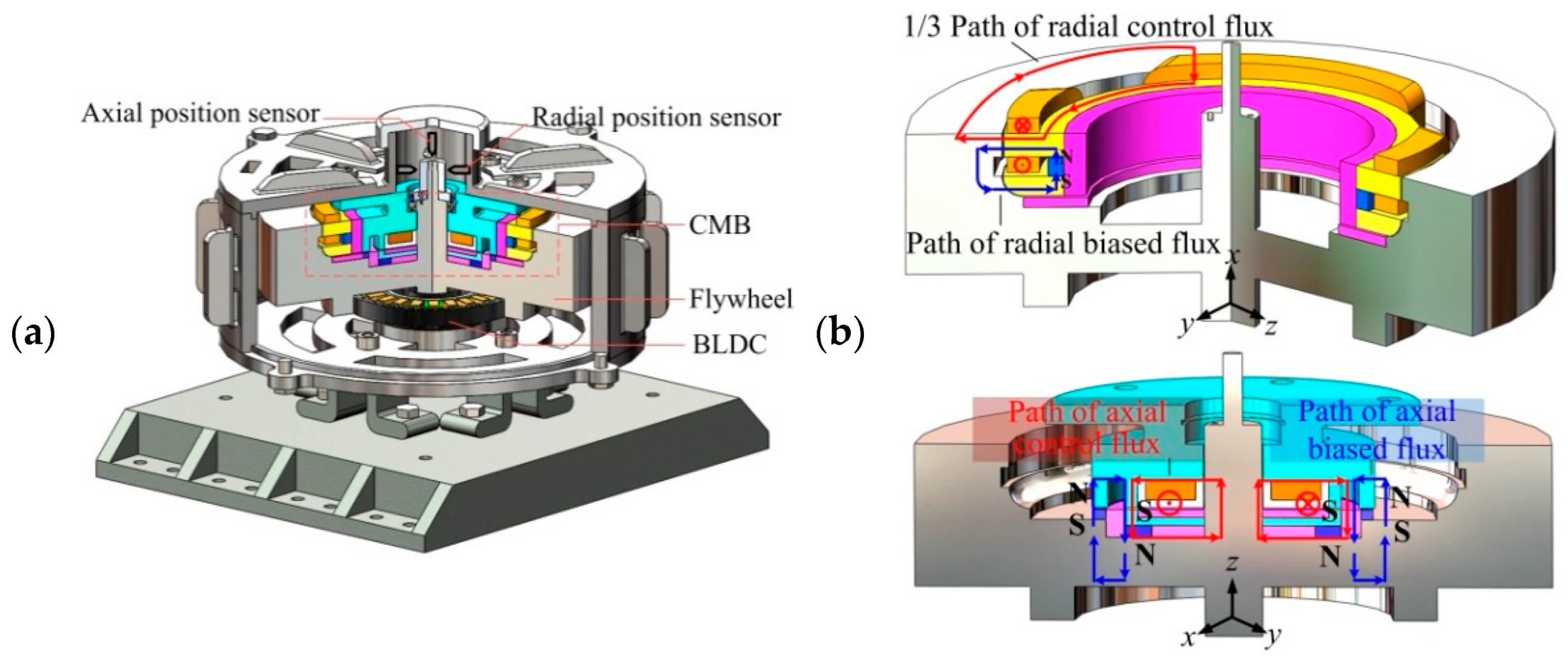
The configuration and magnetic circuits of the flywheel battery system are shown in Figure 1. As shown in Figure 1, the radial hybrid magnetic bearing (R-HMB) is used to provide radial 2-DOF stability, and the flywheel is balanced in the axial direction by the axial hybrid magnetic bearing (A-HMB). There is no coupling and interference between them. A more detailed magnetic circuit can be found in [17].

2.2. Vibration Influence Analysis

Taking a group of road condition contrast pictures, for example, the influence degree of radial and axial displacements is compared. As shown in Figure 2, by comparing the axial and radial displacement curves representing the influence of road conditions, respectively, it can be seen that the radial offset is much smaller than the axial offset in the condition of the same road and automobile suspension system conditions. In addition, similar comparison situation results also appeared in other conditions with the same working parameters. Therefore, compared with the radial direction of the magnetic suspension system of the flywheel battery, the axial direction is more susceptible to the influence of automobile suspension and road conditions.

Based on the above results, the reason is analyzed as follows: the disturbance force acting on the flywheel can be mainly divided into its own modal force and the external unbalanced force, which will cause the unstable vibration of each freedom of the flywheel. Specifically, in such configuration of the combination magnetic bearing (CMB) in this paper, the radial disturbance factors are mainly manifested as its own gyro effect and various working conditions in vehicle-mounted situations (acceleration and deceleration, turning, up and down the hill, etc.), hence, its radial equilibrium is mainly maintained by R-HMB [18,19]. The axial disturbance factors ignore the influence of the gyro effect, which is mainly manifested in various road conditions under vehicle-mounted applications (different levels of road bumps or longitudinal vibration of the car body, etc.). The axial disturbing force acting on the flywheel will cause its axial displacement vertically upward or downward from the equilibrium point; thus, the control current is adjusted online accordingly to keep the flywheel at equilibrium point.

To sum up, the modeling of this paper is mainly focused on the axial model, while the radial model can be modeled just by conventional methods under the influence of automobile suspension system and road conditions so as to ensure the control accuracy of the whole system.

3. Analytical Modeling of Axial Suspension System

Based on the above analysis, the modeling of the A-HMB system should be analyzed with emphasis, which is the premise and basis for the implementation of subsequent control strategies.

For the A-HMB, the axial suspension force acting on the flywheel rotor consists mainly of Maxwell force, thus according to the Maxwell tensor method, the relationship between the magnetic force (Maxwell force) and magnetic flux can be written as follows [20]:

$$F_m\left({\varphi }_s\right)=\frac{{\varphi }_s^2}{2{\mu }_0{S}_a}$$

(1)

where ϕ_s is the total magnetic flux, μ₀ is the permeability of the free space having value of 4π × 10⁻⁷ N/A², and S_a is the cross-sectional area of air gap.

For the A-HMB system, as shown in Figure 3, the Newtonian equation of motion can be written as:

$$m\ddot{x}=F_1+F_2-G+f$$

(2)

where m is the mass of the flywheel, x is the displacement, F₁ and F₂ are the magnetic force acting on the flywheel under different displacements, G is the gravity of the flywheel, and f is the external disturbance force acting on the flywheel.

At a certain time, when the flywheel generates a positive x displacement at the axial balance position, then the axial air gap will decrease, and the bias flux will increase accordingly; thus, the control flux needs to offset a certain amount of bias flux in order to make the flywheel return to the balance position. Conversely, the negative x displacement is generated, and the total flux in the air gap is the bias flux superposition control flux. From (1), Equation (2) of motion can be further written as:

$$m\ddot{x}=\frac{{\left({\varphi }_b-{\varphi }_c\right)}^2}{2{\mu }_0{S}_a}+\frac{{\left({\varphi }_b+{\varphi }_c\right)}^2}{2{\mu }_0{S}_a}-G+f$$

(3)

where ϕ_b is the bias flux, ϕ_c is the control flux.

For the A-HMB system in Figure 4, the biased flux and control flux at different axial displacements can be expressed as:

$${\varphi }_b=\frac{F_m{\mu }_0{S}_a}{2\left(x_0\pm x\right)},{\varphi }_b=\frac{F_m{\mu }_0{S}_a}{2\left(x_0\pm x\right)}$$

(4)

where F_m is the total magnetomotive force of axial PMs, x₀ is the axial air gap at the balance position, N is the number of axial coil turns, i_c is the incoming axial control current.

Further, (3) can be written in the form of magnetomotive force and control current as:

$$\begin{array}{ll}m\ddot{x}& =\frac{{\left(\frac{F_m{\mu }_0{S}_a}{2\left(x_0-x\right)}-\frac{{\mu }_0{S}_{a}N{i}_c}{\left(x_0-x\right)}\right)}^2}{2{\mu }_0{S}_a}+\frac{{\left(\frac{F_m{\mu }_0{S}_a}{2\left(x_0+x\right)}+\frac{{\mu }_0{S}_{a}N{i}_c}{\left(x_0+x\right)}\right)}^2}{2{\mu }_0{S}_a}-G+f\\ & =\frac{{\mu }_0{S}_a{\left(F_m-2N{i}_c\right)}^2}{8{\left(x_0-x\right)}^2}+\frac{{\mu }_0{S}_a{\left(F_m+2N{i}_c\right)}^2}{8{\left(x_0+x\right)}^2}-G+f\\ & =K\left(\frac{{\left(F_m-2N{i}_c\right)}^2}{{\left(x_0-x\right)}^2}+\frac{{\left(F_m+2N{i}_c\right)}^2}{{\left(x_0+x\right)}^2}\right)-G+f\end{array}$$

(5)

Equation (5) shows that the A-HMB system has strongly non-affine nonlinear dynamics. By choosing $x_1=x$, $x_2=\dot{x}$, and $u=i_c$, (5) can be represented as:

$$\{\begin{array}{l}{\dot{x}}_1=x_2\hfill \\ {\dot{x}}_2=f_m\left(x_1,u\right)+\xi \hfill \\ y=x_1\hfill \end{array}$$

(6)

where $f_m=\frac{K}{m}\left(\frac{{\left(F_m-2N{i}_c\right)}^2}{{\left(x_0-x_1\right)}^2}+\frac{{\left(F_m+2N{i}_c\right)}^2}{{\left(x_0+x_1\right)}^2}\right)$ and $\xi =\frac{f-G}{m}$.

For the non-affine nonlinear system of (6), the model of the time-varying affine nonlinear system using the Taylor series expanded by the nonlinear function f_m(x₁, u) with respect to u(t) around the time-varying linearized point μ can be written as:

$$\{\begin{array}{l}{\dot{x}}_1=x_2\hfill \\ {\dot{x}}_2=f_m\left(x_1,\mu \right)+g_d\left(x_1,\mu \right)\Delta u+d\left(t\right)\hfill \\ y=x_1\hfill \end{array}$$

(7)

where $\Delta u=u-\mu$, $g_d\left(x_1,\mu \right)={\frac{\partial f_m\left(x_1,u\right)}{\partial u}|}_{u=\mu }$, and $\left|d\left(t\right)\right|\le D$, which represents the unmodeled dynamics and external disturbances. μ should be as close to u as possible, which is chosen as $u\left(t-1\right)=\mu$.

Therefore, (7) can be written in the following modified form to obtain the affine nonlinear system model of the A-HMB system:

$$\{\begin{array}{l}{\dot{x}}_1=x_2\hfill \\ {\dot{x}}_2=f_n\left(x_1,\mu \right)+g_d\left(x_1,\mu \right)u+d\left(t\right)\hfill \\ y=x_1\hfill \end{array}$$

(8)

where

$$f_n\left(x_1,\mu \right)=f_m\left(x_1,\mu \right)-g_d\left(x_1,\mu \right)\mu$$

and

$$g_d\left(x_1,\mu \right)=-\frac{4NK}{m}\left(\frac{F_m-2N\mu }{{\left(x_0-x_1\right)}^2}-\frac{F_m+2N\mu }{{\left(x_0+x_1\right)}^2}\right)$$

4. Design of Adaptive SMC

Let the expected output displacement of the flywheel be represented by x_d, and the actual displacement is x, then the error is denoted as $e=x-x_d$. The sliding-mode function is designed as:

$$s=\dot{e}+ce$$

(9)

where $c>0$. Taking the derivative of (9) and plugging it in the value of (8), which can be obtained:

$$\dot{s}=f_n+g_{d}u+d\left(t\right)-{\ddot{x}}_d+c\dot{e}$$

(10)

From (10), the control law can be designed as the following:

$$u=\frac{1}{g_d}\left(-f_n+{\ddot{x}}_d-c\dot{e}-{\eta }_1\mathrm{sgn}\left(s\right)\right)$$

(11)

If f_n in the system is precisely known (i.e., g_d is known as well), the Lyapunov function is chosen as:

$$L=\frac{1}{2}{s}^2$$

(12)

Therefore,

$$\begin{array}{ll}\dot{L}& =s\dot{s}=s\left(f_n+g_{d}u+d\left(t\right)-{\ddot{x}}_d+c\dot{e}\right)\\ & =s\left(f_n+\left(-f_n+{\ddot{x}}_d-c\dot{e}-{\eta }_1\mathrm{sgn}\left(s\right)\right)+d\left(t\right)-{\ddot{x}}_d+c\dot{e}\right)\\ & =s\left(d\left(t\right)\right)-{\eta }_1\left|s\right|\end{array}$$

where η₁ shows a constant rate. Hence, by choosing ${\eta }_1\ge D$,$s\dot{s}\le 0$ is obtained ($\dot{L}=0$ when $s=0$). At this point, the closed-loop system is asymptotically stable and has superior robustness.

However, f_n in the actual system is often unknown and inaccurate. Moreover, excitation of unmodeled dynamics by symbolic functions will cause chattering, so it is necessary to use neural networks to approximate f_n.

4.1. Adaptive Control of RBF Network Approximation Based on Minimum Parameter Learning Method

In this study, an RBF neural network is used to approximate the uncertain term f_n adaptively. Its algorithm is given as:

$$h_j=\exp \left(-\frac{{\Vert x-c_j\Vert }^2}{2b_j^2}\right),j=1,\cdots ,m$$

(13)

From (13), f_n can be written as:

$$f_n={\mathit{W}}^{\mathrm{T}}\mathit{h}\left(\mathit{x}\right)+{\epsilon }_f$$

where x is the input signal of the RBF network, j represents the number of nodes in the hidden layer of the RBF network, $\mathit{h}={\left[h_1,h_2,\cdots ,h_m\right]}^{\mathrm{T}}$ is the output of the Gaussian function, W is the ideal neural network weight, ε_f is the neural network approximation error with $\left|{\epsilon }_f\right|\le {\epsilon }_N$, and f_n is the ideal output of the RBF network. Here, x is chosen as $\mathit{x}={\left[e\dot{e}\right]}^{\mathrm{T}}$. Therefore, the output of the RBF can be written as:

$${\widehat{f}}_n\left(x\right)={\widehat{\mathit{W}}}^{\mathrm{T}}\mathit{h}\left(\mathit{x}\right)$$

where h(x) represents the RBF Gaussian function.

The neural network minimum parameter learning method is adopted [21], defining $\phi ={\Vert \mathit{W}\Vert }^2$, φ is a normal number, $\widehat{\phi }$ is an estimate of φ, $\tilde{\phi }=\widehat{\phi }-\phi$. Equation (11) can be designed as:

$$u=\frac{1}{g_d}\left(-\frac{1}{2}s\widehat{\phi }{\mathit{h}}^{\mathrm{T}}\mathit{h}+{\ddot{x}}_d-c\dot{e}-{\eta }_2\mathrm{sgn}\left(s\right)-\lambda s\right)$$

(14)

where ${\widehat{f}}_n$ is the estimated value of RBF network, ${\eta }_2\ge {\epsilon }_N+D$, $\lambda >0$. It should be noted that the initial state needs to be given a preset control input; that is, the initial value of g_d is assumed to be given in order to realize the initial suspension of the system. However, this is not inconsistent with the unknown dynamic model of the whole system because the unknown factor in the axial direction is defined as the uncertain axial displacement and corresponding control current changes.

From (14), we can write (10) as that

$$\begin{array}{ll}\dot{s}& ={\mathit{W}}^{\mathrm{T}}\mathit{h}+\epsilon +\left(-\frac{1}{2}s\widehat{\phi }{\mathit{h}}^{\mathrm{T}}\mathit{h}+{\ddot{x}}_d-c\dot{e}-{\eta }_2\mathrm{sgn}\left(s\right)-\lambda s\right)+d-{\ddot{x}}_d+c\dot{e}\\ & ={\mathit{W}}^{\mathrm{T}}\mathit{h}+\epsilon -\frac{1}{2}s\widehat{\phi }{\mathit{h}}^{\mathrm{T}}\mathit{h}-{\eta }_2\mathrm{sgn}\left(s\right)+d-\lambda s\end{array}$$

4.2. Stability Analysis

The Lyapunov candidate function is chosen as:

$$L=\frac{1}{2}{s}^2+\frac{1}{2\gamma }{\tilde{\phi }}^2$$

(15)

where γ is the adaptive learning rate parameter with $\gamma >0$. In the training process of the adaptive SMC controller, the value of γ should be chosen reasonably because its value will affect the asymptotic stability and the optimal transient control performance of the system. Therefore, the derivative of L can be derived that

$$\begin{array}{ll}\dot{L}=s\dot{s}+\frac{1}{\gamma }\tilde{\phi }\dot{\widehat{\phi }}& =s\left({\mathit{W}}^{\mathrm{T}}\mathit{h}+\epsilon -\frac{1}{2}s\widehat{\phi }{\mathit{h}}^{\mathrm{T}}\mathit{h}-{\eta }_2\mathrm{sgn}\left(s\right)+d-\lambda s\right)+\frac{1}{\gamma }\tilde{\phi }\dot{\widehat{\phi }}\\ & \le \frac{1}{2}{s}^2\phi {\mathit{h}}^{\mathrm{T}}\mathit{h}+\frac{1}{2}-\frac{1}{2}{s}^2\widehat{\phi }{\mathit{h}}^{\mathrm{T}}\mathit{h}+\left(\epsilon +d\right)s-{\eta }_2\left|s\right|+\frac{1}{\gamma }\tilde{\phi }\dot{\widehat{\phi }}-\lambda s^2\\ & =\tilde{\phi }\left(-\frac{1}{2}{s}^2{\mathit{h}}^{\mathrm{T}}\mathit{h}+\frac{1}{\gamma }\dot{\widehat{\phi }}\right)+\frac{1}{2}+\left(\epsilon +d\right)s-{\eta }_2\left|s\right|-\lambda s^2\\ & \le \tilde{\phi }\left(-\frac{1}{2}{s}^2{\mathit{h}}^{\mathrm{T}}\mathit{h}+\frac{1}{\gamma }\dot{\widehat{\phi }}\right)+\frac{1}{2}-\lambda s^2\end{array}$$

The adaptive law for tuning the weight in order to approximate the function ${\widehat{f}}_n\left(x\right)$ is designed as

$$\dot{\widehat{\phi }}=\frac{1}{2}\gamma s^2{\mathit{h}}^{\mathrm{T}}\mathit{h}-k\gamma \widehat{\phi }$$

(16)

where $k>0$. Hence, it can be further obtained as

$$\begin{array}{ll}\dot{L}& \le -k\tilde{\phi }\widehat{\phi }+\frac{1}{2}-\lambda s^2\le -\frac{k}{2}\left({\tilde{\phi }}^2-{\phi }^2\right)+\frac{1}{2}-\lambda s^2\\ & =-\frac{k}{2}{\tilde{\phi }}^2-\lambda s^2+\left(\frac{k}{2}{\phi }^2+\frac{1}{2}\right)\end{array}$$

Taking $k=2\lambda /\gamma$, then

$$\begin{array}{ll}\dot{L}& \le -\frac{\lambda }{\gamma }{\tilde{\phi }}^2-\lambda s^2+\left(\frac{k}{2}{\phi }^2+\frac{1}{2}\right)\\ & =-2\lambda \left(\frac{1}{2}{s}^2+\frac{1}{2\gamma }{\tilde{\phi }}^2\right)+\left(\frac{k}{2}{\phi }^2+\frac{1}{2}\right)=-2\lambda L+R\end{array}$$

where $R=\frac{k}{2}{\phi }^2+\frac{1}{2}$. Solving the above inequality can get

$$L\le \frac{R}{2\lambda }+\left(L\left(0\right)-\frac{R}{2\lambda }\right)e^{-2\lambda t}$$

Hence,

$$\underset{t\to \infty }{\lim }L=\frac{R}{2\lambda }=\frac{\frac{k}{2}{\phi }^2+\frac{1}{2}}{2\lambda }=\frac{\frac{2\lambda }{\gamma }{\phi }^2+1}{4\lambda }=\frac{{\phi }^2}{2\gamma }+\frac{1}{4\lambda }$$

Therefore, by choosing $0<R\le \left|-2\lambda L\right|$, the result $\dot{L}\le 0$ is obtained. Among them, if $s\ne 0$, then $\dot{L}<0$, if $s=0$, then $\dot{L}\equiv 0$. Meanwhile, due to $L\ge 0$ and the control input u is bounded by the maximum value of u_m, i.e., $u\le u_m$, so the s and $\tilde{\phi }$ are uniformly bounded. According to the LaSalle invariance principle on the basis of the Lyapunov stability discriminant generalization theorem, the closed loop system is asymptotically stable, when $t\to \infty$, then $s\to 0$, and thus, $e\to 0$, $\dot{e}\to 0$. 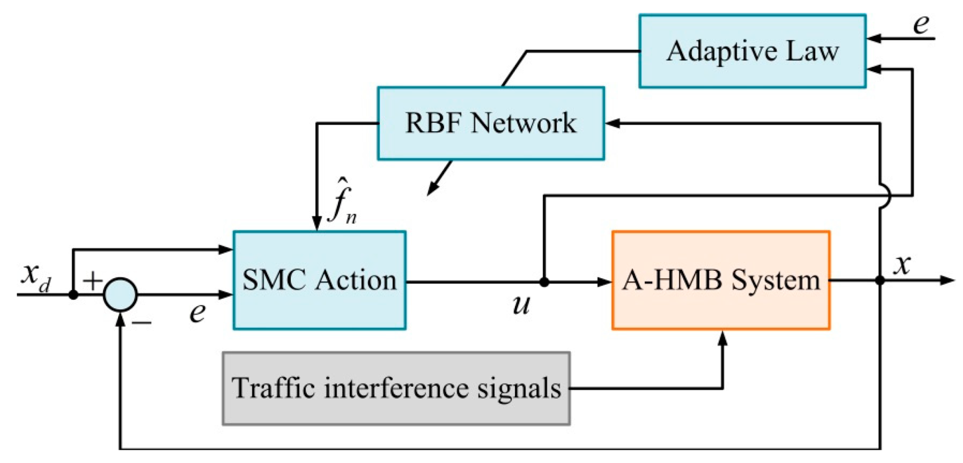Finally, the objective of function approximation can be realized. The overall control scheme block diagram of the control system is shown in Figure 4.

5. Simulation Results and Analysis

By using the designed SMC and the nonlinear analytical model of A-HMB, a simulation is executed using similar design parameter values as of the prototype system to verify the performance of the controller. Mass of the flywheel is 2.8 kg, the initial balance position of the flywheel is set to 0.5 mm according to the axial air gap, magnetic force constant K is 7.5 × 10⁻¹¹, the magnetomotive force of axial PMs is about 150 AT, and the number of axial coil turns is 250.

RBF network is chosen by a two input-five hidden-one output, and the initial weight value of RBF is set to 2. The value of c_j is 0.5, and b_j is 5. The control law and adaptive law are designed using (14) and (16), respectively; the value of the parameter is λ = 40, and the adaptive learning rate parameter is γ = 150. In the sliding function, the values of the parameters set as c = 200, η₂ = 30 according to the results of multiple debugging. The output response begins to oscillate above the value of γ, and hence, these optimal values are selected for the adaptive learning parameter to give the best transient response.

5.1. Interference Analysis of Road Roughness

Different from the traditional study of road condition representations, the interference signals of different road conditions are considered as unmodeled dynamics in the control system is one of the important innovations of this paper. The schematic diagram of the vehicle driving on the road is shown in Figure 5. In general, the road surface is uneven, and the description of the road roughness (Considering the most common cases, the time-domain model of pavement in the form of filtered white noise is mainly considered) can be expressed [22,23]:

$${\dot{z}}_g\left(t\right)=-2\pi n_{1}u{z}_g\left(t\right)+2\pi n_0\sqrt{G_q\left(n_0\right)u}\cdot \varpi \left(t\right)$$

(17)

where z_g is the displacement of the road roughness, n₀ is the reference spatial frequency, which is generally taken as 0.1 m⁻¹; n₁ is the cut-off space frequency under road roughness, which is taken as 0.01 m⁻¹, i.e., the corresponding maximum road surface wavelength is 100 m; G_q(n₀) is the roughness coefficient of road surface, its geometric average value is determined according to the grade of different road roughness; u is the speed of the vehicle, ϖ(t) is the Gaussian white noise signal, which is related to the amplitude of power spectral density and sampling frequency.

The disturbance excitation of different road levels is only aimed at the A-HMB system, and the vehicle suspension system is not taken into consideration. Road excitation produces vibration in the vertical direction (z-axis) of the vehicle and is then transferred to the flywheel system to affect its axial stability. In the simulation process, the initial state of the flywheel is in the axial balance position; that is, there is no output displacement under ideal circumstances, and then the ideal output displacement is assumed to fluctuate sinusoidally within the allowable range of 0.05 mm. It is assumed that the vehicle travels at a constant speed of u = 30 m/s (the same goes for speed changes). The amplitude of power spectral density and sampling frequency of all white noise signals under interference are uniformly set at 0.5 and 10 Hz. When the SMC is involved, the tracking of the axial output displacement and response velocity of the flywheel is observed.

5.2. Results Analysis

In order to verify the effectiveness of the proposed control law, the analyses of the results are as follows. Figure 6a shows the plots for f_n and ${\widehat{f}}_n$ with non-interference signal. Taking C-grade road surface as an example, Figure 6b shows its plots for f_n and ${\widehat{f}}_n$. The more intense the external interference, the less accurate the system approximates f_n.

The control current input of the system is shown in Figure 7. Figure 7a shows the axial control current input without interference, which changes correspondingly with the stable displacement of the system, and its average value remains around 1.5 A. As shown in Figure 7b, a disturbance of the C-level road surface is added to the system model as unmodeled dynamics by this time. It can be seen that under the influence of the control law, the control current (control input signal) is indeed adjusted in real time to maintain the axial stability of the system. It can be seen that with the aggravation of bad road conditions, the control current changes greatly under the influence of the control law of the system, which aims to make the system have enough robustness after rapid adaptive adjustment.

Furthermore, it is very important to verify the robust performance of the controller more widely and comprehensively. The indexes to evaluate robust performance include dynamic performance such as signal tracking, interference suppression, and real-time responsiveness. Figure 8 shows the corresponding displacement and response speed of the A-HMB system generated by the non-interference signal and the interference signals with different road roughness levels as the unmodeled dynamics. It can be seen that, when there is no interference, the system shows great tracking performance under the action of adaptive SMC and can adjust accordingly with the expected output displacement in real time. Even under the influence of different road surface roughness, the overall fluctuation error is within the acceptable permissible range, and the adaptive tracking advantage is still significant.

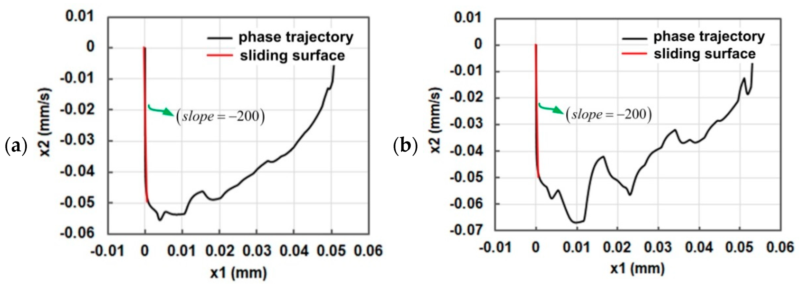
Figure 9a,b show the phase trajectory when A-level road surface and C-level road surface is included in the system as unmodeled dynamics, respectively. It can be seen that both trajectories slide along the preset sliding surface c, which has an absolute slope of 200. Therefore, it can be seen that even under the interference of road conditions, the designed SMC can still make the system state slide along the sliding mode surface with a fast response speed, and the chattering phenomenon is well solved.

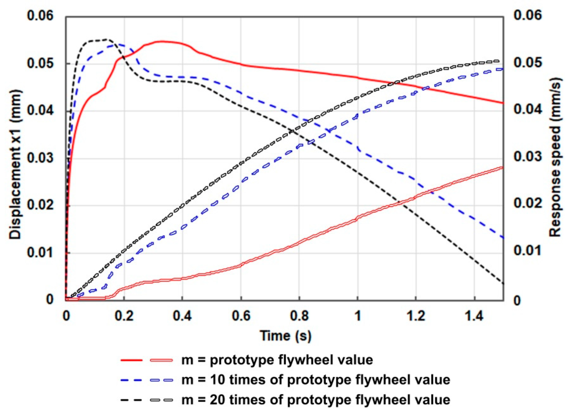
To further verify the advantages of a robust controller, the physical parameters of the AMB system (taking the flywheel mass as an example) are varied from 10 to 20 times the prototype value. The reason to expand the mass as a verification index is that the flywheel of the prototype system in this paper is only experimental, while the actual flywheel mass is much greater than this. The simulated output response of the A-HMB system should remain bounded for the variation in parameters.

Figure 10 shows the output response with flywheel mass 10 times and 20 times the prototype value. As shown in Figure 10, it can be shown that the simulated output response of the A-HMB is indeed bounded, so its tracking performance is very good; that is, its robustness is still very good.

Further, the performance of the proposed robust controller is compared with that of the classical PID controller. According to (2), ignoring the external disturbance force, the open-loop transfer function of the system can be approximated as a second-order oscillation link G(s) = k_izc/(ms²-k_x) (where k_izc is the axial current stiffness and k_x is the axial displacement stiffness) through the Laplace transform [24]. The parameters of the PID controller for the A-HMB are K_p = 2, K_i = 0.1 and K_d = 30.

Figure 11 shows the comparison results between the PID controller and the SMC for the position tracking of the A-HMB system under discrete sinusoidal signals. From Figure 11, it can be seen that SMC can achieve better global tracking performance from the beginning to the end compared with the intact local tracking performance under the control of the traditional PID controller. Therefore, on the whole, SMC has significantly better robustness than the traditional PID controller.

6. Experimental Results and Analysis

To verify the control performance of the proposed SMC under the influence of road conditions, an experimental platform is set up for evaluation. It should be noted that the radial suspension control of the prototype still uses the classical linear PID controller because the radial air gap of R-HMB is always in the linear range. In short, when the radial perturbation occurs, the R-HMB system is regarded as a linear system. On the contrary, when axially disturbed, the A-HMB system is regarded as a time-varying nonlinear system (the axial air gap is 0.5 mm, which exceeds the linear air gap of 0.25 mm). The specific radial and axial disturbance factors are analyzed in Section 2.

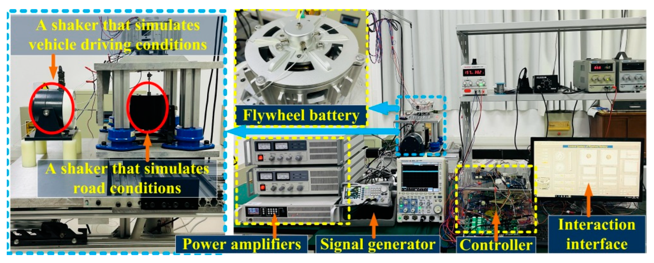
The overall experimental platform is shown in Figure 12. It mainly includes a prototype body of the vehicular flywheel battery, an operating platform used for simulation of different working states and a set of the controller.

The principle of the experimental device to simulate road conditions is as follows: The signal generator sends a signal simulating the road condition excitation, and then the signal is amplified and output by the power amplifier to drive the shaker. Therefore, the push rod of the shaker will impact the base of the flywheel battery according to the frequency of the road condition signal so as to realize the performance test experiment simulating the influence of the vehicle flywheel battery by the road condition disturbance. It should be noted that since the road noise signal is converted into a force signal and transmitted to the system, the feedback mechanism of the actual control system is still the feedback of displacement, and the error derivative of the system input signal is operable under the measurement noise.

During the experiment, the working speed of the flywheel is maintained at 1500 r/min, and its purpose is to weaken or even strip out the gyroscopic effect caused by high-speed flywheel battery and purely analyze the robustness of the flywheel battery system due to road disturbance. The path spectrum frequency applied to the signal generator is set at 4 Hz, and its amplitude varied according to different levels of road conditions. Here, one thing to be clear is that the road spectrum amplitude set has taken the speed of the vehicle into account (Equation (17)) so as to avoid the defect that the experiment cannot simulate the actual constant speed.

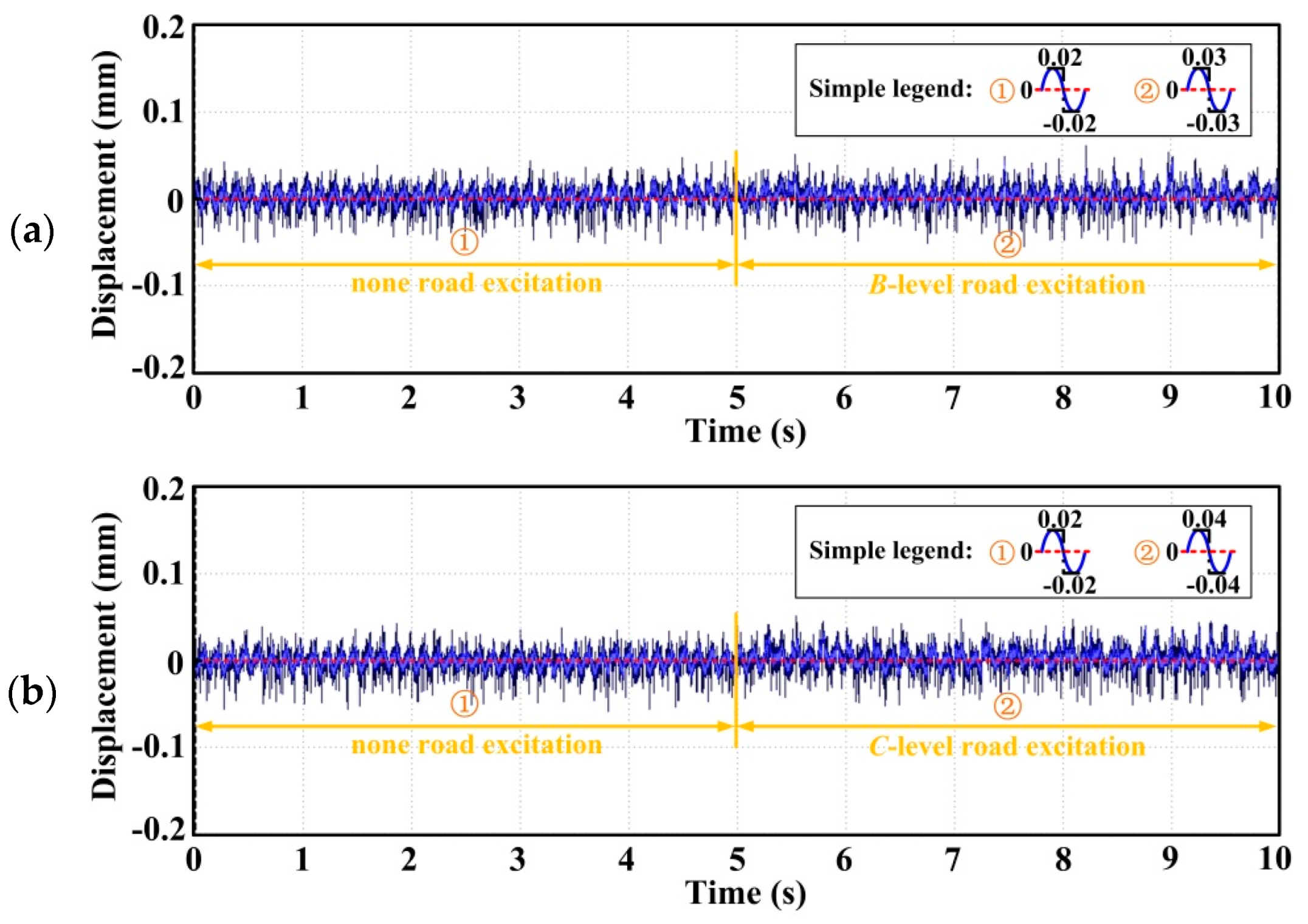
Figure 13a shows the change of axial displacement of the flywheel from static suspension (no external excitation) to the application of B-level road excitation. Similarly, the change of that with C-level road excitation is shown in Figure 13b. As can be seen from Figure 13, when the flywheel is suspended in an axial static state, the fluctuation range of its displacement is maintained at ±0.02 mm. At this time, under the interference of B-level and C-level road surface, the fluctuation of its axial displacement increases by ±0.01 mm and ± 0.02 mm, respectively, but the overall displacement trend still follows the state of normal suspension within the preset ideal displacement controllable range (±0.05 mm). Therefore, the proposed SMC has great performance, and it is proven to have good robustness.

Figure 14 shows the axial displacement of the flywheel under the interference of sustained B-level and C-level road conditions. It can be seen that, under sustained road excitation, the axial displacement always follows the preset ideal displacement trajectory and maintains a good continuity, which indicates that the proposed SMC has a fast response speed. Therefore, the good robustness is further proved by the experimental results.

7. Conclusions

In this paper, taking the magnetic suspension control system of a vehicle-mounted flywheel battery as an example, a robust controller (SMC) considering the interference of road surface roughness is proposed. Moreover, the controller is established according to the simulation signals of road conditions rather than the imaginary random type signals. Therefore, the algorithm in this paper has strong reliability and practical significance. Various simulations of the control law and considering the robustness performance are skillfully performed and analyzed, which demonstrate the superiority of the proposed controller. In addition, because the existing methods are too complicated to construct an adaptive law, which affects the real-time performance, in our study, the weight adjustment of the traditional neural network is replaced by the designed adaptive law of parameter estimation, which enhances the real-time performance of the system and is beneficial to the engineering application. Moreover, the experimental platform simulating the road condition is cleverly designed, which is the first ingenious use of signal generators, shakers, power amplifiers, etc., to simulate the excitation of the road condition (based on the road condition spectrum), so it can be used to verify the correctness of the control strategy proposed in this paper. Good experimental results show that the controller has good robustness under different road conditions.

In addition, it is worth noting that the robust controller is only designed for the disturbance considering the influence of road conditions, but not the driving conditions. In order to further improve the robustness and stability of the flywheel battery system, a composite controller accounting for vehicle driving and road conditions should be further considered. Moreover, a vehicular flywheel battery experiment platform based on mobile vehicles should be designed in the future to verify the feasibility of the proposed controller. With the help of the experimental platform of mobile vehicles, more comprehensive experiments can be done combining various vehicle and road conditions that are closer to the actual situations. The experimental tests such as crossing the isolation zone, acceleration, deceleration, uphill, downhill, and turning on different roads can be conducted, which can verify or further improve the proposed controller.