Experimental Investigation of the Steady-State Flow Field with Particle Image Velocimetry on a Nozzle Check Valve and Its Dynamic Behaviour on the Pipeline System

Abstract

In the present work, to investigate the hydraulic losses and safe operation of nozzle check valves in industrial piping systems, the static characteristics of the valve and its dynamic behavior in the pipeline system were studied using an experimental bench with a visual DN300 nozzle check valve. Besides, basing on the PIV (Particle Image Velocimetry) technique measures the valve steady-state flow field under the different flow rates. The study has shown that as the flow rate rises, the valve disc displacement slowly increases to 44 mm, then rapidly increases to a maximum displacement of 72 mm. When the Reynolds number exceeds 5 × 10⁵, the relationship between pressure drop and flow obeys a quadratic function. The local vortex area formed by the flow passage near the downstream deflector expands with the flow improvement. As the increase of flowrate, at low flow operating conditions, the downstream flow velocity in the local high-speed area near the valve body increases; at medium operating conditions, the area’s flow velocity decreases; at high flow work, this local high-speed area disappears. When the fluid deceleration is lower than 4 m/s², the dynamic behavior satisfies the quadratic curve when the maximum slope is only 0.354, which shows that this nozzle check valve has a favorable response to the system.

1. Introduction

As the main component of the pump system, the check valve has a simple and compact structure and is easy to install and maintain. When the pump stops running, the check valve can effectively prevent the reversal of the impeller caused by the backflow of the fluid, which significantly lowers the risk of damage to the equipment and plays a critical role in the safe operation of the entire pump system. The evaluation criteria of the check valve mainly include two points. First, when the valve is in ordinary operating (open state), it is desired that the pressure loss is lower. The pressure loss feature of the check valve in general operation belongs to its static characteristics. Second, when the valve is suddenly closed, there is the desire to generate the lowest possible water hammer pressure. The dynamic response between the valve pressure and the system pressure caused by closing the valve belongs to its dynamic characteristics. Compared with other structural types of check valves, the nozzle check valve has better static and dynamic characteristics. The study of the static and dynamic characteristics of the nozzle check valve has considerable guiding significance for the optimal design of the valve.

With the development of computational fluid dynamics (CFD), related scholars have used the RNG (Renormalization Group) k-ε turbulence model to calculate the pressure drop and flow coefficient of the steady flow of nozzle check valves with different openings [1]. This method can also calculate unsteady flow within the valve during valve opening [2]. The researchers found that flow separation created in the valve downstream keeps a period after the valve opened, which results in an additional increase of the pressure drop in the upper half travel of the disc, the pressure drop deviating from the quasi-steady-state characteristic curve of the valve [3]. The spring preload and stiffness significantly influence the characteristics of the check valve. In low flow, when the spring force exceeds the maximum hydrodynamic force, the valve disc does not open completely, causing the internal parts of the valve to vibrate, and repeatedly high-speed impact, the check valve self-destructs. When designing a nozzle check valve, considering the relationship between the flow characteristics of the valve in the fully open position and the performance curve of the working machine selects the spring preload and stiffness [4]. The upstream flow velocity also affects the performance of the check valve. The disc does not move until the flow rate increases to a fixed value, and a local peak occurs in pressure drop. As the flow rate gradually rises, the disc opening and the pressure drop increase. The pressure drop rapidly grows when the disc opening reaches its maximum [5]. The dynamic interaction between the check valve disc and the fluid forms a complex and variable flow field, whereas the hydraulic force on the disc is uncertain. Guohua Li and Jim C. P. Liou pointed out that the hydraulic torque of the swing check valve can classify into the torque caused by the flow around the stationary disc and the torque generated by the rotation of the disc [6].

PIV (Particle Image Velocimetry) measurement hardly disturbs the flow field, and its measurement results are closer to the actual flow. In recent years, the development of PIV technology has given a great impetus to the measurement of the internal flow field of fluid machinery [7,8,9,10,11]. CFD simulations require simplified processing of geometric models, boundary conditions, and calculation methods, resulting in some non-negligible errors between the calculated results and the PIV measurement results. Therefore, there is a critical need for PIV techniques to study the flow characteristics of nozzle check valves.

Regarding the dynamic behavior of check valves, as early as 1980, G. A. Provoost conducted an experimental study on two kinds of check valves (ball and pendulum) and suggested that the value of the gradient of fluid velocity with time is crucial when studying the dynamic characteristics of check valves [12]. By 1989, A. R. D. Thorley proposed the theory of dimensionless dynamic behavior of check valves. He argued that the maximum acceptable reverse flow velocity through the valve could be a control parameter in valve calculation procedures. In addition, the average deceleration of the fluid provided an essential link to the selection of the most suitable check valve [13]. Thus, the check valve dynamic characteristics effectively interconnect the piping system and the valve. For example, the maximum slope of the dynamic characteristic curve of a check valve installed in a centrifugal compressor circulation system determines the maximum tolerance that the compressor/recirculation system allows backflow through the valve [14]. To effectively prevent water hammer in the piping system can be guided by the check valve dynamic characteristics to take some measures. In the pump-pressurized primary system with an air tank, when the transient circulation system generates the negative water hammer pressure, the outflow throttling from the air container can minimize the check valve “slam” [15]. In the experimental circuit of a nuclear power plant, the reverse check valve under reverse flow pressure difference can effectively suppress the water hammer phenomenon during the transition of parallel double pump switching [16].

For the dynamic characteristics of check valves, related scholars have also studied the dynamic closing process of check valves by the CFD technique, mainly including the dynamic mesh method and overlapping mesh method. Nam-Seok Kim and Yong-Hoon Jeong performed CFD calculations of the closing process of a swing check valve using four dynamical mesh techniques. The results showed that the velocity distribution at the valve outlet of each method was similar before the valve disc was almost closed. However, the inflowing fluid velocity prediction varied when the valve was fully closed [17]. Zhounian Lai et al. applied the overlapping grid technique to CFD calculations of a double-disc check valve to achieve complete closure and accurately capture pressure fluctuations. He illustrated the effects of system outlet pressure, initial flow rate, and upstream pump shutdown speed on pressure fluctuations caused by check valve closure [5].

In the current research on the static characteristics of check valves, related academics mainly use the CFD method to calculate the internal flow field or measure the relationship between pressure drop and flow rate through experiments. There are few studies on measuring the internal flow field of check valves. However, the valve disc is static during regular operation of the valve. The internal flow field significantly influences the static characteristics, which has a guiding value for the optimal design of check valves. The dynamic behavior is the process of the check valve dynamically responding to the system. The current CFD technology cannot accurately calculate the dynamic characteristics [18,19,20], so most scholars still use the experimental method. It has been a dilemma to measure the maximum reverse flow velocity by electromagnetic flowmeter because the time of backflow formed in the check valve is exceedingly short, which is a challenge for the dynamic characteristics experiment of the check valve [21,22,23]. In this study, using the PIV technique measures the steady-state flow field of the valve under the different flow rates on a constructed suitable experimental bench. In addition, using the method of testing the pressure surge obtains the maximum reverse flow velocity and further derives the dynamic characteristics of the valve. This paper can provide a favorable reference for the design of other nozzle check valves.

2. Experimental Setup

2.1. Experimental Aims and Methods

Figure 1 shows the structure diagram of the nozzle check valve (fully open), which mainly includes the valve body, valve disc, upstream deflector, downstream deflector, spring, and other components. When the upstream fluid acts on the valve disc, the valve disc compresses the spring and opens. Upstream pressure is less than the spring force, and the valve disc begins to close. The downstream pressure is higher than the upstream pressure. The valve closes to form a short period of reverse flow until the valve disc is fully closed, the reverse flow stops, and the downstream produces a water hammer.

In this study, firstly, the pressure drop and the opening degree of the check valve are measured at different flow rates during its regular operating to explore their relationship with flow rate, further obtaining the valve flow resistance characteristics. Then, the PIV technique is applied to obtain the flow field characteristics inside the valve at different flow rates. Finally, artificially creating the valve closing abruptly, the transient change in pressure upstream and downstream of the closing process is measured, thus obtaining the response relationship between the valve and the system.

2.2. Experimental Principles

2.2.1. Principle of PIV Flow Velocity Measurement

The PIV is a technique for measuring the flow field non-perturbatively [24,25,26,27,28]. Tracer particles with comparable density with the fluid can uniformly disperse in the fluid, with excellent followability and higher reflectivity. Two images of the tracer particles (frame A and frame B) were taken before and after the Δt time interval using a CCD camera. Using a cross-correlation algorithm to process the two images obtains the relative positions of each tracer particle before and after the Δt time interval. Both x(t) and y(t), the displacement in the x and y directions, is a function of time t. This tracer particle flow velocity can express as (1):

$$\{\begin{array}{l}{v}_{\mathrm{x}}=\frac{\mathrm{d}x\left(t\right)}{\mathrm{d}t}\approx \frac{\mathsf{\Delta }x}{\mathsf{\Delta }t}={\overline{v}}_{\mathrm{x}}\\ v_{\mathrm{y}}=\frac{\mathrm{d}y\left(t\right)}{\mathrm{d}t}\approx \frac{\mathsf{\Delta }y}{\mathsf{\Delta }t}={\overline{v}}_{\mathrm{y}}\end{array}$$

(1)

where ν_x and ν_y are the instantaneous velocities of the tracer particles along with the x and y directions, and ${\overline{v}}_{\mathrm{x}}$, ${\overline{v}}_{\mathrm{y}}$ are the average velocities of the fluid masses along the x and y directions. Δx and Δy are the displacements of tracer particles in x and y direction, respectively. In (1), when Δt is small enough, the magnitudes of ν_x and ν_y can reflect ${\overline{v}}_{\mathrm{x}}$, ${\overline{v}}_{\mathrm{y}}$.

The cross-correlation algorithm can determine the displacement of tracer particles by querying and matching the light intensity information reflected from the tracer particles in two images when the light intensity information of the two images is the same.

$$g_2(x,y)=g_1(x-\mathsf{\Delta }x,y-\mathsf{\Delta }y)$$

(2)

where, g₁ and g₂ is the light intensity function reflected by the tracer particle in image (frame A and frame B), respectively.

Applying the Fourier transform to Equation (2), it can be obtained to Equation (3).

$$G_2(u,v)=G_1(u,v)e^{-2\pi i(u\mathsf{\Delta }x+v\mathsf{\Delta }y)}$$

(3)

Define R_ccf as the cross-correlation function of g₁ and g_2.

$$R_{ccf}(x,y)=g_1(x,y)\ast g_2(-x,-y)$$

(4)

Applying the Fourier transform to Equation (4) and according to the convolution theorem, it can be obtained to Equation (5).

$$R_{ccf}(u,v)=G_1(u,v)G_2^{*}(u,v)=G_1{G}_1^{*}{e}^{2\pi i(u\mathsf{\Delta }x+v\mathsf{\Delta }y)}=F(u,v)e^{2\pi i(u\mathsf{\Delta }x+v\mathsf{\Delta }y)}$$

(5)

where, $F(u,v)=G_1{G}_1^{*}$.

Carrying out Fourier inverse transform to Equation (5), it can be obtained to Equation (6).

$$R(x,y)=F(x,y)\ast \delta (x-\mathsf{\Delta }x,y-\mathsf{\Delta }y)=F(x-\mathsf{\Delta }x,y-\mathsf{\Delta }y)$$

(6)

According to the autocorrelation function’s characteristic, function F(x, y)’s peak point is at the original point, so the peak point of function R(x, y) is at (Δx, Δy). The image pairs are gridded, and the computer calculates the extreme values of the interrelation function of the image pairs. The position of the extreme values determines the displacement of the tracer particle at time interval Δt. Hence, Equation (1) enables us to obtain the distribution inside the flow field.

Figure 2 shows a diagram of the PIV flow velocity measuring system. The accuracy of 1% PIV can measure the flow velocity range of 0–800 m/s, which processing software is Insight 4G. The laser emitter is an Nd-YAG double pulse laser, model Vlite-380, with a single pulse energy of 380 mJ, an operating wavelength of 532 nm, and a maximum repetition frequency of 15 Hz. The camera was an Imager Pro X 4M CCD camera, model 630090-ST, with a minimum interval of 115 ns for double span frames, a resolution of 2048 × 2048, and a frame rate of 16 fps. The tracer particles are V3V hollow glass seed particles, model 10090, with a particle diameter of 55 µm.

First, the laser beam from the pulsed laser emitter is refracted into a light sheet when it strikes a cylindrical mirror. The laser sheet is directed parallel to one axial plane of the nozzle check valve and illuminates the tracer particles on the axes. Then, the CCD camera takes the images of the illuminated tracer particles. In this process, it is necessary to set the signal sequences in the computer. The synchronizer controls the time sequence, where the laser emitter with a double pulse laser and the CCD camera with double span frames. For each pulse signal, only laser A lights up the tracer particles for the first exposure. Only the laser B lights up the tracer particles for the second exposure and ensures that the laser emission time interval is Δt. The CCD camera transmits each pair of images taken to the computer. The image pairs are cross-correlatively calculated in the computer to obtain multiple sets of flow field velocity vectors. The velocity vectors of each group are averagely calculated to enhance the accuracy of the flow field and achieve the average velocity distribution of the steady-state flow field.

2.2.2. Principle of Dynamic Characteristics Testing

The dynamic characteristics of the check valve are the relationship between the fluid deceleration of the piping system and the maximum reverse flow velocity through the check valve. The fluid decelerating is the change rate of the average flow velocity dv/dt when the flow velocity decreases from a stable value to zero in the closing of the check valve.

$$\mathrm{d}v/\mathrm{d}t=\mid \frac{0-v_0}{t_{\mathrm{d}}}\mid =\frac{v_0}{t_{\mathrm{d}}}=\frac{4Q_0}{\pi t_{\mathrm{d}}{d}^2}$$

(7)

where, v₀ is the average fluid velocity of steady flow; Q₀ is the flow rate of steady flow; t_d is the time for the fluid velocity to reduce from v₀ to zero; d is the diameter of the coupling pipe downstream of the valve, which is 0.3 m in this study.

During the closing of the check valve, the upstream pressure continues to decrease, and the fluid undergoes instantaneous reverse flow until the check valve is completely closed and the reverse flow stops, generating a water hammer. This value of water hammer pressurization caused by changes in flow velocity in a straight pipe satisfies the Joukousky equation [29,30].

$$\mathsf{\Delta }H=-\frac{a\mathsf{\Delta }v}{g}$$

(8)

$$\mathsf{\Delta }p=\rho g\mathsf{\Delta }H=-\rho a\mathsf{\Delta }v$$

(9)

where, Δp is the water hammer pressurization; Δv is the change in fluid velocity; ρ is the fluid density; g is the acceleration of gravity, taking 9.81 m/s²; a is the water hammer wave speed, when the ratio of pipe diameter (300 mm) to pipe wall thickness (3 mm) is 100, taken as 1000 m/s in the steel pipe [30].

After the downstream pipe reaches the maximum reverse flow velocity v_R, the backflow stops abruptly and its velocity changes as:

$$\mathsf{\Delta }v=0-v_{\mathrm{R}}$$

(10)

From Equations (8) and (9), it is obtained that:

$$v_{\mathrm{R}}=\frac{\mathsf{\Delta }P}{\rho a}$$

(11)

The check valve’s dynamic characteristics test measures the flow rate of steady flow Q₀, fluid deceleration time t_d, and pipe diameter d. Using Equation (7) can calculate the deceleration of the fluid dv/dt. Due to the brief duration of backflow, it is not easy to accurately measure the maximum reverse flow velocity v_R using the electromagnetic flowmeter. In this study, as shown in Equation (11), the measured water hammer surge Δp can be used to calculate the maximum backflow velocity v_R. Adjusting the flow rate Q₀ and deceleration time t_d obtains different pairs of numbers (dv/dt, v_R). Adopting the fluid deceleration dv/dt as the horizontal axis, the maximum reverse velocity v_R as the vertical axis, the check valve dynamic characteristics curve can be plotted.

2.3. Experimental System and Process

Figure 3 shows the testing system of the nozzle check valve. The main components include high pool A1, low pool A2, centrifugal pump CP, pressure transducers (P1, P2), electromagnetic flow meter EF, throttle valve THV, controlling valves (CV1-CV4), tested nozzle check valve TV, PIV test system, LMS data acquisition system.

Table 1. Parameters of the key experimental instruments.

Experimental Instruments	Parameters	Values
High water pool	Volume	24 m3
	Height from the tested valve	20 m
Centrifugal pump	Rated head	40 m
	Rated flowrate	684 m3/h
Pressure sensor	Range	−0.1–1.5 MPa
	Accuracy	0.25%
Electromagnetic flowmeter	Specification	DN300
	Range	0–1000 m3/h
	Accuracy	0.21%
LMS data acquisition system	Sampling frequency	6400 Hz
	Digital-to-analog conversion	24 bits
PIV particle image velocimetry system	Pulse frequency	15 Hz
	Exposure duration	400 µs
	The time interval	350 µs

presents the relevant parameters of the main instruments. In Figure 3, the cyan arrow indicates the direction of flow driven by gravity, and the red arrow indicates the direction of flow powered by a centrifugal pump. The experiment on the static characteristics of the nozzle check valve is mainly to test the valve disc displacement, pressure drop, and flow field distribution at different flow rates. Figure 4 shows the flow chart of the static characteristics test. In the experiment of the dynamic characteristic, improving the downstream pressure forces the stable operating check valve to close, and the transient changes of the upstream and downstream pressure during the valve closing process are mainly measured. Figure 5 shows the flow chart testing the dynamic behavior. Figure 6 displays a physical view of this test system in the field. Figure 7 presents images of a flow passage with tracer particles taken by a CCD camera.

3. Results and Discussion

3.1. Nozzle Check Valve Static Characteristics and Flow Field Analysis

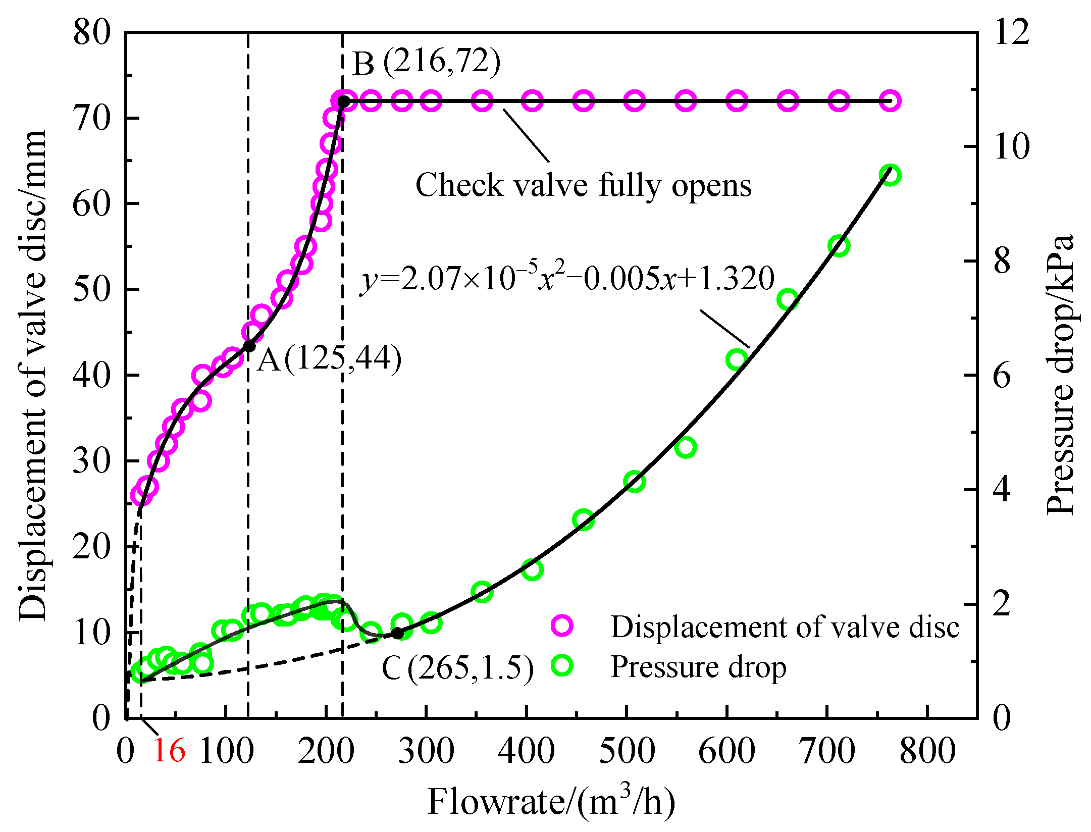
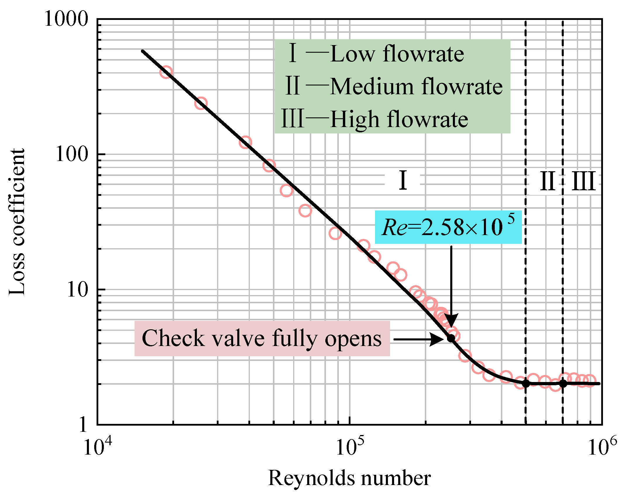
3.1.1. Static Characteristics Analysis

The valve disc displacement and upstream and downstream pressure drops vary at different flow rates during the nozzle check valve regularly operating. Figure 8 shows the relationship between valve disc displacement and pressure drop with flow rate. As can be seen, the flow rate rises to 16 m³/h, the valve disc displacement increases instantaneously from zero to 26 mm, and the pressure drop is 0.8 kPa (the minimum pressure drop of opening the valve). Due to the flow rate of less than 16 m³/h, the upstream pressure of the valve disc cannot overcome the spring preload force, which makes opening the valve disc hard.

When the flow rate is lower than 125 m³/h, the valve disc displacement increases slowly with the increase in flow rate. When it reaches 125 m³/h, the disc displacement is 44 mm (point A), it then keeps increasing the flow rate, thus, the disc displacement enhances rapidly. When the flow rate reaches 216 m³/h (the minimum flow rate of a fully opening check valve), the disc displacement reaches the maximum displacement of 72 mm (point B). It then improves the flow rate, but valve disc displacement remains constant.

This phenomenon can be explained as follows. When the valve disc displacement is less than 44 mm, the disc area impacted by the mainstream is small. When the flow rate increases, the impact force acting on the disc rises slowly, which is lower than the increase of the spring force, and the disc displacement enhances slightly. However, its displacement is greater than 44 mm, the flow passage expands, and its area is impacted by the mainstream enlarges. The impact force increases rapidly as the flow rate grows, which is higher than the increase in spring force, and the disc displacement rockets speedily to the maximum value.

When the valve is not fully open, the upstream and downstream pressure drop increases slowly as the flow rate rises. When it reaches the minimum flow rate of the fully opening valve (point B), the pressure drop appears to the local maximum, increasing the flow rate to 265 m³/h. The pressure drop rapidly decreases to 1.5 kPa (point C) and appears to be the local minimum. When it is higher than 265 m³/h, the pressure drop increases with the flow rate in a quadratic function trend. What can explain this characteristic of the valve are the following reasons. When the valve is not fully opening, there is a gap between the disc and the downstream deflector. The formed vortices in the clearance (see Figure 10a,b) are carried downstream by the mainstream. Continuing to generate and recede the vortex seriously disturbs the downstream mainstream flow, increasing the hydraulic loss, resulting in increasing pressure drop, deviating from the standard pressure drop curve of the valve. When the valve is barely fully opening, the gap disappears, the hydraulic loss reduces, and the pressure drop suddenly decreases.

What can explain this characteristic of the valve are the following reasons. When the valve is not fully opening, there is a gap between the disc and the downstream deflector. The formed vortices in the clearance (see Figure 10a,b) are carried downstream by the mainstream. Continuing to generate and recede the vortex seriously disturbs the downstream mainstream flow, increasing the hydraulic loss, resulting in increasing pressure drop, deviating from the standard pressure drop curve of the valve. When the valve is barely fully opening, the gap disappears, the hydraulic loss reduces, and the pressure drop suddenly decreases. The flow reaches stability with the valve opened. After fluid flow around the disc, its flow direction redistributes, and the momentums of the mass points of fluid exchange with each other, whose process can consume the mechanical energy of fluid, resulting in hydraulic losses. The kinetic energy consumed increases as the flow rate grows, resulting in the upstream and downstream pressure drop increases.

The dimensionless loss curve can represent the static performance of this type of nozzle check valve. Equation (12) defines the loss coefficient K as the ratio of head loss to fluid kinetic energy, using the Reynolds number Re to characterize the state of the fluid through the check valve, see Equation (15) [30].

$$K=\frac{h_{\mathrm{L}}}{v^2/2g}$$

(12)

$$h_{\mathrm{L}}=\frac{p_1-p_2}{\rho g}$$

(13)

where h_L is the head loss through the valve, p₁ and p₂ are the upstream and downstream pressure of the valve.

From Equations (12) and (13), we obtain that:

$$p\prime =p_1-p_2=0.5K\rho v^2=0.5K\rho {\left(\frac{Q}{A}\right)}^2$$

(14)

where p′ is the pressure drop upstream and downstream of the valve, Q is the flow rate, and A is the area of the crossflow section.

$$\mathit{Re}=\frac{vD}{\nu }$$

(15)

where D is the nominal diameter, this study takes it as the diameter of the pipe connected with the valve, 0.3 m; ν is the dynamic viscosity coefficient of water, 1.007 × 10⁻⁶ m²/s at atmospheric temperature.

Figure 8 shows the nozzle check valve dimensionless hydraulic loss curve with Reynolds number as the horizontal coordinate and loss coefficient as the vertical coordinate. In Figure 9, as can be seen, under low flow operation, when the Reynolds number is Re < 2.58 × 10⁵, the higher loss coefficient linear plunge with Reynolds number increases. Since the check valve is not fully open, the lower flow rate and higher pressure drop cause a larger loss coefficient (according to Equations (12) and (13)). Besides, as the valve is opening, the flow rate rises rapidly, and the pressure drop increases slowly, which results in the loss coefficients sudden decrease. When the Reynolds number is 2.58 × 10⁵ ≤ Re ≤ 5 × 10⁵, the valve is newly fully open, the flow is unstable, the pressure drop decreases rapidly, the flow rate increases slowly, and the loss coefficient decreases smoothly to two whilst the Reynolds number increases. In medium and high flow work, the Reynolds number is Re > 5 × 10⁵, but the loss coefficient is constant at two. According to Equation (14), the relationship between pressure drop and flow rate is a quadratic function, which agrees with the law shown in Figure 8, proving the reasonableness of this experimental data. In summary, we can see that this type of nozzle check valve in the Reynolds number higher than 5 × 10⁵ operating hydraulic loss is relatively low. In industrial piping systems, the decrease of the hydraulic loss of check valves causes the reduction of electrical energy consumed by working machines (pumps and compressors, etc.), saving costs.

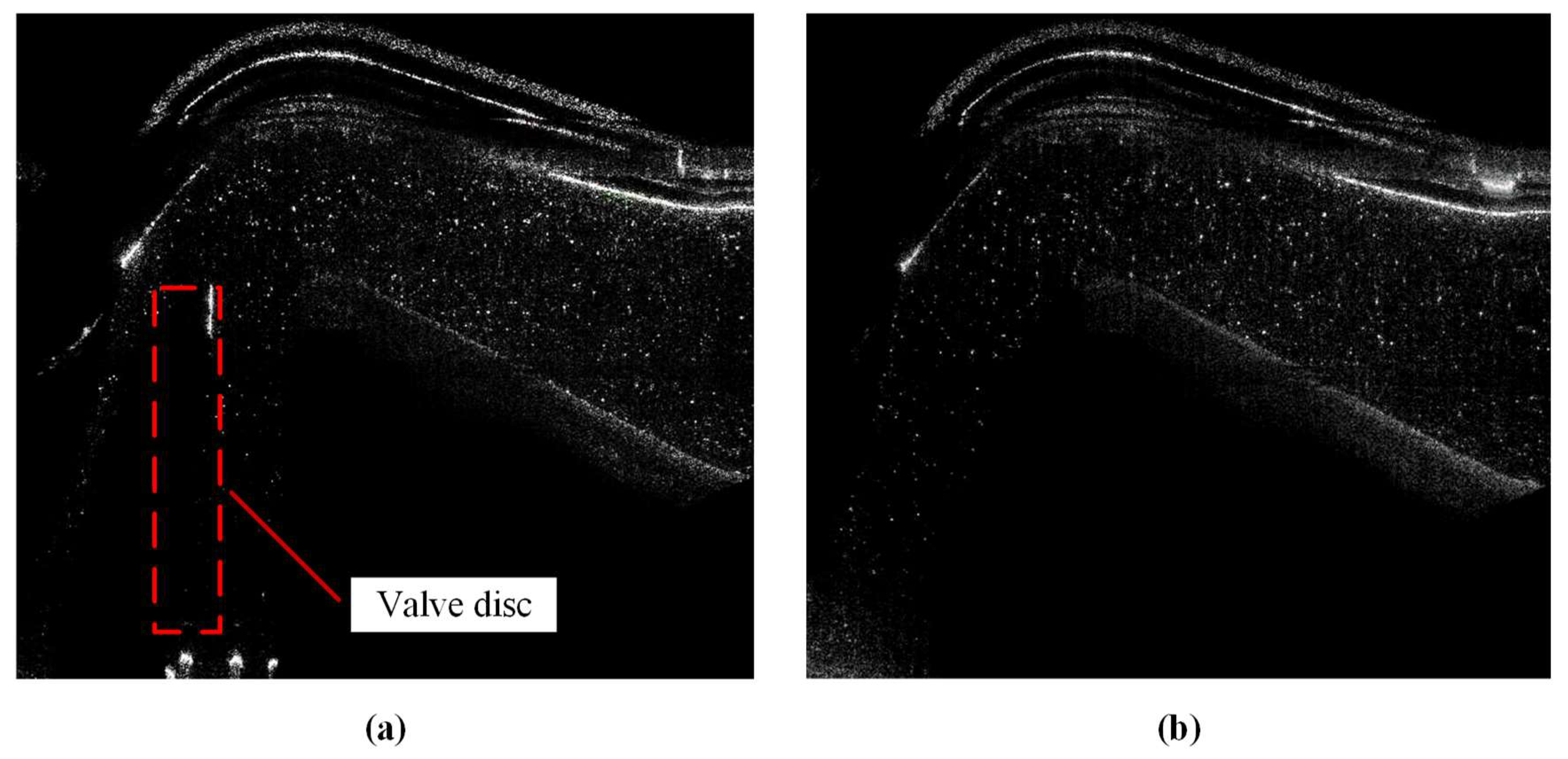
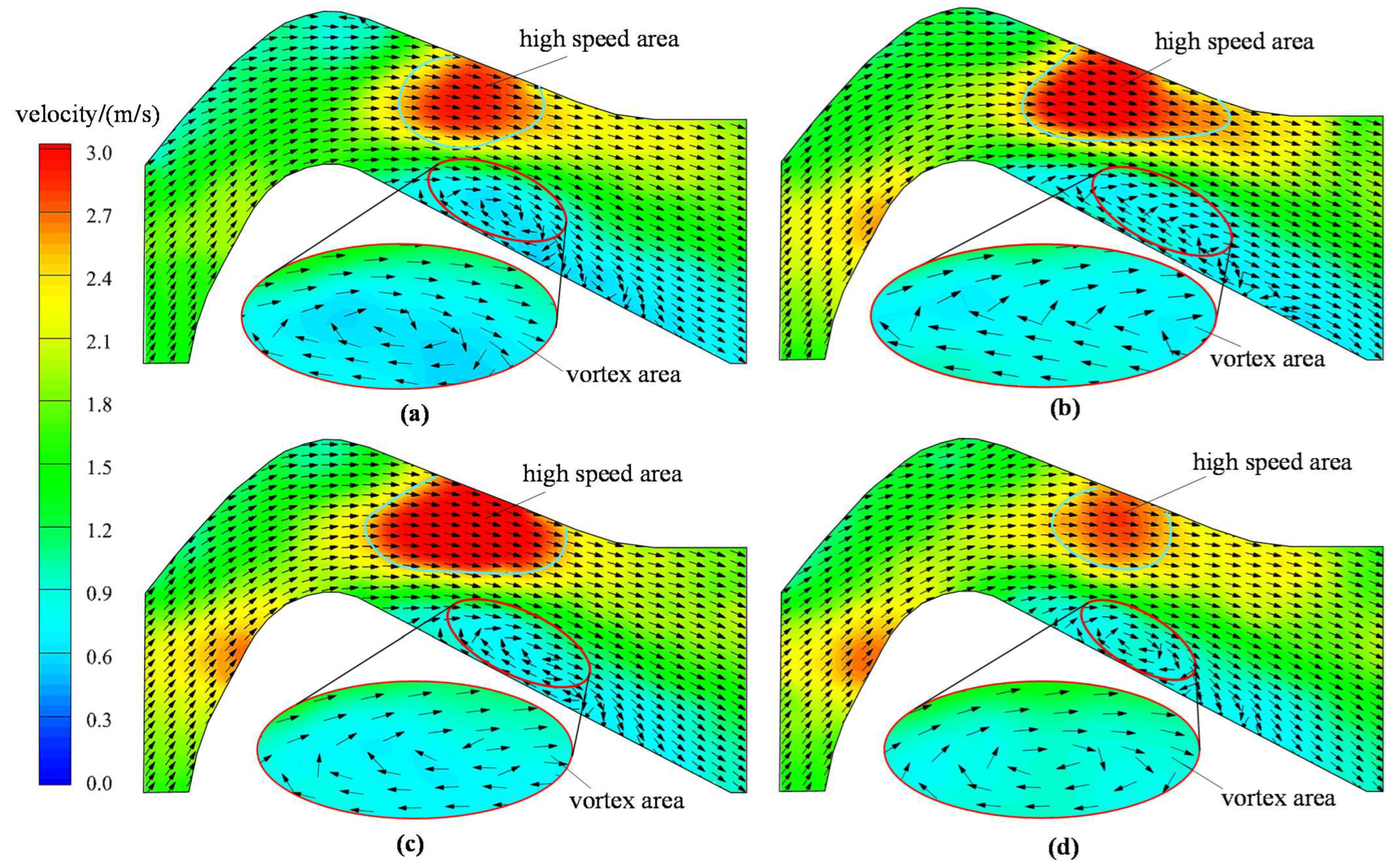
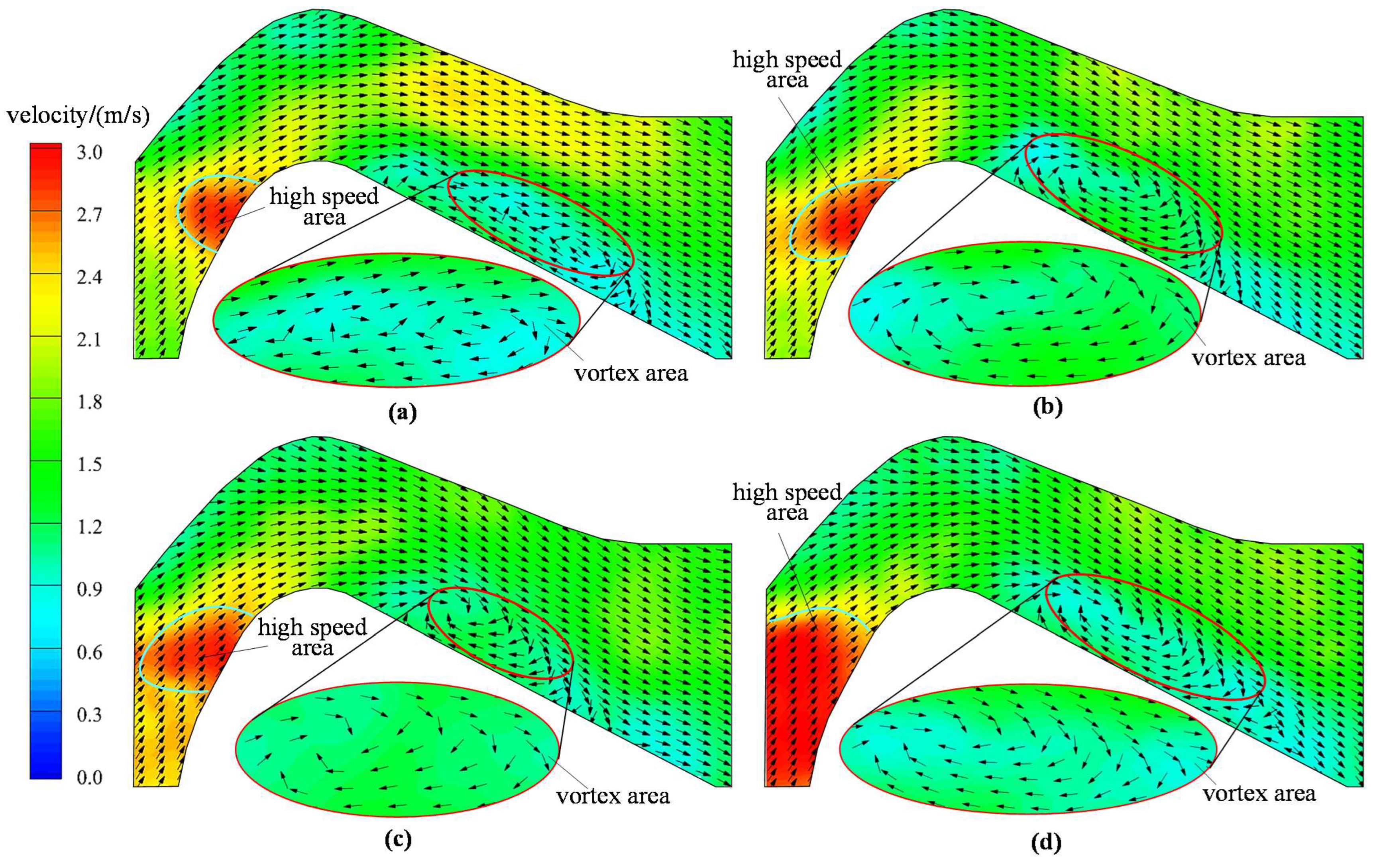
3.1.2. Flow Field Analysis

Figure 10, Figure 11 and Figure 12 show the nozzle check valve axial plane flow field at the low flow rate, medium flow rate, and high flow rate, respectively. Under a low flow rate, as in Figure 10a, the valve disc displacement is small, and the main flow carries the vortex flow formed in the gap between the valve disc and the downstream deflector to the descending section. The flow passage of the descending segment creates a high-speed zone near the valve body and a vortex zone near the downstream deflector. The flow velocity increases along normal to the flow passage of the descending section, forming a large velocity gradient, and the flow becomes turbulent. What can explain this phenomenon is as follows. When the flow rate is low, the upstream incoming velocity is small, and the fluid bypassing the disc forms a thicker fluid boundary layer at the downstream deflector. The boundary layer flow has a high rotation and normal velocity gradient, resulting in a lower pressure in the boundary layer. The high-speed fluid in the potential flow area flows downstream, causing the downstream pressure to increase, forming a reverse pressure gradient in the boundary layer along the flow direction, which results in the fluid back-flowing and the boundary layer separating.

The disc reaches a large displacement, as shown in Figure 10b, and the vortex flow restrained by the narrower gap is difficult to be carried by the main flow to the descending section. When the main flow bypassing the downstream deflector flows through the curved flow passage of the descending segment, due to fluid inertia, the squeezed fluid near the valve body flows rapidly, forming a local high-speed area. On the other hand, the diffused fluid near the downstream deflector flows slowly, generating a higher normal to velocity gradient, resulting in strongly shear flow and a clockwise vortex area. When the flow rate increases to the point where the valve disc can fully open, as in Figure 10c,d, forming an independent local vortex zone near the downstream deflector causes little disturbance to the downstream flow field, and the flow becomes smoother. The vortex zone migrates toward the top of the downstream deflector as the flow increases. The local high-speed area near the valve body expands with the rise of flow, and in this area, the maximum flow velocity can reach 2 m/s. It is possible to explain this phenomenon by the following points. The flow passage becomes smooth due to fully opening the disc, and fluid forms a morphologically stable boundary layer attached to the downstream deflector wall. At a low flow rate, the thicker boundary layer has wrapped the vortex region, which hardly disturbs the downstream flow field, and the flow velocity in the local high-speed area increases with the flow rate rise. As the flow rate increases, the inverse pressure gradient in the boundary layer enhances, resulting in the migration of the vortex region to the top of the downstream deflector.

In addition, in Figure 10c,d, when the valve disc is fully open, creating the flexing flow passage of the ascending segment, the fluid is squeezed due to flow inertia, resulting in a local high-speed zone near the valve disc, which expands with the flowrate increases.

In the medium flow rate (see Figure 11), the flow velocity of the high-speed area in the flow passage of the descending segment can reach 3 m/s and decreases continuously as the flow rate increases, which is because the boundary layer becomes thinner at a higher flow rate. The vortex escaping from the thinner boundary layer spreads to the mainstream area, resulting in the expansion of the vortex area, which consumes the kinetic energy of the mainstream. As the flow rate increases, the increasing strength vortex consumes more kinetic energy from the mainstream, causing a decrease in the flow velocity of the high-speed area in the descending segment and the flow velocity gradient along the normal to the flow passage gradually. In addition, the local high-speed zone in the ascending section near the valve disc continues to increase and extend to the valve inlet.

When the flow rate reaches a high flow rate (see Figure 12), as the flow rate increases, the local high-speed area in the descending section gradually disappears, reducing the flow velocity gradient along the normal to the flow passage. The reason is that the continuously expanding vortex area spreads to the mainstream, occurring the fluid mass points mix and its momentum exchanges, resulting in the flow velocity tending to be uniform. Besides, as the flow rate increases, the local high-speed zone near the disc continuously expands to the valve inlet, where maximum flow velocity can reach 3 m/s, enhancing the fluid velocity gradient along the flow direction in the ascending segment.

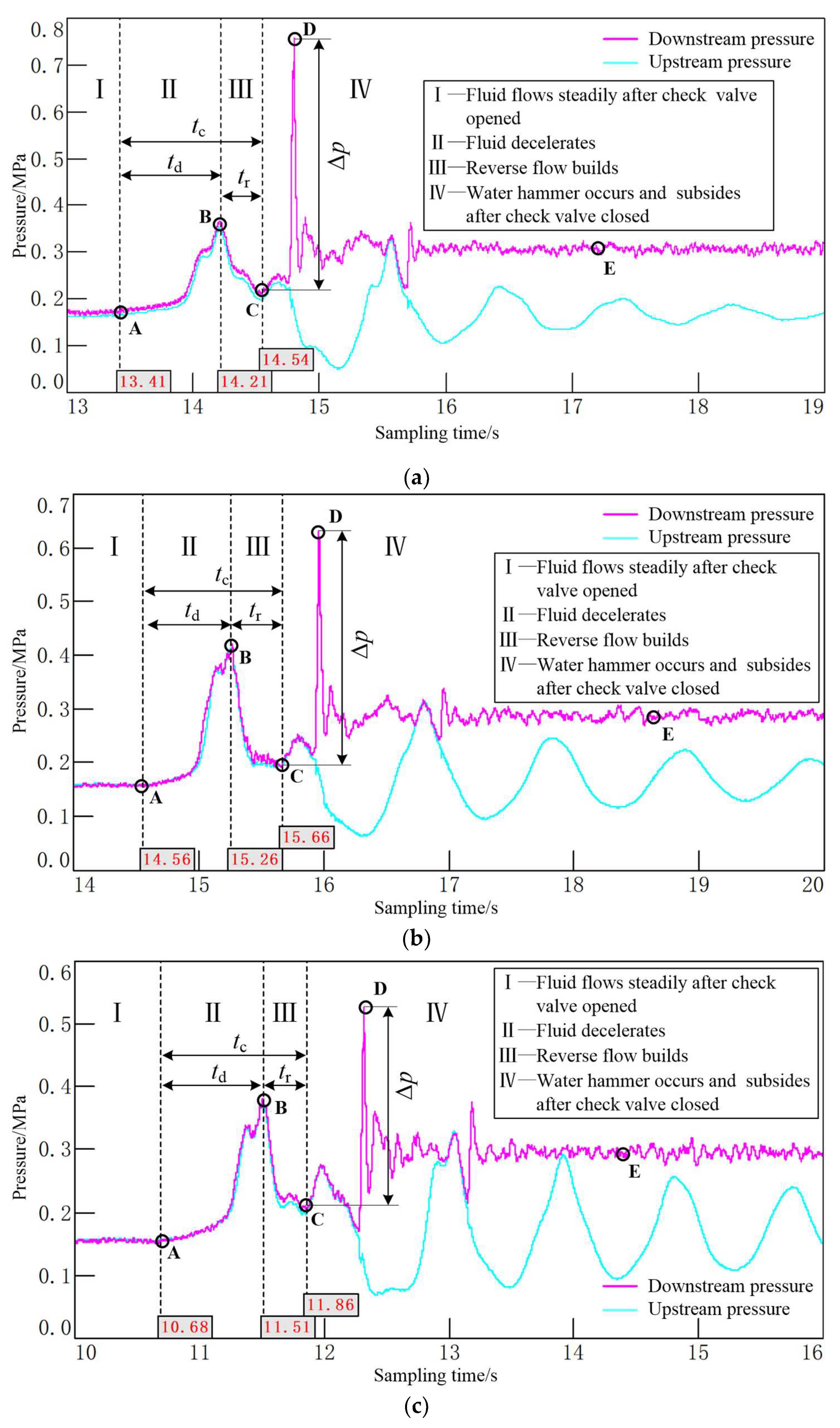
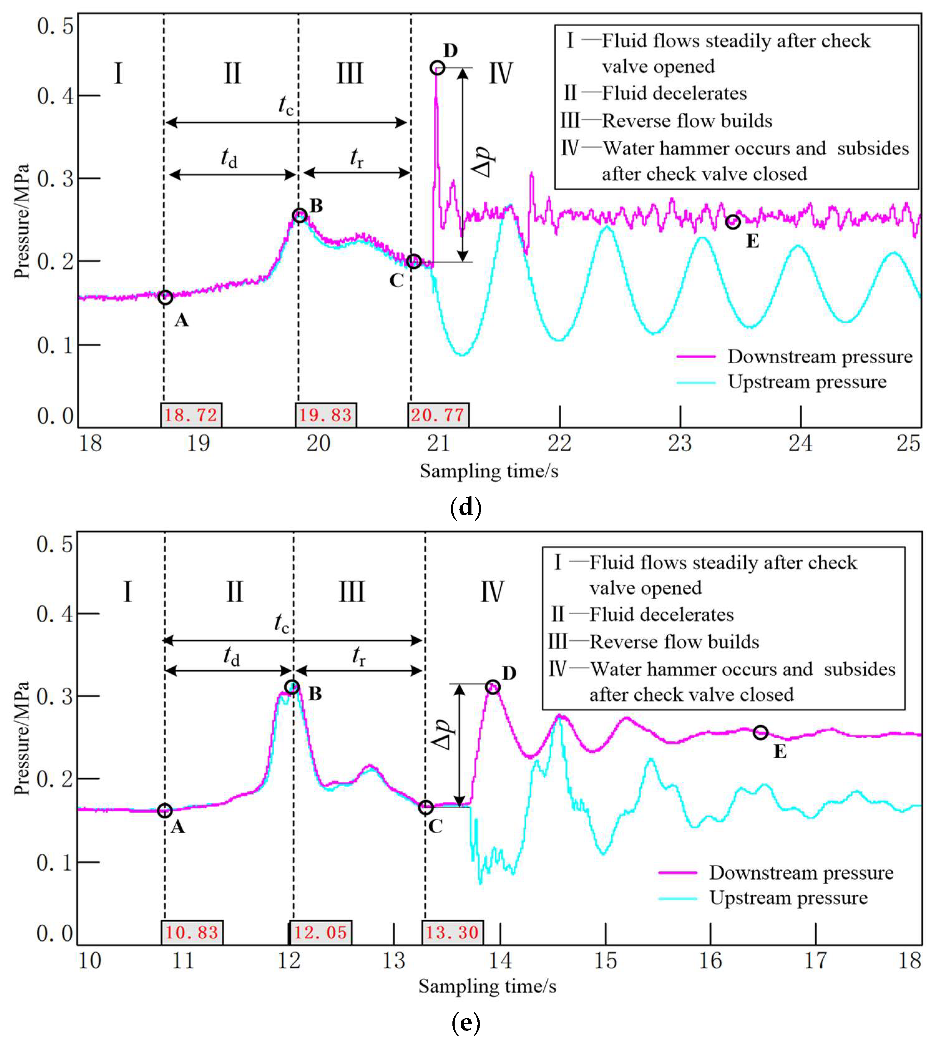
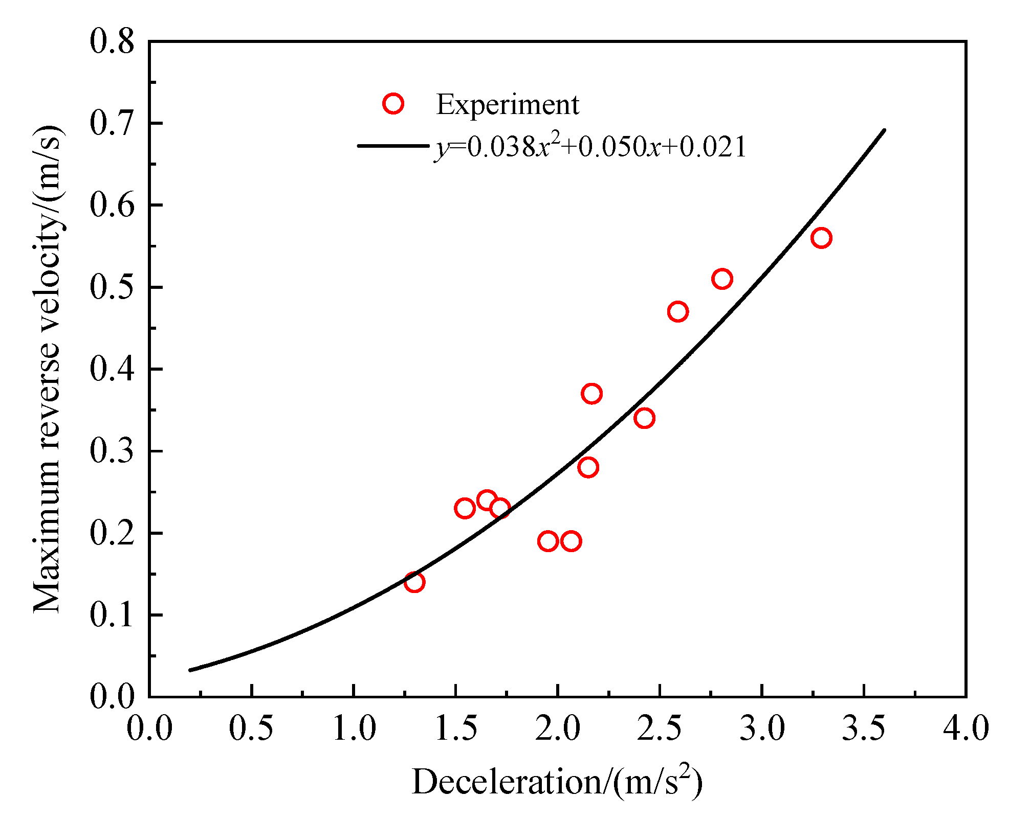
3.2. Nozzle Check Valve Dynamic Behavior Analysis

Figure 13 shows the change of upstream and downstream pressure of the check valve with time for different fluid decelerations in the experimental system, including four stages. (I) The valve is open, the difference between upstream and downstream pressure is little and remains constant, and the fluid flows steadily. The valve disc is affected to spring force, support force, and fluid pressure, which balance each other. (II) The suddenly increasing downstream pressure disrupts the original balancing state, resulting in the disc beginning to close (point A). The growing rising downstream pressure is transferred to the upstream, resulting in a simultaneous increase in upstream and downstream pressures, and the fluid column decelerates. Flow stops when upstream and downstream pressures are almost equal (point B). (III) The disc closes acceleratively with the spring stretching continuously, and the pushed by the disc liquid column backflows. The pressure energy of the fluid transforms into its kinetic energy, resulting in the upstream and downstream pressure decreasing simultaneously with the reverse flow. The check valve finally closes with the valve slamming when reverse flow accelerates to the maximum velocity (point C) [31]. (IV) The kinetic energy instantly converts into pressure energy with the valve slamming, generating the higher water hammer downstream (point D). The water hammer pressure energy dissipates by pipe friction, vibration, and noise, and the downstream pressure recovers to the centrifugal pump outlet pressure (point E). Meanwhile, subject to the high pool pressure, the upstream pressure is momentarily reduced, which maintains the fluctuations in which the amplitude decreases [32], and it finally reaches the initial state pressure (the pressure of the high pool).

It is easy to find in Figure 13 that the lower the fluid deceleration, the lower the water hammer pressure peak. According to Equation (7), in the case of constant decelerating time t_d, reducing the flow rate of steady flow Q₀ can reduce the fluid deceleration. Furthermore, in the case of the fixed flow rate of stable flow, increasing the decelerating time t_d can also reduce the flow deceleration. Reducing the flow rate causes a decrease in the pressure energy stored downstream during the fluid decelerating stage, and the maximum reverse velocity v_R decreases during the fluid reverse flowing. Similarly, the valve disc closure time grows during the decelerating flow stage, resulting in the disc closing to a smaller opening, which leads to the maximum reverse velocity v_R decreasing due to flow resistance increasing. According to Equation (11), the maximum reverse velocity v_R declines, the lower the water hammer pressurization.

Table 2. The testing data of the nozzle check valve dynamic characteristics.

No.	Q0/(m3/h)	td/s	Δp/MPa	dv/dt/(m/s2)	vR/(m/s)
1	403	1.22	0.14	1.30	0.14
2	464	1.18	0.23	1.55	0.23
3	467	1.11	0.24	1.65	0.24
4	485	1.11	0.23	1.72	0.23
5	472	0.95	0.19	1.95	0.19
6	473	0.90	0.19	2.07	0.19
7	443	0.81	0.28	2.15	0.28
8	496	0.90	0.37	2.17	0.37
9	512	0.83	0.34	2.43	0.34
10	461	0.70	0.47	2.59	0.47
11	571	0.80	0.51	2.81	0.51
12	561	0.67	0.56	3.29	0.56

shows the dynamic characteristics testing data of the nozzle check valve, using these data to plot the dynamic characteristics curve (see Figure 14), the graph reveals that the maximum reverse velocity increases with the boost of fluid deceleration below 4 m/s², whose growing trend satisfies the quadratic curve y = 0.038x² + 0.050x + 0.021. The slope of the curve meets y = 0.076x + 0.050, whose maximum is 0.354, which reflects the response of the nozzle check valve to the system. The smaller the slope of the curve, the better response of the check valve. The ideal curve slope is zero, in which the maximum reverse velocity is constant with the fluid deceleration varying. This ideal check valve can adaptively adjust closing.

The valve designer can design a better performance check valve by reducing the slope of the dynamic characteristic curve by making several measures. In addition, if the valve manufacturer provides a dynamic characteristic curve, the engineers who know the system deceleration can be a convenient and reasonable selection of check valve and pipeline withstanding a certain pressure by using this curve, which considerably saves costs. At the same time, when engineers who know the maximum acceptable pressure of the piping system need to adjust the system working condition, they can safely and effectively regulate the required working condition by using this curve to change the system deceleration. It significantly reduces the risk of piping system bursts caused by improper operation.

4. Conclusions

In the present work, to investigate the hydraulic losses and safe operation of nozzle check valves in industrial piping systems, the static characteristics of the valve and its dynamic behavior in the pipeline system were studied using an experimental bench with a visual DN300 nozzle check valve. Besides, based on the PIV technique measures the valve steady-state flow field under the different flow rates.

In the static experiment, when the flow rate rises to 16 m³/h, the valve disc displacement increases instantaneously from zero to 26 mm; as the flow rate rises, the valve disc displacement slowly increases to 44 mm, then rapidly grows to a maximum displacement of 72 mm. When the valve is not fully open, the upstream and downstream pressure drop improves slowly as the flow rate rises; however, when the Reynolds number exceeds 5 × 10⁵ (valve fully opening), the relationship between pressure drop and flow obeys a quadratic function.

PIV flow field test results show that the local vortex area formed by the flow passage near the downstream deflector expands with the flow improvement. As the increase of flowrate, at low flow work, the downstream flow velocity in the local high-speed area near the valve body increases; at medium flow work, the area’s flow velocity decreases; at high flow work, this local high-speed area disappears.

In the experiment of the dynamic behavior, the check valve closing process includes two stages. In the first, the valve begins to close with the upstream and downstream pressure increasing synchronously, and the liquid column decelerates until the flow stops. In the second, the valve continues closing with the pressure decreasing synchronously, generating reverse flow, which accelerates to the maximum velocity, the valve finally closes, and valve slamming occurs. In the fluid deceleration below 4 m/s², the dynamic characteristics curve meets the secondary function, whose maximum slope is only 0.354, reflecting that the nozzle check valve has a favorable response to the system.

Therefore, firstly, considering the static characteristics of the check valve can provide a reference for selecting the right power working machine (pump or compressor). Secondly, by understanding the flow field characteristics inside the check valve through PIV technology, the designer can change the flow passage structure to avoid vortex flow as much as possible, thus reducing the hydraulic losses. Finally, knowing the dynamic behavior can be convenient in designing and selecting a check valve and regulating piping system working conditions. In further research, it is likely an effective method to study dynamic characteristics that utilize the high-speed PIV technique to measure the flow field characteristics of the check valve closing process.

References

1. Karpenko, M.; Prentkovskis, O.; Šukevičius, Š. Research on high-pressure hose with repairing fitting and influence on energy parameter of the hydraulic drive. Eksploat. Niezawodn.-Maint. Reliab. 2022, 24, 25–32. [Google Scholar] [CrossRef]
2. Urbanowicz, K.; Bergant, A.; Kodura, A.; Kubrak, M.; Malesińska, A.; Bury, P.; Stosiak, M. Modeling transient pipe flow in plastic pipes with modified discrete bubble cavitation model. Energies 2021, 14, 6756. [Google Scholar] [CrossRef]
3. Sibilla, S.; Gallati, M. Hydrodynamic characterization of a nozzle check valve by numerical simulation. J. Fluids Eng. 2008, 130, 121101. [Google Scholar] [CrossRef]
4. Botros, K.K.; Richards, D.J.; Roorda, O. Effect of check valve dynamics on the sizing of recycle systems for centrifugal compressors. In Proceedings of the ASME 1996 International Gas Turbine and Aeroengine Congress and Exhibition, Birmingham, UK, 10 June 1996; American Society of Mechanical Engineers: New York, NY, USA, 1996. [Google Scholar]
5. Lai, Z.; Li, Q.; Karney, B.; Yang, S.; Wu, D.; Zhang, F. Numerical Simulation of a Check Valve Closure Induced by Pump Shutdown. J. Hydraul. Eng. 2018, 144, 06018013. [Google Scholar] [CrossRef]
6. Li, G.; Liou, J.C.P. Swing check valve characterization and modeling during transients. In Proceedings of the ASME/JSME 2003 4th Joint Fluids Summer Engineering Conference, Honolulu, HI, USA, 6–10 July 2003; Volume 1: Fora, Parts A, B, C, and D, pp. 2839–2846. [Google Scholar]
7. Guivier-Curien, C.; Deplano, V.; Bertrand, E. Validation of a numerical 3-D fluid–structure interaction model for a prosthetic valve based on experimental PIV measurements. Med. Eng. Phys. 2009, 31, 986–993. [Google Scholar] [CrossRef] [PubMed]
8. Corvaro, F.; Marchetti, B.; Vitali, M. Validation of velocity field measured with particle image velocimetry of a partially heated cavity. Heat Transf. Eng. 2022, 1–3. [Google Scholar] [CrossRef]
9. Capanna, R.; Bardet, P.M. High speed PIV measurements in water hammer. In Proceedings of the 14th International Symposium on Particle Image Velocimetry, Online, 1–4 August 2021. [Google Scholar]
10. Dobrev, I.; Massouh, F. CFD and PIV investigation of unsteady flow through Savonius wind turbine. Energy Procedia 2011, 6, 711–720. [Google Scholar] [CrossRef] [Green Version]
11. Shen, L.; Willman, C.; Stone, R.; Lockyer, T.; Magnanon, R.; Virelli, G. On the use of particle image velocimetry (PIV) data for the validation of Reynolds averaged Navier-Stokes (RANS) simulations during the intake process of a spark ignition direct injection (SIDI) engine. Int. J. Engine Res. 2022, 23, 1061–1081. [Google Scholar] [CrossRef]
12. Provoost, G.A. The Dynamic Behavior of Non-Return Valves. In Proceedings of the Third International Conference on Pressure Surges, Canterbury, UK, 25–27 March 1980. [Google Scholar]
13. Thorley, A.R.D. Check Valve Behavior Under Transient Flow Conditions: A State-of-the-Art Review. J. Fluids Eng 1989, 111, 178–183. [Google Scholar] [CrossRef]
14. Botros, K.K. Spring stiffness selection criteria for nozzle check valves employed in compressor stations. J. Eng. Gas Turbines Power 2011, 133, 122401. [Google Scholar] [CrossRef]
15. Rao, P.V.; Achar, K.R.T.; Rao, P.L.N.; Purcell, P.J. Case study of check-valve slam in rising main protected by air vessel. J. Hydraul. Eng. 1999, 125, 1166–1168. [Google Scholar] [CrossRef]
16. Yang, Z.; Zhou, L.; Dou, H.; Lu, C.; Luan, X. Water hammer analysis when switching of parallel pumps based on contra-motion check valve. Ann. Nucl. Energy 2020, 139, 107275. [Google Scholar] [CrossRef]
17. Kim, N.S.; Jeong, Y.H. An investigation of pressure build-up effects due to check valve’s closing characteristics using dynamic mesh techniques of CFD. Ann. Nucl. Energy 2020, 152, 107996. [Google Scholar] [CrossRef]
18. Wang, H.M.; Chen, S.; Li, K.L.; Li, H.Q.; Yang, Z. Numerical study on the closing characteristics of a check valve with built-in damping system. J. Appl. Fluid Mech. 2021, 14, 1003–1014. [Google Scholar]
19. Mk, A.; Ak, B.; Es, B. Analytical and CFD analysis investigation of fluid-structure interaction during water hammer for straight pipe line. Int. J. Press. Vessel. Pip. 2021, 194, 104528. [Google Scholar]
20. Lai, Z.; Karney, B.; Yang, S.; Wu, D.; Zhang, F. Transient performance of a dual disc check valve during the opening period. Ann. Nucl. Energy 2017, 101, 15–22. [Google Scholar] [CrossRef]
21. Himr, D.; Habán, V.; Hudec, M.; Pavlík, V. Experimental investigation of the check valve behaviour when the flow is reversing. EPJ Web Conf. 2017, 143, 02036. [Google Scholar] [CrossRef] [Green Version]
22. Himr, D.; Habán, V.; Hudec, M. Experimental investigation of check valve behaviour during the pump trip. J. Phys. Conf. Ser. 2017, 813, 012054. [Google Scholar] [CrossRef] [Green Version]
23. Himr, D.; Habán, V.; Závorka, D. Axial check valve behaviour during flow reversal. IOP Conf. Ser. Earth Environ. Sci. 2019, 405, 012012. [Google Scholar] [CrossRef]
24. Westerweel, J. Fundamentals of digital particle image velocimetry. Meas. Sci. Technol. 1997, 8, 1379. [Google Scholar] [CrossRef] [Green Version]
25. Clément, S.A.; André, M.A.; Bardet, P.M. Multi-spatio-temporal scales PIV in a turbulent buoyant jet discharging in a linearly stratified environment. Exp. Therm. Fluid Sci. 2021, 129, 110429. [Google Scholar] [CrossRef]
26. Pérez, J.M.; Sastre, F.; Le Clainche, S.; Vega, J.M.; Velazquez, A. Three-dimensional flow field reconstruction in the wake of a confined square cylinder using planar PIV data. Exp. Therm. Fluid Sci. 2022, 133, 110523. [Google Scholar] [CrossRef]
27. Gu, M.; Li, J.; Xu, C. A modified Richardson–Lucy deconvolution for rapid reconstruction of light field μPIV. Exp. Fluids 2022, 63, 1–15. [Google Scholar] [CrossRef]
28. Pastrana, H.; Treviño, C.; Pérez-Flores, F.; Martínez-Suástegui, L. TR-PIV measurements of turbulent confined impinging twin-jets in crossflow. Exp. Therm. Fluid Sci. 2022, 136, 110667. [Google Scholar] [CrossRef]
29. Joukowsky, N. Über den Hydraulischen Stoss in Wasserleitungsrohren; Series 8; Mémoires de l’Académie Impériale des Sciences: St.-Pétersbourg, Russia, 1900. [Google Scholar]
30. Thorley, A.R.D. Fluid Transients in Pipeline Systems; D&L George Ltd.: Herts, UK, 1991. [Google Scholar]
31. Ballun, J.V. A methodology for predicting check valve slam. Am. Water Work. Assoc. 2007, 99, 60–65. [Google Scholar] [CrossRef]
32. Sra, B.; Ar, A. Experimental investigation of viscoelastic turbulent fluid hammer in helical tubes, considering column-separation. Int. J. Press. Vessel. Pip. 2021, 194, 104489. [Google Scholar]
Figure 1. Structure diagram of the nozzle check valve.
Energies 15 05393 g001
Figure 2. PIV flow velocity measurement system.
Energies 15 05393 g002
Figure 3. Nozzle check valve test system.
Energies 15 05393 g003
Figure 4. Flow chart of static characteristics test of nozzle check valve.
Energies 15 05393 g004
Figure 5. Flow chart of dynamic behavior test of nozzle check valve.
Energies 15 05393 g005
Figure 6. Physical diagram of the test system in the field. (a) Pipeline system; (b) LMS data acquisition system; (c) Particle image velocimetry system.
Energies 15 05393 g006
Figure 7. Images of a flow passage with tracer particles taken by a CCD camera. (a) Partially opened valve; (b) Fully opened valve.
Energies 15 05393 g007
Figure 8. The change curve of valve disc displacement and pressure drop as a function of flow rate. (Note: The displacement of the valve disc is zero in the fully closed position and is a positive value with the direction of the opening disc).
Energies 15 05393 g008
Figure 9. The dimensionless hydraulic loss curve of the nozzle check valve.
Energies 15 05393 g009
Figure 10. Flow field characteristics at low flow rates. (a) Q = 76 m3/h; (b) Q = 173 m3/h; (c) Q = 305 m3/h; (d) Q = 356 m3/h.
Energies 15 05393 g010
Figure 11. Flow field characteristics at medium flow rates. (a) Q = 407 m3/h; (b) Q = 458 m3/h; (c) Q = 509 m3/h; (d) Q = 560 m3/h.
Energies 15 05393 g011
Figure 12. Flow field characteristics at high flow rates. (a) Q = 610 m3/h; (b) Q = 661 m3/h; (c) Q = 712 m3/h; (d) Q = 763 m3/h.
Energies 15 05393 g012
Figure 13. Transient pressure testing curves at different decelerations. (a) dv/dt = 2.81 m/s2; (b) dv/dt = 2.59 m/s2; (c) dv/dt = 2.43 m/s2; (d) dv/dt = 1.72 m/s2; (e) dv/dt = 1.29 m/s2.
Energies 15 05393 g013aEnergies 15 05393 g013b
Figure 14. The testing data of the nozzle check valve dynamic characteristics.
Energies 15 05393 g014