Investigation of Energy-Saving Strategy for Parallel Variable Frequency Pump System Based on Improved Differential Evolution Algorithm

Abstract

This paper presents an energy-saving strategy that was applied to a parallel variable frequency pump system of a water circulation pumping station. Firstly, the mathematical model of shaft power consumption for the parallel pump system was established using quadratic polynomial fitting, with some constraints configured according to the system’s water supply demands. Then, the algorithm program was designed with the goal of minimizing the energy consumption through the application of an improved differential evolution algorithm. Additionally, the energy consumption model and constraints were integrated and simplified in order to adapt to the algorithm calculation. In the end, the algorithm was implemented according to the pump design parameters and supply targets of the pumping station. Meanwhile, a comparison was done between the differential evolution (DE) algorithm and the genetic algorithm (GA). Furthermore, an experimental test was conducted in an aluminum company in order to verify the applicability of the energy-saving algorithm in practice. The results demonstrated the feasibility of using the improved differential evolution algorithm in order to achieve a minimum energy consumption operation strategy; the results consequently manifested the superiority of the differential evolution algorithm in both computing time and optimal solution aspects.

1. Introduction

Energy is a fundamental part of civil life and industrial development. As a result of the rapidly developing modern economy and the surging global population, an energy shortage problem is becoming increasingly apparent [1]. Energy consumption is estimated to increase by at least 30% from 2016 to 2030. Energy conservation has become a prominent issue all over the world [2]. Accordingly, reducing energy consumption and improving energy utilization are becoming increasingly crucial to energy enterprises.

According to statistics, the energy consumption of overall pump systems accounts for more than 20% of total global industrial energy consumption [3]. Nevertheless, the actual efficiencies of many pump operations are very low, especially in some developing countries. Therefore, the pump system has considerable energy-saving potential from the perspective of system optimization during operation. In summary, pump energy saving is a system-wide project that is infeasible to realize only through improving the efficiency of pump products.

In order to improve the operation efficiency of a parallel pump unit, it is essential to monitor and collect information regarding its operation state in real time. The data of its working condition can then be analyzed in order to design and implement energy saving schemes.

Methods for solving the energy-saving problem can be found in the literature. Based on the statistical analysis of energy consumption data, Yang [4] conducted a retrofit test on a certain oil transmission pump, and summarized the advantages of using an energy monitoring system to guide the operation strategy of the pump equipment. By comparing the economic benefits and establishing the energy prediction model, the energy consumption monitoring system was further upgraded, which helped managers comprehensively determine the best technical scheme. Muljadi et al. [5] proposed an optimization framework based on a dynamic programming algorithm, which was used for optimizing the energy efficiency of a parallel pump system controlled by a PLC. Xu [6] added a frequency converter to the motor of a circulating pump system. It achieved improvements in energy savings, emissions reduction and automated management, which reduced both energy consumption and labor costs for enterprises. Meanwhile, the frequency conversion transformation-realized soft start method played a critical role in the operation and maintenance of the system. With developments in computer technology and improvements in computing power, the use of artificial intelligence optimization algorithms is more frequently being explored and applied. On this basis, a series of calculation methods catering to different scheduling models have been established, such as the genetic algorithm, simulated annealing algorithm, particle swarm optimization algorithm and artificial neural network algorithm [7,8]. De Wrachien et al. [9] developed and improved the genetic algorithm (GA) for the optimization of pump operations in water distribution networks in terms of both energy and economic savings. Significant progress has been made in the transition from a discrete to a continuous description of pump operation. Lai [10] established an optimization model for a parallel pump unit. The actual working point was limited in achieving an optimal efficiency point of the centrifugal pumps due to constraints; particle swarm optimization algorithm was introduced to solve the problem, which resulted in efficient and reliable operation of the centrifugal pumps. Baranidharan et al. [11] proposed an adaptive neuro-fuzzy inference system (ANFIS) to decrease overall losses and enhance energy savings in pump systems. It is a deep learning method that combines adaptive control, artificial neural networks and fuzzy inference systems. Abdelsalam et al. [12] utilized an artificial electric field algorithm (AEFA) to control the on/off operation of water pumps, in order to minimize the costs of energy consumption as well as the number of pumps switching in water networks. It is an iterative process that includes an optimization algorithm and the EPANET hydraulic simulator. Its findings revealed that AEFA is superior in terms of convergence and cost savings in energy consumption. The differential evolution algorithm, which gained attention in research later, had better comprehensive performance in terms of convergence, optimization ability and robustness [13]. Accordingly, there is currently particular research value in using the differential evolution algorithm to solve optimization problems in pump operations.

This paper focuses on the parallel variable frequency pump unit as its research objective, with emphasis on achieving energy saving and consumption reduction for this type of pump system. A method that uses improved differential evolution algorithm is proposed and applied in this study, in order to offer an optimal frequency conversion control scheme according to different water supply requirements. The parallel variable frequency pump unit can reduce the overall energy consumption of the system by the greatest extent on the premise of meeting the system’s performance demands.

This paper is arranged as follows: in Section 2, the energy consumption model and constraints of the parallel variable frequency pump system are established using quadratic polynomial fitting; in Section 3, the improved differential evolution algorithm is introduced and utilized to solve this optimal scheduling model; in Section 4, the program is designed and implemented by using Python IDE, according to the simplified fitness function model. The results of the optimal solution and iteration process of algorithm are illustrated. Moreover, the results of the differential evolution algorithm and genetic algorithm are compared. In Section 5, an experimental test is conducted in order to verify the applicability as well as the economic performance of the algorithm in a practical scenario. In Section 6, conclusions are drawn about the optimal scheduling method for a parallel variable frequency pump system, and the prospects of follow-up research are put forward.

2. Establishment of Energy Consumption Model of Parallel Pump System

With developments in industrial production technology, concentration on energy-saving transformations has shifted away from optimizing single equipment to optimizing systems overall. The main research content of this subject can be divided into two aspects related to energy saving for a parallel variable frequency pump system (PVFPS), as shown in Figure 1. One aspect is the pump energy consumption model of the PVFPS, while the other aspect is the optimal control scheme of the PVFPS, namely the solver of the scheduling model.

Figure 1 is a simplified schematic diagram of the PVFPS. VFD is the variable frequency drive, and the numbers of the parallel constant speed pumps and speed regulating pumps in this system are three and two, respectively.

By means of the frequency conversion regulation of the pump in parallel operation, the characteristic curve and working point of the pump can be modified, in order to meet the flow and head of different control requirements. A reasonable frequency conversion control strategy plays a vital role in energy saving and consumption reduction of a PVFPS.

In this section, the water supply target (Q_t, H_t) will be taken as the basic control index, and the total energy consumption (shaft power J) of the pump system will be calculated as the optimization goal. Assuming that the parallel pump unit configuration of the water supply system is composed of M constant speed pumps and N speed regulating pumps, the goal function of this optimization problem can be expressed as follows:

$${\mathrm{J}=\mathrm{n}}_1\left({\mathrm{b}}_{10 }{+\mathrm{b}}_{11}{\mathrm{Q}}_1{+\mathrm{b}}_{12}{\mathrm{Q}}_1^{ 2}{+\mathrm{b}}_{13}{\mathrm{Q}}_1^{ 3}\right){+\mathrm{n}}_2\left({\mathrm{b}}_{20}{\mathrm{s}}^{ 3}{+\mathrm{b}}_{21}{\mathrm{s}}^{ 2}{\mathrm{Q}}_2{+\mathrm{b}}_{22}{\mathrm{sQ}}_2^{ 2}{+\mathrm{b}}_{23}{\mathrm{Q}}_2^{ 3}\right)$$

(1)

where J is the sum of shaft power of pump unit; n₁ $\in$ [0, M] and n₂ $\in$ [0, N] are the numbers of constant speed and speed regulating pumps put into parallel operation separately, respectively; Q₁, Q₂ and s are the working flow and the speed regulation ratio of pump, respectively; b_i0, b_i1, b_i2 and b_i3 (I = 1, 2) are the fitting coefficients of P-Q characteristic curve of each pump by the theory of the least square polynomial.

Most importantly, there are several constraints that should be taken into account before solving the mathematical model of this optimization problem. In order to satisfy the water supply target (Q_t, H_t), we define the following:

$$\left\{\begin{array}{c}{ \mathrm{Q}}_{\mathrm{t}} \le { \mathrm{n}}_1{\mathrm{Q}}_1{+\mathrm{n}}_2{\mathrm{Q}}_2\\ {\mathrm{H}}_{\mathrm{t}}{=\mathrm{H}}_{1 }{=\mathrm{H}}_2\end{array}\right.$$

(2)

where H₁ and H₂ are the head of the constant speed pumps and the head of the speed regulating pumps, respectively.

Literature [14] found that the efficiency of the pump and motor would be significantly reduced when the rotation speed is less than half of the rated speed, and that more power would be consumed. Therefore, in practical application, the minimum speed regulation ratio of the centrifugal pump is usually more than 0.5. Due to the limitations of support, heat dissipation and lubrication, the working speed of the centrifugal pump and motor is usually lower than the rated speed. Thus, another rule that should be satisfied is defined as follows:

$$0.5 \le \mathrm{s} \le 1$$

(3)

Theoretically, the H-Q characteristic curve of the centrifugal pump under variable frequency operation can be expressed as follows [15]:

$${\mathrm{H}=\mathrm{s} }^2{\mathrm{H}}_{\mathrm{x}}-{\mathrm{S}}_{\mathrm{x}}{\mathrm{Q} }^2$$

(4)

where H and Q are the operating head and flow, respectively; H_x is the virtual head coefficient; and S_x is the virtual impedance coefficient.

Accordingly, Q₁ and Q₂ can be defined as follows:

$${\mathrm{Q}}_1=\sqrt{\frac{{\mathrm{H}}_{\mathrm{x}1 }-{\mathrm{H}}_1}{{\mathrm{S}}_{\mathrm{x}1}}}$$

(5)

$${\mathrm{Q}}_2=\sqrt{\frac{{\mathrm{s}}^2{\mathrm{H}}_{\mathrm{x}2}-{ \mathrm{H}}_2}{{\mathrm{S}}_{\mathrm{x}2}}}$$

(6)

where s should meet the conditions shown as follows:

$$\sqrt{\frac{{\mathrm{H}}_2}{{\mathrm{H}}_{\mathrm{x}2}}} < \mathrm{s} < 1$$

(7)

3. Minimum Energy Consumption Control Strategy

Based on the analysis in Section 2, it can be concluded that the optimization objective of the system is the shaft power of the PVFPS. The optimization problem is transformed into finding the optimal solution of three variables, n₁, n₂ and s, on the premise of meeting the constraint in Equation (2) and the value range of each variable, in order to minimize optimization objective J. After integrating the energy consumption model and its constraints, the simplified problem model based on the differential evolution (DE) algorithm can be obtained, as shown in Equation (8):

$$\begin{array}{c}\mathrm{minJ} = \min \left\{\begin{array}{c}{\mathrm{n}}_1\left({\mathrm{b}}_{10}{+\mathrm{b}}_{11}\sqrt{\frac{{\mathrm{H}}_{\mathrm{x}1}-{ \mathrm{H}}_{\mathrm{t}}}{{\mathrm{S}}_{\mathrm{x}1}}}{+\mathrm{b}}_{12}\frac{{\mathrm{H}}_{\mathrm{x}1}-{ \mathrm{H}}_{\mathrm{t}}}{{\mathrm{S}}_{\mathrm{x}1}}{+\mathrm{b}}_{13}\frac{{\mathrm{H}}_{\mathrm{x}1}-{ \mathrm{H}}_{\mathrm{t}}}{{\mathrm{S}}_{\mathrm{x}1}}\sqrt{\frac{{\mathrm{H}}_{\mathrm{x}1 }-{ \mathrm{H}}_{\mathrm{t}}}{{\mathrm{S}}_{\mathrm{x}1}}}\right)+\\ {\mathrm{n}}_2\left({\mathrm{b}}_{20}{\mathrm{s}}^3{+\mathrm{b}}_{21}{\mathrm{s}}^2\sqrt{\frac{{\mathrm{s}}^2{\mathrm{H}}_{\mathrm{x}2}-{ \mathrm{H}}_{\mathrm{t}}}{{\mathrm{S}}_{\mathrm{x}2}}}{+\mathrm{b}}_{22}\frac{{\mathrm{s}}^3{\mathrm{H}}_{\mathrm{x}2}-{ \mathrm{sH}}_{\mathrm{t}}}{{\mathrm{S}}_{\mathrm{x}2}}{+\mathrm{b}}_{23}\frac{{\mathrm{s}}^2{\mathrm{H}}_{\mathrm{x}2 }-{ \mathrm{H}}_{\mathrm{t}}}{{\mathrm{S}}_{\mathrm{x}2}}\sqrt{\frac{{\mathrm{s}}^2{\mathrm{H}}_{\mathrm{x}2 }-{ \mathrm{H}}_{\mathrm{t}}}{{\mathrm{S}}_{\mathrm{x}2}}}\right)\end{array}\right\}\\ \mathrm{s}.\mathrm{t}{. \mathrm{Q}}_{\mathrm{t}} \le { \mathrm{n}}_1\sqrt{\frac{{\mathrm{H}}_{\mathrm{x}1 }-{ \mathrm{H}}_{\mathrm{t}}}{{\mathrm{S}}_{\mathrm{x}1}}}{+\mathrm{n}}_2\sqrt{\frac{{\mathrm{s}}^2{\mathrm{H}}_{\mathrm{x}2}-{ \mathrm{H}}_{\mathrm{t}}}{{\mathrm{S}}_{\mathrm{x}2}}}\\ 0 \le { \mathrm{n}}_{1 }\le \mathrm{M}, 0 \le { \mathrm{n}}_2 \le \mathrm{N}\\ \hspace{1em}\hspace{1em}\hspace{1em} \sqrt{\frac{{\mathrm{H}}_{\mathrm{t}}}{{\mathrm{H}}_{\mathrm{x}2}}} < \mathrm{s} < 1, 0.5 \le \mathrm{s} \le 1\end{array}$$

(8)

where ${\mathrm{n}}_1$, ${\mathrm{n}}_2$ and $\mathrm{s}$ are three important variables to be solved, while other parameters are constants whose values depend on the pump design parameters and water supply targets. In short, the values of ${\mathrm{n}}_1$, ${\mathrm{n}}_2$ and $\mathrm{s}$ determine the amount of energy consumed.

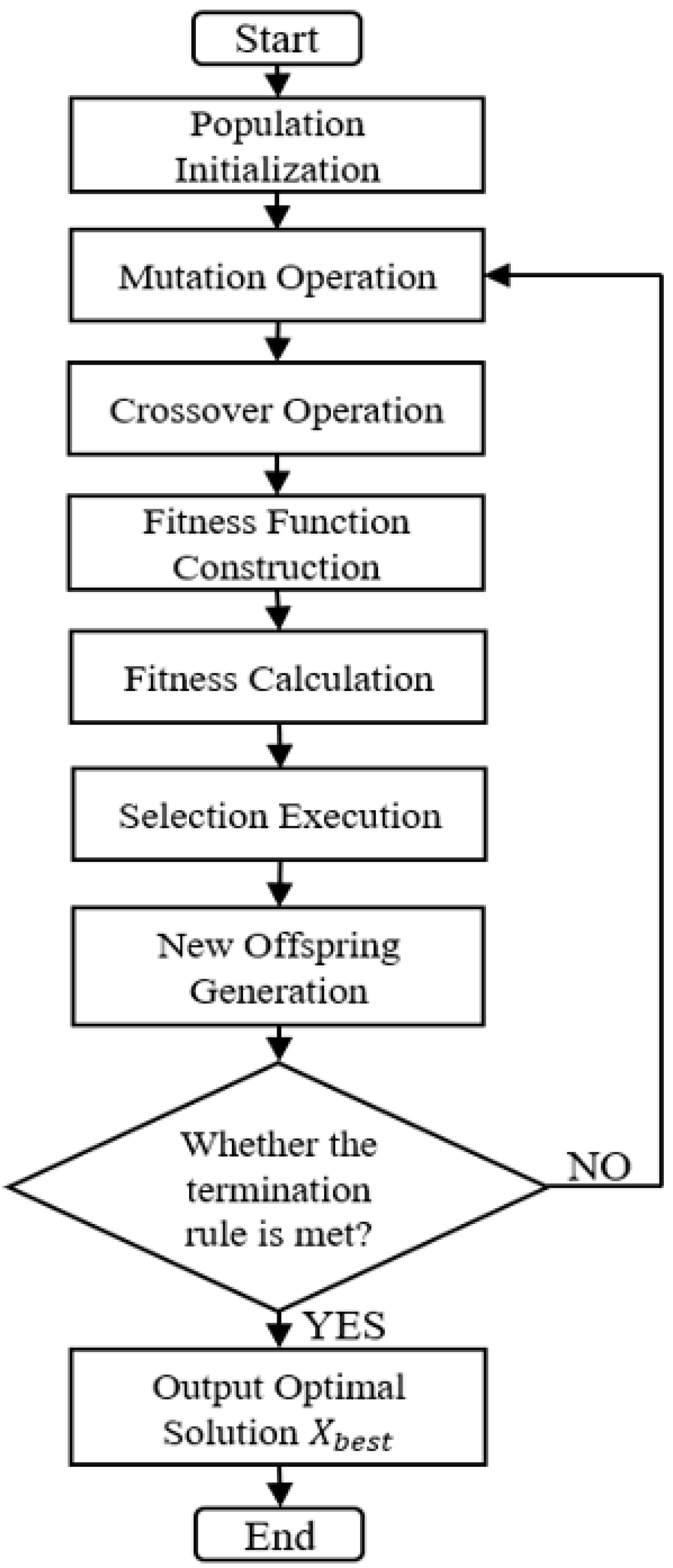
A differential evolution algorithm suitable for high-dimensional decision vector optimization problems is adopted in the paper in order to seek an optimal solution to the system energy consumption for the parallel configuration of different types of pumps [16]. The parameters to be optimized in the PVFPS include the number of different types of pumps (integer variable) and the speed regulation rate (real variable); however, there are still some deficiencies in deducing the optimal integer variables while using the DE [17]. Accordingly, the conventional DE needs to be modified and improved in order to adapt to this particular optimization problem. The flow chart of the improved DE algorithm is shown in Figure 2.

Assuming that the dimension of vector individual is D and the number of vector individuals is NP, consequently the vector individual in the population can be expressed as follows:

$$\mathrm{X}=\left(\mathrm{x}\left[0\right], \mathrm{x}\left[1\right],\dots , \mathrm{x}\left[\mathrm{D}\right]\right)$$

(9)

where integer variables and real variables are both included in it.

3.1. Population Initialization

The initialization of real variables for this particular algorithim is the same as for the conventional DE. Nevertheless, for the integer variables, the initialized variables should be rounded up. In this case, n₁ and n₂ are integer variables, while s is a real variable. Thus, the initial value of X can be defined as follows:

$${\mathrm{x}}_{\mathrm{i}, \mathrm{j}}=\mathrm{np}. \mathrm{round}\left(\mathrm{random}. \mathrm{uniform}\left(0, 1\right) \left({\mathrm{x}}_{\mathrm{j}}^{\max }-{ \mathrm{x}}_{\mathrm{j}}^{\min }\right){+\mathrm{x}}_{\mathrm{j}}^{\min }\right) \left(\mathrm{j}=0, 1\right)$$

(10)

$${\mathrm{x}}_{\mathrm{i}, \mathrm{j} }=\mathrm{random}. \mathrm{uniform}\left(0, 1\right) \left({\mathrm{x}}_{\mathrm{j}}^{\max }-{ \mathrm{x}}_{\mathrm{j}}^{\min }\right){+\mathrm{x}}_{\mathrm{j}}^{\min } \left(\mathrm{j}=2\right)$$

(11)

where ${\mathrm{x}}_{\mathrm{i}, \mathrm{j}}$ represents Ihe jth dimensional parameter of the ith vector individual in the initial generation population; ${\mathrm{x}}_{\mathrm{j}}^{\max }$ and ${ \mathrm{X}}_{\mathrm{j}}^{\min }$ are the upper and lower bounds of parameter variables, respectively; and random. uniform(0, 1) indicates random real numbers on the [0, 1] interval, and np. round in Equation (10) means rounding to the nearest integral number.

3.2. Mutation Operation

Mutation operation is the crucial procedure in the DE algorithm. For each target vector individual X_i(G) of the Gth generation population, two mutant vector individuals are to be formed by the DE/rand to best/1 strategy shown as the following equations [18]:

$${\mathrm{v}}_{\mathrm{i}, \mathrm{j}}=\mathrm{math}. \mathrm{ceil}\left({\mathrm{x}}_{\mathrm{i}, \mathrm{j} }+\mathrm{F} \left({\mathrm{x}}_{\mathrm{best}}-{ \mathrm{x}}_{\mathrm{r}3}\right)+\mathrm{F} \left({\mathrm{x}}_{\mathrm{r}1}-{ \mathrm{x}}_{\mathrm{r}2}\right)\right) \left(\mathrm{j}=0, 1\right)$$

(12)

$${\mathrm{v}}_{\mathrm{i}, \mathrm{j}}=\left({\mathrm{x}}_{\mathrm{i}, \mathrm{j} }+\mathrm{F} \left({\mathrm{x}}_{\mathrm{best} }-{ \mathrm{x}}_{\mathrm{r}3}\right)+\mathrm{F} \left({\mathrm{x}}_{\mathrm{r}1}-{ \mathrm{x}}_{\mathrm{r}2}\right)\right) \left(\mathrm{j}=2\right)$$

(13)

where v_i,j is the mutant vector individual; x_best is the optimal vector individual of the current generation; and x_r1, x_r2 and x_r3 are three randomly selected vector individuals, in which i, r1, r2 and r3 are different from each other; the Fs are the scaling factors of mutation operation. Additionally, math. ceil in Equation (12) means rounding up, in order to meet the hydraulic demand of the pumping station.

In order to maintain the diversity of populations and avoid the destruction of the optimal solution simultaneously, we define the following:

$${\mathsf{\lambda }=\mathrm{e}}^{1 -\frac{{\mathrm{G}}_{\mathrm{t}}}{{\mathrm{G}}_{\mathrm{t}}+1 - \mathrm{G}}}{, \mathrm{F}=\mathrm{F}}_0{ \times 2}^{\mathsf{\lambda }}$$

(14)

where G–is the current number of iterations and G_t is the termination generation; the value of F₀ is taken to be 0.5 in this case.

3.3. Crossover Operation

The goal of the crossover operation is to generate individual test vectors, in order to further increase the diversity of interference parameter vectors and consequently improve the differential mutation search strategy. The detailed crossover operation is represented as follows [19]:

$${\mathrm{u}}_{\mathrm{i}, \mathrm{j}}=\left\{\begin{array}{c}{ \mathrm{v}}_{\mathrm{i}, \mathrm{j}}, \mathrm{rand}\left(0, 1\right) \le { \mathrm{CR} \mathrm{or} \mathrm{j}=\mathrm{j}}_{\mathrm{rand}}\\ { \mathrm{x}}_{\mathrm{i}, \mathrm{j}}, \mathrm{rand}\left(0, 1\right) > \mathrm{CR} \mathrm{and} \mathrm{j} \ne { \mathrm{j}}_{\mathrm{rand}}\end{array}\right.$$

(15)

If rand(0, 1) is less than or equal to CR, the value source of the test individual inherited from mutant vector v_i,j, otherwise duplicates ${ \mathrm{x}}_{\mathrm{i}, \mathrm{j}}$. In addition, j_rand is the randomly selected integer sequence number in [0, D], which is introduced to ensure that at least one dimension of the test vector individual is inherited from the mutant vector. CR $\in$ [0, 1] is the crossover rate, whose value has an influence on the population diversity and the convergence rate. When the value of CR is large, the mutant individual contributes more to the test vector individual, and the convergence rate is fast. On the contrary, the test vector individual inherits a large proportion from objective individual, and the population diversity is relatively rich. In order to guarantee the population diversity at the preliminary stage and the convergence rate at the later stage of the optimization process, a time-varying crossover rate CR is defined as follows:

$$\mathrm{CR}\left(\mathrm{G}\right){=\mathrm{CR}}_{\min }+\frac{{\mathrm{CR}}_{\max }-{ \mathrm{CR}}_{\min }}{\sqrt{{\mathrm{G}}_{\mathrm{t} }- \mathrm{G}+1}}$$

(16)

where CR_min and CR_max are the maximum and minimum crossover rates, respectively.

3.4. Fitness Function

Establishment of the fitness function should be combined with the objective function and constraints previously proposed above. When the constraints are handled, the commonly used methods include the repair method, variable elimination method, penalty function method and so on, among which the penalty function method is the most effective. A penalty factor can be applied on each constraint, in order to build an augmented objective function. The penalty function of the total flow constraint is shown in Equation (17), and the penalty function of the speed regulation ratio constraint is shown in Equation (18):

$${\mathsf{\delta }}_{\mathrm{Q}}=\left\{\begin{array}{c} 0, \hspace{1em}\mathrm{Q} \ge { \mathrm{Q}}_{\mathrm{t}}\\ \left|\mathrm{Q} -{ \mathrm{Q}}_{\mathrm{t}}\right|{, \mathrm{Q} < \mathrm{Q}}_{\mathrm{t}} \end{array}\right.$$

(17)

$${\mathsf{\delta }}_{\mathrm{s}}=\left\{\begin{array}{c} 0.5 - \mathrm{s}, \hspace{1em}\mathrm{s} < 0.5\\ 0, \hspace{1em}0.5 \le \mathrm{s} \le 1 \\ \mathrm{s} - 1, \hspace{1em}\mathrm{s} > 1\end{array}\right.$$

(18)

Taking ω and θ as the penalty factors, the final fitness function can be obtained as follows:

$$\mathrm{minF}\left({\mathrm{X}}_{\mathrm{i}}\left(\mathrm{G}\right)\right){=\mathrm{minJ}+\mathsf{\omega }\mathsf{\delta }}_{\mathrm{Q}}{+\mathsf{\theta }\mathsf{\delta }}_{\mathrm{s}}$$

(19)

3.5. Selection Execution

In order to determine whether the test vector individual will become a member of the next generation population, U_i(G + 1) is compared with X_i(G + 1) to evaluate the fitness of each individual; the vector individual that is retained makes the final fitness function have a smaller value. Subsequently, the new offspring generation is iterated through to obtain the fitness of each individual. The optimal vector individual X_best which has the best fitness shall be documented in each generation.

The loop iteration will not end until it reaches the maximum number of iterations, G_t, or until it meets the required accuracy of the solution. In the termination generation population, the final optimization solution is bound to be the vector individual that has the optimal value of the final fitness function.

4. Results of Algorithm Implementation

According to the energy consumption model in Equation (8), the objective variables to be optimized include the number of constant speed pumps (n₁), the number of speed regulating pumps (n₂) and the speed regulation rate (s). Hence, the ith vector individual of the Gth generation, whose dimension is three, can be defined as follows:

$${\mathrm{X}}_{\mathrm{i}}\left(\mathrm{G}\right)=\left({\mathrm{n}}_1\left(\mathrm{i}\right){, \mathrm{n}}_2\left(\mathrm{i}\right), \mathrm{s}\left(\mathrm{i}\right)\right) \left(\mathrm{i}=1, 2,\dots , \mathrm{NP}\right)$$

(20)

In summary, the optimization problem can be described as finding the point that minimizes the value of the final fitness function (Equation (19)) during the process of iterative evolution by using the improved DE algorithm.

Before using the improved DE algorithm to commence optimization in PyCharm, several input variables which exert an influence on the optimization range and speed still need to be assigned, in order to find the X_best rapidly and accurately. We define the dimension of vector individual as D = 3, the number of vector individuals as NP = 50 and the termination generation to be G_t = 300; Meanwhile, F and CR vary as the number of iterations increases.

After implementing the program, the optimal vector individual X_best is obtained, and part of the iterative optimization process is shown in Figure 3.

The simulation test used in this section is based on the pump design parameters and water supply targets collected on a certain day from a water circulation pumping station in an aluminum factory. The results of the improved DE algorithm optimization are shown in

Table 1. Part of the results from the improved DE algorithm optimization process.

Serial Number	Ht (m)	Qt (m3/h)	n1	n2	s	Min J (kW)	Solving Time (s)
1	56.7	8200	2	2	0.9781	1446.21	27.33
2	54.4	7530	2	2	0.9603	1259.62	28.01
3	48.7	5530	1	2	0.8927	813.88	27.28
4	43.1	2200	0	2	0.8289	263.13	28.23

. For the sake of comparison, the results of genetic algorithm (GA) optimization [20] are shown in

Table 2. Part of the results from the GA optimization process.

Serial Number	Ht (m)	Qt (m3/h)	n′1	n′2	s′	Min J′ (kW)	Solving Time (s)
1	56.7	8200	1.99	2.00	0.9911	1535.09	51.07
2	54.4	7530	1.50	1.99	0.9735	1388.37	50.48
3	48.7	5530	0.60	1.97	0.9356	910.12	49.59
4	43.1	2200	0.03	1.60	0.8707	324.82	52.11

.

5. Experimental Testing and Verification

In this tested system, the water circulation pumping station consists of five centrifugal pumps of two types, whose configuration parameters are shown in

Table 3. Design parameters and characteristics of the pump unit.

Serial Number	Model Type	Design Head (m)	Design Flow (m3/h)	Rotation Rate (r/min)	Virtual Head Coefficient (Hx)	Virtual Impedance Coefficient (Sx)
1	20SA-10	58	2850	960	70.39	1.78 × 10−6
2	20SA-10	58	2850	960	70.39	1.78 × 10−6
3	20SA-10	58	2850	960	70.39	1.78 × 10−6
4	14SH-9B	58	1425	1450	71.17	7.48 × 10−6
5	14SH-9B	58	1425	1450	71.17	7.48 × 10−6

. Among them, pump No. 4 and pump No. 5 are speed regulating pumps. The pumping station site is shown in Figure 4. It is an essential facility in the production process of an aluminum industry company.

After retrieving relevant data records, the water supply demands of the pumping station throughout a certain day are shown in Figure 5. Meanwhile, the annual water consumption pattern and annual water consumption statistics of the pumping station are illustrated in Figure 6 and Figure 7.

According to the process analysis, the pressure values of the system need to be maintained during the evaporation process flow. The vertical height H₀ of the evaporator to the water surface of the pump sump is about 22 m, and the working pressure of the evaporator is 0.2 MPa. Hence, the pump system must overcome piping losses from the evaporation process and pressure of at least 0.42 MPa. The actual hydraulic demand curve of the system is shown in Figure 8.

Before using frequency converters, the system was just adjusted by using valves. Compared to using a parallel variable frequency pump system (PVFPS), using valves was energy-intensive and electricity-consuming. According to the strategy in Section 3, the scheduling function for minimum shaft power is established, and the improved DE algorithm is implemented to solve for the optimal value of shaft power within the working flow region. The optimization scheduling algorithm is embedded in the cloud computing module of DG-IoT, which is a lightweight open-source platform for industrial IoT. The cloud platform sends command signals to the operation control circuits after completing the calculation in a short time. The circuit board communicates with the cloud platform via wireless network, and the MCU of the board is able to process command signals to further control the operation of the PVFPS. The results of shaft power in different configurations are shown in Figure 9.

Based on the annual water consumption data in Figure 7 and the shaft power data in Figure 9, the annual energy consumption can be calculated. Assuming that the electricity price is $0.1/kWh, the annual electricity savings can also be estimated. The results are shown in

Table 4. Annual energy consumption and estimated annual electricity savings of the pumping station.

Configuration	Annual Energy Consumption (kWh)	Annual Energy Saving (kWh)	Saving Rate (%)	Electricity Fees (Million Dollars)	Money Saving (Million Dollars)
Original	9,075,400	0	0	0.908	0
PVFPS	7,570,600	1,504,800	16.6	0.757	0.151

.

6. Conclusions

In this paper, an energy-saving strategy applied to a PVFPS was proposed. Subsequently, the shaft power model of the PVFPS was built and the DE algorithm was improved and used to solve for the optimal number of pumps in operation as well as the optimal speed regulation rate. By contrast, the GA was also introduced to solve the same problem. In the end, a test was conducted to verify the applicability and energy-saving effect of the improved DE algorithm in a real pumping station case. The following conclusions can be drawn:

(1)

The best solutions, including the optimal number of different pumps in operation, speed regulation ratio and solution time, solved by the improved DE algorithm and GA are exhibited, respectively, in Section 4. In comparison, the optimization objective J that was optimized by the improved DE averaged 9.68% smaller than J’ optimized by the GA. Moreover, DE costs less solving time (an approximately 20-second difference) and requires much fewer iterations to find the global optimal solution than GA. It is also worth mentioning that the optimal number of different pumps in operation is returned as an integer in DE, but not a real number in GA, as a result of the improvements provided by the DE algorithm.

(2)

The improved DE algorithm is designed into a cloud computing module of a pump operation control platform, and the optimization process was successfully realized in a real site to regulate and control a PVFPS. Compared with the original configuration without an intelligent scheduling algorithm, a PVFPS saves 16.6% in electricity consumption and 0.151 million dollars annually, which verifies the feasibility and economy of the improved differential evolution algorithm applied as an energy saving strategy to a parallel variable frequency pump system.

(3)

Further research will address the operation and maintenance costs of the whole pump system in order to decrease the wear and tear of pumps, improve the reliability of the system and reduce the impact on the surrounding environment.