Planning of Flexible Generators and Energy Storages under High Penetration of Renewable Power in Taiwan Power System

Abstract

The proportion of renewable power generation in the world has been increasing in recent years. However, the fluctuations and uncertainties of renewable power generation bring a considerable challenge to future unit scheduling. Therefore, the generation flexibility in power systems becomes more critical as a large amount of renewable generation is integrated into power systems. The use of flexible generators with energy storage systems is one of the most efficient methods of improving power system flexibility. The primary purpose of this study is to explore the effect of generation flexibility on the cost of unit scheduling. A flexibility index is used to evaluate the generation flexibility in the Taiwan power system, and a multi-scenario analysis for renewable power integration is considered. This study also considers various system constraints, such as the unit commitment of actual hydro and thermal units, the scheduling of flexible internal combustion engines (ICEs) and energy storage systems, and possible curtailments of renewable power generation. According to the seasonable characteristics of renewable power generation, this study provides a suitable capacity for flexible ICE units and energy storage systems. Furthermore, this study demonstrates that the cost of unit scheduling is effectively reduced by increasing flexible ICE units and energy storage systems. The results of this study can be used as a reference for power systems in preparing flexible generating units and energy storage systems under the integration of a large amount of renewable power generation in the future.

1. Introduction

The integration of renewable power generation into power grids brings significant challenges to unit scheduling. Thus, power systems need more generation flexibility to maintain grid reliability. In addition, replacing large-scale conventional units with renewable energy reduces power system inertia and increases the need for ramping capability and operating reserve, specifically, load-following services [1]. Many studies were related to the flexibility of an electrical system and quantified it. B. Mohandes et al. [1] reviewed various indices that are commonly used in the literature to express power system flexibility, which covers ramping limit, power capacity, and energy capacity. Furthermore, Y. K. Wu et al. [2] quantified the flexibility of a power system with analytic hierarchy process method and considered flexible generation units in unit scheduling problems. F. Pourahmadi et al. [3] studied the impact of wind generation temporal correlation on power system flexibility and the uncertainty interval of wind generation. M. Ghaljehei et al. [4] proposed an incentive for generation flexible ramping product in 15 min market, on top of the existing day-ahead flexible ramping market. The results show that the proposed incentive improves the reliability of the system and reduces the dependency on fast start generation.

In addition to generation side, many studies have also discussed the improvement of power system flexibility by using energy storage, electric vehicles, etc. [5,6,7,8,9,10,11]. M. Khoshjahan et al. [6,7] proposed a real-time price-based stochastic unit scheduling, where energy storage, e.g., pumped-hydro storage, can be modelled as a flexible ramping product, to reduce the impact of renewable energy fluctuations on power systems. A. Nikoobakht [8] proposed a generic continuous-time risk-based model for sub-hourly scheduling of generating units and energy storage, which ensures that the flexible resources track and compensate the sub-hourly variations of wind power generation. H. Li et al. [9] incorporated various flexibility resources, which entails generation units, load shedding, demand response, pumped hydro, battery storage, and compressed air storage, in a 213-bus system for power system flexibility study. Numerical results suggested that energy storage is preferred for operation optimization, and a power system should install a certain amount of storage capacity to deal with the uncertainty of renewable energy generation. A. A. Lekvan et al. [10] presented a hybrid robust/stochastic scheduling for multi-energy microgrid, which incorporates electric vehicle parking lots, power-to-gas facility, and demand response, to cope with renewable generation uncertainty. Y. Yuan et al. [11] presented a renewable and storage planning model considering the retirement of coal plants, carbon policy and storage price. However, a deterministic model is implemented that does not consider the uncertainty from the renewable energy resources. X. Y. Chenet al. [12] defined generation flexibility as ramping capability, minimum power output, minimum online/offline time, etc., and indicated that energy storages or ICEs can provide a significant grid flexibility because they can start up and generate their full capacity in a few minutes. That is, they have the advantages of rapid ramping rates and low minimum generation. Furthermore, ICEs can flexibly provide different generation capacities through modularization, increasing the range and reliability of generation regulation [13,14].

Many stochastic variables can be used in decision planning, especially in an intermittent generation environment, which brings more significant challenges to unit scheduling. W.S. Tan et al. [15] reviewed various stochastic unit scheduling models, where incorporation of power system flexibility is thoroughly discussed. It is also mentioned that the integration of a large amount of renewable energy should consider various generation scenarios, but at the same time reduce the number of scenarios appropriately to preserve computational tractability while retaining the probability distribution of each representative scenario [6,16]. E. Du et al. [17] considered multi-scenario modeling of renewable power generation, and each scenario represents uncertainties and corresponding probability distributions. The scenarios were generated using historical data with Monte Carlo simulation.

Based on the above discussion, it is summarized that generation flexibility becomes more important owing to a large amount of renewable energy integration. Therefore, this study aims to investigate the impact of high penetration of renewable generation to future Taiwan’s power system and explore possible mitigation strategies, for instance, via the inclusion of flexible ICEs and energy storage in the grid to improve generation flexibility. ICE is a more flexible power resource compared to traditional combined cycle gas turbines or open cycle gas turbines. A flexible generation can ramp up/down rapidly and operate at a low output. Furthermore, multiple small ICEs can be connected in parallel to scale up the total power output as desired. The contributions of this paper are outlined as follows:

(1)

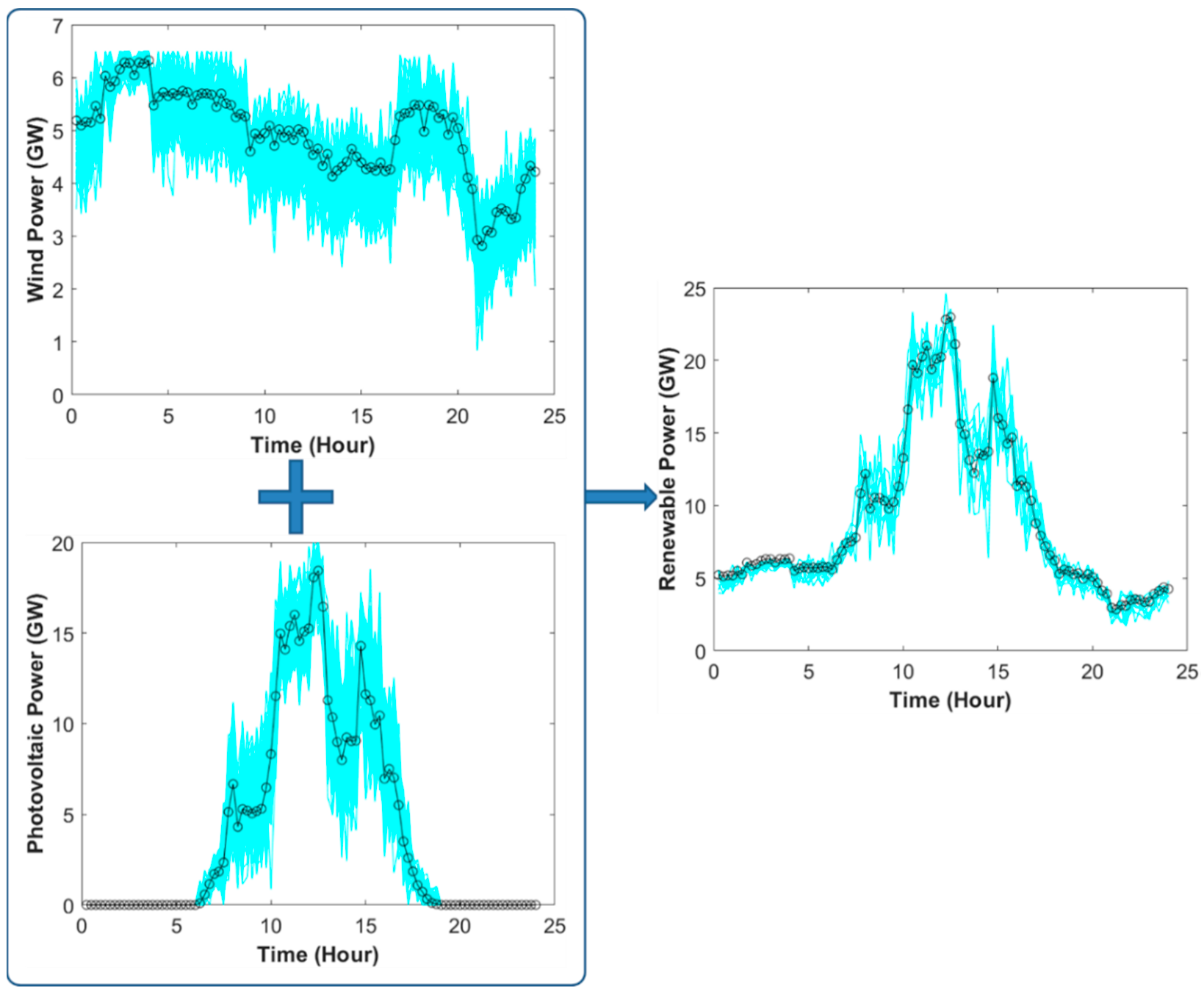
A Taiwan power grid with realistic renewable energy generation is modeled as a stochastic unit scheduling problem. Resources covering all the generation, load demand, pumped storage, hydro generation, future flexible ICEs, and energy storage installations are included. This system allows researchers to comprehensively explore the effect of generation flexibility on the future Taiwan power grid, especially for the operating cost of unit scheduling.

(2)

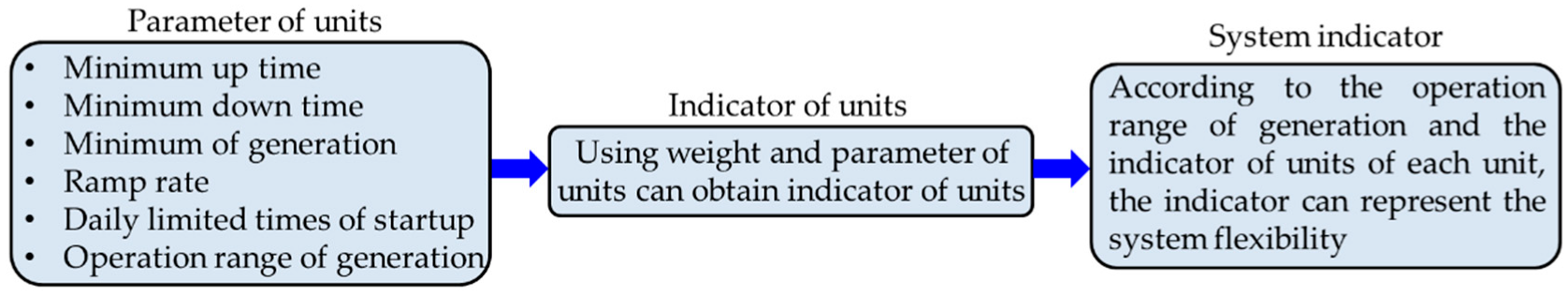
Flexible ICEs and energy storages are considered as potential resources to provide generation flexibility, and the flexibility index is quantified by utilizing the fuzzy analytic hierarchy process method.

(3)

Sensitivity analysis has been simulated with four seasons that have different scenarios for renewable power generation. It provides a comprehensive study of the effect of generation flexibility on the operation cost of unit scheduling.

(4)

Lastly, in conjunction with the growth in generation flexibility, the proposed framework manages to precisely identify the appropriate and optimal capacities for flexible ICEs and energy storage installations, which is essential for future Taiwan power system planning.

The main purpose of this study is to present a comprehensive Taiwan power grid with realistic renewable energy generation, which is modelled as a stochastic unit scheduling problem. Resources covering all the generation, load demand, pumped storage, hydro generation, future flexible ICEs, and energy storage installation are included. This system allows researchers to comprehensively explore the effect of power system flexibility on the future Taiwan power grid.

2. Renewable Energy Efforts in Various Contexts

Unit scheduling must consider multi-scenarios of renewable power generation. In this study, the renewable-energy data were scaled up from real-time measurements in Penghu to a total capacity of 20 GW solar power and 6.5 GW wind power. Additionally, renewable energy forecasting errors provided by Elia, a Belgian high voltage power transmission system operator [18], were used to model the uncertainty of renewable power generation. The steps for generating multi-scenarios are as follows: First, the data on Elia’s website are divided by two types of renewable energy (wind and solar) and seasons, and the data are normalized and divided into multiple intervals, for every 10% increment of the generation capacity. Second, the forecasting errors with corresponding probability distributions for wind and solar power are obtained for each season. Figure 1 and Figure 2 demonstrate the distribution of forecasting errors in the first interval for solar and wind power in spring, respectively. The first interval indicates the power generation between 0% and 10% of the total generation capacity.

Furthermore, the next step is the generation of Taiwan’s renewable energy scenarios. The historical renewable energy generation data (wind and solar) from Taiwan will be subtracted with the random values extracted from the corresponding probability distribution function of the renewable energy forecast error to generate 100 scenarios, since it is sufficient to represent the distribution of renewable power generation (wind and solar). Each scenario consists of 96 intervals in a day, with 15 min per timestep. Next, all the generated wind and solar scenarios are summed up to create 100 scenarios of combined renewable power generation. Then, the Scenario Reduction Backward Method (SRBM) of General Algebraic Modeling System (GAMS) software [19] was used to transfer the 100 multi-scenarios into 10 renewable energy scenarios with different probabilities, as shown in Figure 3. The use of 10 resultant scenarios is in line with other stochastic unit scheduling model in the literature [6]. Using low number of scenarios will maintain the computation tractability of the unit scheduling model. In the process of scenario reduction, if a scenario is close to another scenario or has a low probability of occurrence, it will be deleted [19].

In this paper, a total installed capacity of renewable power sources is set according to the future Taiwan’s energy policy. By 2025, Taiwan is expected to install about 20 GW solar power capacity and 6.5 GW wind power capacity.

3. Calculation of Flexible Indexes

Power system flexibility can be specifically quantified using various metrics. Among them, the fuzzy analytic hierarchy process (FAHP) and analytic hierarchy process (AHP) have been widely used in multi-conditional judgment issues [20,21]. AHP is used for decision-making in uncertain problems. The power industry often applies AHP metrics for reliability assessments or maintenance procedures of plants. However, A. Ishizaka et al. [22] revealed that AHP may not be able to judge human subjectivity when expert evaluations are converted into values, but FAHP could provide more objective evaluation. Thus, this study uses FAHP to evaluate power generation flexibility.

Estimation of power generation flexibility usually considers minimum up time/minimum down time, ramp-up rate/ramp-down rate, minimum output of the generator, operating range, and the unit’s start-up/shut-down times. This study uses the above variables and the FAHP method to calculate the flexible index of each generator. Since the flexibility variables at each generator have different units and ratios, these variables are normalized by normalization process, which considers the positive and negative correlation to the overall system flexibility, which is expressed as follows:

$$I=\frac{x-bas{e}_{min}}{bas{e}_{max}-bas{e}_{min}},$$

(1)

$$I=1-\frac{x-bas{e}_{min}}{bas{e}_{max}-bas{e}_{min}},$$

(2)

where I is the value after normalization, x is one of the variables at a unit, and $bas{e}_{max}$ and $bas{e}_{min}$ are the maximum value and the minimum value at each variable, respectively.

To specify the contribution of each variable to the overall flexibility in the system, it is necessary to assign an appropriate weight to each variable, which was obtained through an expert questionnaire. Based on the recommendations of 10 experts in the field of power systems, the weight matrix of the FAHP method was constructed, and the parameters of each unit with a corresponding weight matrix were used to calculate the flexibility of both generators and the whole power system. Figure 4 illustrates how to calculate the flexibility index of the overall system by the FAHP method, which is well discussed in [2].

4. Unit Scheduling and Economic Dispatch

4.1. Stochastic Unit Scheduling

Stochastic unit scheduling is a typical mathematical optimization problem that aims to minimize generation cost under several technical constraints and uncertainties from renewable power generation. The objective function of stochastic unit scheduling consists of three components: fuel cost function of generation units, start-up cost, and penalty cost.

$$min {\sum }_{s=1}^{S}P{r}_s{\sum }_{t=1}^T{\sum }_{j=1}^J\left[C_{fuel}\left(P_{t,j,s}\right)+C_{StartUp}+C_{Penalty}\right],$$

(3)

where $P{r}_s$ is the probability for each scenario s, S is the total number of scenarios, P_t,j,s is the power generation from unit j and scenario s at time t, $C_{fuel}\left(P_{t,j,s}\right)$ is the fuel cost of unit j under scenario s at time t, $C_{StartUp}$ is the start-up cost of unit j and scenario s at time t, and $C_{Penalty}$ is the penalty cost (also called compensation cost), which is a relative cost for compensating power generation or reserve. Since there may be occasional shortfalls in unit capacity or operating reserve in realistic operations, it is necessary to assume a high penalty cost so that the unit scheduling program can still be eventually converged.

This study utilizes mixed-integer linear planning (MILP) for unit scheduling, which allows the fuel cost curve to be linearized using a segmented linearity approach. In addition, the proposed optimization problem contains the following constraints:

$$Pmi{n}_j<P_{t,j,s}<Pma{x}_j,$$

(4)

$$-o_{t-1,j,s}+o_{t,j,s}\le StartU{p}_{t,j,s},$$

(5)

$${\sum }_{j=1}^J{P}_{t,j,s}+P_{t,s}^{RE}-P_t^{cut}=Deman{d}_t^{total},$$

(6)

$${\sum }_{j=1}^{J}Reserv{e}_{t,j,s}^{up}=ReserveU{p}_{t,s}^{total},$$

(7)

$${\sum }_{j=1}^{J}Reserv{e}_{t,j,s}^{down}=ReserveDow{n}_{t,s}^{total},$$

(8)

$$ReserveU{p}_t^{total}\ge 0.01·Deman{d}_t^{total}+MaxGen+0.1·P_{RE}^t,$$

(9)

$$ReserveDow{n}_t^{total}\ge 0.01·Deman{d}_t^{total}+0.1·P_{RE}^t,$$

(10)

$$Tminu{p}_j\le {\sum }_t^{t+Tminu{p}_j}{o}_{t,j,s},$$

(11)

$$Tmindow{n}_j\le {\sum }_t^{t+Tmindow{n}_j}(1-o_{t,j,s}),$$

(12)

$$P_{t,j,s}-P_{t-1,j,s}\le RampU{p}_j,$$

(13)

$$P_{t-1,j,s}-P_{t,j,s}\le RampDow{n}_j,$$

(14)

$$P_{t,j,s}+Reserv{e}_{t,j,s}^{up}-P_{t-1,j,s}\le RampU{p}_j,$$

(15)

$$P_{t,j,s}-Reserv{e}_{t,j,s}^{down}-P_{t-1,j,s}\ge -RampDow{n}_j,$$

(16)

$$P_t^{cut}\le P_{t,s}^{RE},$$

(17)

where $Pmi{n}_j$ is the minimum output of unit j, $Pma{x}_j$ is the maximum output of unit j, $o_{t,j,s}$ is the state of unit j and scenario s at time t (binary variable), $StartU{p}_{t,j,s}$ is the state of start-up for unit j and scenario s at time t (binary variable), $P_{t,s}^{RE}$ is the renewable generation of scenario s at time t, $Deman{d}_t^{total}$ is the total system demand at time t, $Reserv{e}_{t,j,s}^{up}$ and $Reserv{e}_{t,j,s}^{down}$ are the upward and downward reserve from unit j and scenario s at time t, respectively, $ReserveU{p}_{t,s}^{total}$ and $ReserveDow{n}_{t,s}^{total}$ are the total upward and downward reserve requirement of scenario s at time t, respectively, $Tminu{p}_j$ and $Tmindow{n}_j$ are the minimum up and down time of unit j, respectively, $RampU{p}_j$ and $RampDow{n}_j$ are the generation ramp up and down rate of unit j, respectively, and $P_t^{cut}$ is the renewable energy curtailment at time t.

Equation (4) is used to limit the generation range at each unit. Equation (5) determines the status of each unit’s start up. Equation (6) shows that a total power generation from conventional and renewable generation is equal to system load. Equations (7)–(10) consider the limitation of operating reserve. Equations (11) and (12) limit the minimum uptime and downtime at each unit, respectively. Equations (13) and (14) consider the limits of ramp up rate and ramp down rate, respectively. Equations (15) and (16) aim to limit the operating reserve at each unit. Equation (17) limits the amount of renewable energy curtailment.

A Combined Cycle Gas Turbine (CCGT) is composed of multiple gas turbine units and one steam turbine. The simulations in this study include 2 + 1 and 3 + 1 types of CCGT combinations. Each CCGT unit has various operating modes, and its minimum start-up time and downtime must be considered when the output of a CCGT unit is increased or decreased.

Except for thermal power units, this study also considers hydraulic power units with pumped storage, including the six pumped storage units at Mingtan Power Plant and the four pumped storage units at Guanji Power Plant, with the following constraints:

$$Pmi{n}_{m,s}^{pp}·e_{t,m,s}^{pp}\le E_{t,m,s}^{pp}\le Pma{x}_{m,s}^{pp}·e_{t,m,s}^{pp},$$

(18)

$$Pmi{n}_{m,s}^{gp}·e_{t,m,s}^{gp}\le E_{t,m,s}^{gp}\le Pma{x}_{m,s}^{gp}·e_{t,m,s}^{gp},$$

(19)

$$e_{t,m,s}^{pp}+e_{t,m,s}^{gp}+e_{t,m,s}^{ideal}\le 1,$$

(20)

$$U_{t,m,s}^{pp}+U_{t,m,s}^{gp}\le 1,$$

(21)

$$LowRes{ }_{t,s}=LowRes{ }_{t-1,s}+{\sum }_{gp}\frac{E_{t-1,s}^{gp}}{EW{R}_{ }}-{\sum }_{pp}\frac{E_{t-1,s}^{pp}}{\left(\frac{EWR}{Eff}\right)},$$

(22)

$$WaterLeve{l}_{0,s}=WaterLeve{l}_{T,s},$$

(23)

$$Re{s}_{min}\le LowRes{ }_{t,s}\le Re{s}_{max},$$

(24)

where $Pmi{n}_{m,s}^{pp}$ and $Pma{x}_{m,s}^{pp}$ are the minimum and maximum power during pumping operation of the pumped storage m and scenario s, respectively, $Pmi{n}_{m,s}^{gp}$ and $Pma{x}_{m,s}^{gp}$ are the minimum and maximum power during generation operation of the pumped storage m and scenario s, respectively, $e_{t,m,s}^{pp}$, $e_{t,m,s}^{gp}$, and $e_{t,m,s}^{ideal}$ are the binary variable that determines the operation status (pumping, generation, or idle) of the pumped storage m and scenario s at time t, respectively, $E_{t,m,s}^{pp}$ and $E_{t,m,s}^{gp}$ are the pumping and generation power of the pumped storage m and scenario s at time t, respectively, $U_{t,m,s}^{pp}$ and $U_{t,m,s}^{gp}$ are the binary variables that indicate the real-time operation of pumping or generating mode of the pumped storage m and scenario s at time t, respectively, $EWR$ is the power-to-water ratio, $Eff$ is the pumping efficiency, $LowRes{ }_{t,s}$ is the reservoir water level of scenario s at time t, $WaterLeve{l}_{t,s}$ is the lower pool water level of scenario s at time t, and $Re{s}_{min}$ and $Re{s}_{max}$ are the minimum and maximum reservoir water level, respectively.

Equations (18) and (19) limit the pumping (storing energy) and generating capacity of a pumped storage unit, respectively. Equation (20) indicates that a single pump storage unit can contain three operating modes: pumping, generation, or idle. Equation (21) indicates that a unit can only operate in either pumping or generating mode. Equation (22) calculates the water level in the lower pool, and this constraint considers the power-to-water ratio and the pumping efficiency. The power-to-water ratio is defined as the ratio of power generation to the water consumption of the pumped storage units. The pumping efficiency describes the energy loss in the pumping process. Equation (23) sets that the water level at the first hour is the same as that at the last hour on each day, and Equation (24) limits the water level of the reservoir.

4.2. Economic Dispatch

In this study, economic dispatch is implemented based on a 15-min interval to account for short-term changes in renewable energy and load. After the unit scheduling procedure introduced in the previous section, the on/off status of thermal and hydroelectric units are decided at each hour. However, the on/off status of both ICE flexible units and energy storage systems is rescheduled to increase system flexibility. In this study, energy storage is only considered for economic dispatch every 15 min throughout the day because Taipower utilizes the energy storage system as a 15-min frequency regulation tool. The relevant objective function and constraints are as follows:

Objective function:

$$min{\sum }_{s=1}^{S}P{r}_s{\sum }_{t=1}^{t=96}{\sum }_{i=1}^I\left[\left(ChargeCost·E{S}_{t,i,s}^{ch}+DischargeCost·E{S}_{t,i,s}^{disch}\right)/4\right],$$

(25)

Limitation equation:

$$Pmi{n}_i^{disch}·e_{t,i,s}{\le }_{}E{S}_{t,i,s}^{disch}\le Pma{x}_i^{disch}{}_{ }·e_{t,i,s},$$

(26)

$$Pmi{n}_i^{ch}{}_{ }·\left(1-e_{t,i,s}\right){\le }_{ }E{S}_{t,i,s}^{ch}\le Pma{x}_i^{ch}·\left(1-e_{t,i,s}\right),$$

(27)

$$So{C}_{t,i,s}=So{C}_{t-1,i,s}+[{\eta }_i^{ch}·E{S}_{t,i,s}^{ch}-(1/{\eta }_i^{disch})·E{S}_{t,i,s}^{disch}]·(1/E{S}_i^{max}),$$

(28)

$$E{S}_i^{min}/E{S}_i^{max}\le So{C}_{t,i,s}\le 1,$$

(29)

$$So{C}_{T,i,s}\le 75\%,$$

(30)

where $E{S}_{t,i,s}^{ch}$ and $E{S}_{t,i,s}^{disch}$ are the charging and discharging energy of i storage and scenario s at time t, respectively, $ChargeCost$ and $DischargeCost$ are the charging and discharging operation costs, respectively, $e_{t,i,s}$ is the binary variable that determines the charging or discharging status of i storage and scenario s at time t, ${\eta }_i^{ch}$, and ${\eta }_i^{disch}$ are the charging and discharging efficiency of i storage, respectively, $So{C}_{t,i,s}$ is the state of charge of i storage and scenario s at time t, and $E{S}_i^{min}$ and $E{S}_i^{max}$ are the minimum and maximum capacity of i storage, respectively.

Equation (25) is the objective function of dispatching energy storage system, whose goal is to minimize charging and discharging cost. Equations (26) and (27) limit the charging and discharging capacity of the energy storage device, respectively. Equations (28)–(30) show the limits related to the state of charge (SoC) of the energy storage system, which is assumed to be maintained at 75% of rated capacity in the last 15 min on each day. SoC is the charging level of a battery relative to its capacity. SoC is typically used to reveal the current state of a battery in use, and it also determines the lifetime of a battery. The ramp up/down rate and the demand/supply balance of the operating reserve from storage systems are subject to the same limitations as shown in Equations (13)–(16).

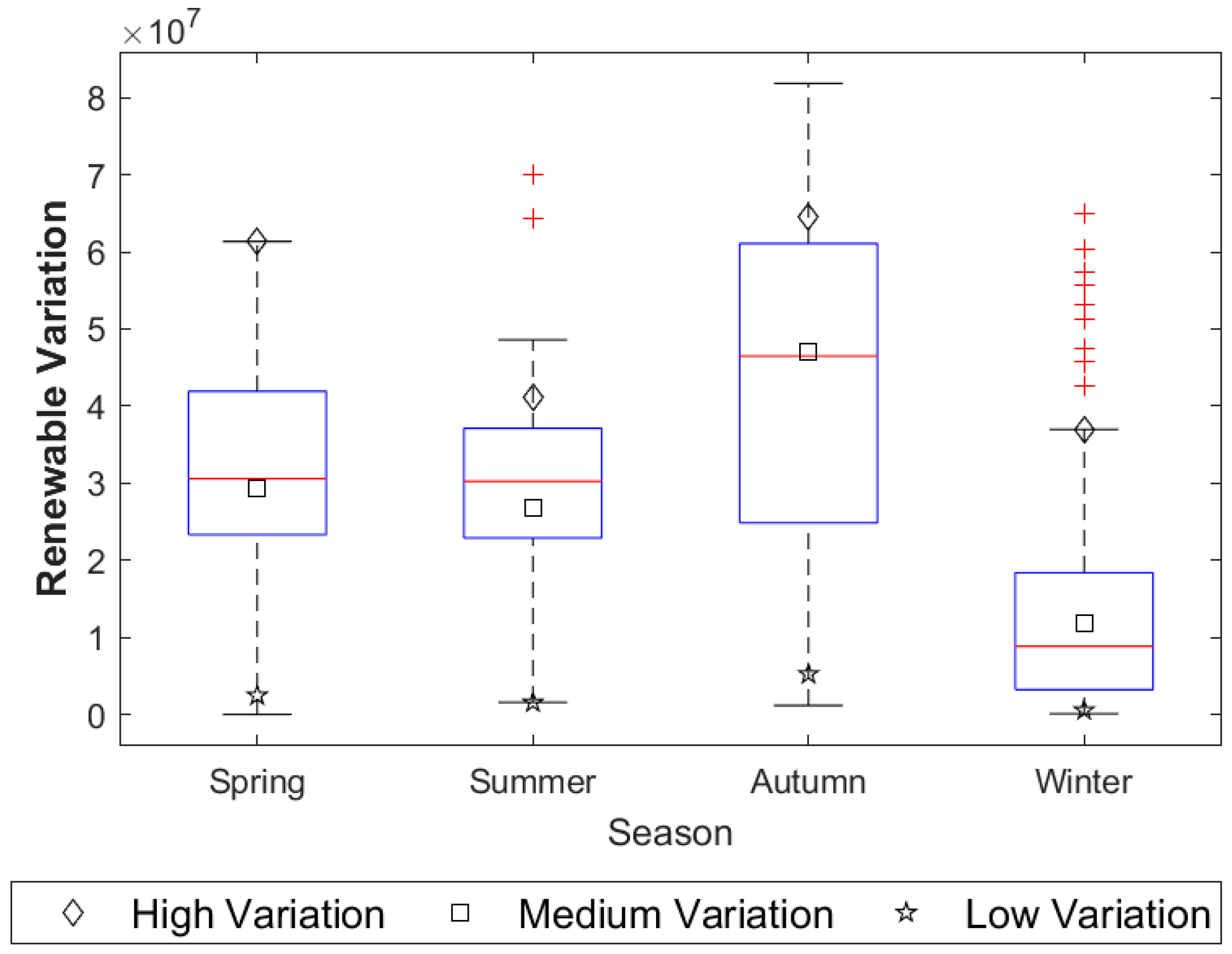
5. High Percentage of Renewable Energy Scenarios Analyzed and Simulated

In this study, new and decommissioned generating units of the Taipower system in 2025 are considered for unit scheduling, in which an installed capacity of 20 GW solar and 6.5 GW wind are integrated into Taipower. This study aims to analyze the impact of adding flexible units and energy storages on the cost of unit scheduling. Since the characteristics between renewable power generation and load demand are diverse in different seasons, this study has carried out unit scheduling in different seasons.

This study is divided into five different scenarios for ICE flexible unit combinations: the first scenario does not consider any flexible unit;

Table 1. Original case for generating units.

Unit Type	Single Unit Capacity (MW)	Number of Units
3 + 1 CCGT	720	25
3 + 1 CCGT	708	4
3 + 1 CCGT	428.7	5
2 + 1 CCGT	314.8	1
2 + 1 CCGT	273	3
Gas-fired	249	1
Gas-fired	537.88	1
Coal-fired	525	10

lists the original unit combinations in the analyzed system. In the second scenario, a total capacity of 720 MW conventional units is replaced by flexible ICEs. That is, a total capacity of 720 MW CCGT turbines is replaced by an equivalent capacity of ICEs (40 ICE units with 18 MW each). The third scenario is assumed to replace 1440 MW CCGT installed capacity by ICES with the same capacity. The fourth and fifth scenarios replace 2160 MW and 2880 MW CCGT capacity by ICEs, respectively. On the other hand, four energy storage scenarios, which include an installed capacity of 0 MWh, 500 MWh, 1 GWh, or 2 GWh, are considered in this study. In summary, a total of 200 scenarios (10 renewable power outputs, 4 different energy storage capacities, and 5 ICE flexible unit capacities) were considered for simulations.

Energy storage and ICE flexible units are the ones that we need to decide for future power system expansion planning. The selected ICE capacity is 18 MW per unit, while grid-connected energy storage is 500 MWh per unit. Forty ICE units are combined to form a 720 MW generation capacity to replace a unit of CCGT.

Most simulation parameters, such as the specifications of thermal generators in Taipower, are confidential. In general, different types of generators have different specifications. On the other hand, the simulation parameters of ICE flexible units are provided herein: the type of the chosen ICE is W18V50SG, produced by Wartsila company. The minimum continuous load of the generating set is 10% of its rated output, but the unit can still run on 0–10% load in a certain time period. There is no minimum run time for the generating set since it can be stopped immediately. The minimum downtime is about 3 min; then the unit can be ready for the next starting. The ramp up/down rate for a hot gas engine is 2.8% and 4% per second, respectively. Compared to combined cycle gas turbines or open cycle gas turbines, the ICE supports a more flexible power source to power systems because it has the capability of rapid startup and shutdown, a low minimum load, and a low minimum downtime. In terms of the energy storage, it is assumed that the charging or discharging rate of the battery is 500 MW/h, and the efficiency of battery charging and discharging is 95%. The SoC of the battery ranges between 0.1 and 1, and the cycle life of the battery is 4500. The above parameters are suggested by an ICE vendor.

Table 2. Relationship between ICE capacity and flexibility index under different unit combinations.

Unit Combination Case	Capacity of ICEs (MW)	Flexibility Index
1	0	0.4313
2	720	0.4454
3	1440	0.4588
4	2160	0.4716
5	2880	0.4839

shows the corresponding flexibility values that are calculated for different combinations of generating units. Obviously, the flexibility index varies according to different unit combinations. The larger the capacity of ICEs, the higher the flexibility index.

The simulations were carried out based on four seasons, and each season includes three scenarios: low, medium, and high, depending on the variability of renewable power generation. The probability values for renewable energy scenarios in four seasons and three variabilities are listed in

Table 3. Resultant scenarios probability implemented in various seasons and variation levels.

Season	Variation	Scenario
		1	2	3	4	5	6	7	8	9	10
Spring	Low	0.3	0.15	0.14	0.07	0.07	0.07	0.06	0.05	0.05	0.04
	Medium	0.21	0.14	0.13	0.1	0.09	0.09	0.08	0.07	0.05	0.04
	High	0.3	0.14	0.1	0.09	0.08	0.08	0.07	0.06	0.04	0.04
Summer	Low	0.28	0.22	0.21	0.09	0.07	0.04	0.03	0.03	0.02	0.01
	Medium	0.23	0.15	0.13	0.11	0.08	0.08	0.08	0.07	0.04	0.03
	High	0.18	0.15	0.13	0.12	0.12	0.1	0.08	0.08	0.03	0.01
Fall	Low	0.21	0.15	0.12	0.1	0.09	0.08	0.07	0.07	0.06	0.05
	Medium	0.2	0.17	0.17	0.14	0.11	0.07	0.05	0.04	0.03	0.02
	High	0.17	0.15	0.14	0.11	0.1	0.07	0.07	0.07	0.06	0.06
Winter	Low	0.22	0.18	0.18	0.14	0.09	0.06	0.05	0.03	0.03	0.02
	Medium	0.18	0.17	0.1	0.1	0.09	0.09	0.09	0.07	0.07	0.04
	High	0.17	0.13	0.13	0.1	0.1	0.09	0.09	0.08	0.06	0.05

in a descending arrangement. The box plot in Figure 5 shows the variation of renewable power generation during four seasons in a year, with the 25th percentile (Q1) and 75th percentile (Q3) at the top and bottom edges. The red horizontal line in the middle represents the median. The horizontal lines at the top and bottom of the box plot represent the maximum value within Q3 + 1.5 interquartile range (IQR) and the minimum value within Q1−1.5 IQR, where IQR = Q3 − Q1. The red “+” symbols indicate outliers. The box plots are used to select low, medium, and high variations of renewable power generation for each season. Three scenarios, below Q1, between Q1 and Q3, and above Q3, are selected. Obviously, the variability of renewable energy in Taiwan is highest in autumn. In contrast, the variation in summer and winter is smaller compared to other seasons.

5.1. Unit Scheduling in Spring

The study implemented unit scheduling in spring under the scenarios with low, medium, and high renewable-energy variability. Ten renewable power generation scenarios were included in this study. To simplify the demonstration, this paper only presents the analysis of the scenario with a “medium” level of variability from renewable power sources in spring. Figure 6 shows the 10 scenarios of net load in the spring. These scenarios were generated using the method introduced in Section 2. The results show that most net loads are close to zero in the midday period, but return sharply to the day’s peak towards the evening.

Based on the above net-load curves, a unit scheduling in the Taipower system was performed, where ICE flexible units and energy storage systems were also considered for scheduling to obtain operating cost. Figure 7 compares unit-scheduling costs according to different storage and ICE scenarios. This figure shows the total cost of all generating units. It is observed that an increase of ICE capacity significantly reduces unit-scheduling costs under a fixed storage capacity. For example, if the system has no storage, the cost of unit scheduling is reduced by 21.76%, 41.12%, 56.28%, and 61.28% when ICE capacity is increased by 0 MW, 720 MW, 1440 MW, 2160 MW, and 2880 MW, respectively. This reveals a significant contribution of ICE capacity to the unit-scheduling cost. On the other hand, an increase in storage capacity also affects the unit-scheduling cost. However, it is worth noting that in most of the scenarios, the maximum economic benefit is obtained as the storage capacity is 0.5 GW. That is, if the storage capacity is increased from 0.5 GW to 1 GW (or 2 GW), the contribution to cost reduction is not significant (less than 5%). Compared to 1 GW or 2 GW capacity, the storage capacity of 0.5 GW causes an efficient cost reduction. If increasing the storage capacity, the benefit of cost reduction will fade off.

Figure 8 shows the unit-scheduling results for 10 scenarios with different generation flexibility in spring. It means that the unit-scheduling cost for each scenario is multiplied by the occurrence probability of each scenario. Obviously, installing energy storages or replacing CCGTs with ICEs reduces the expected unit-scheduling cost.

5.2. Unit Scheduling in Summer

In summer, the characteristics of renewable power generation in Taiwan are low wind power but high solar power generation. To simplify the presentation, the analysis of the scenario with a “high” variability of renewable energy is demonstrated. Figure 9 shows the 10 sets of net-load curves for this scenario. The load demand is the highest in Taiwan during summer seasons, and the net-load curve is like a duck curve. Therefore, towards the evening a significant upward slope of the load demand is generated, leading to a shortage of upward operation reserves.

Figure 10 demonstrates the comparison of unit-scheduling costs in summer based on different storage and ICE scenarios. This figure illustrates the unit-scheduling costs after taking log₁₀. From the results, it is clear that increasing the capacity of flexible units reduces the average unit-scheduling cost. Furthermore, the installed capacity of storage also affects the unit-scheduling cost. Notably, compared to the capacity of 1 GW or 2 GW storage, the capacity of 0.5 GW of storage already significantly reduces the cost. The benefit of increasing more storage capacities for reducing unit-scheduling cost is not noticeable.

Figure 11 shows the relationship between unit-scheduling cost and generation flexibility in summer, where the unit-scheduling results for the 10 scenarios with the corresponding probability are considered. The results show that the unit-scheduling cost decreases as the flexibility index increases. Moreover, if the capacity of storage reaches up to 1 GW, an additional reduction of unit-scheduling cost is minimal. This means that the maximum economic benefit is achieved as the capacity of storage is 0.5 GW. Moreover, when the system has no flexible units, integrating an appropriate storage capacity on an appropriate time significantly benefits the unit scheduling.

In summer, if the variability of renewable power generation is high, the unit-scheduling costs become much higher compared to other variability scenarios; therefore, more ICE capacities are required. However, if the variability of renewable power generation is low, the system requires less flexible generation capacity. Nevertheless, the renewable-energy scenarios with low variability also occurs in summer, resulting in an entirely different net-load curve, increasing the difficulty of unit scheduling.

5.3. Unit Scheduling in Autumn

In Taiwan, the northeast monsoon begins from autumn, and solar power generation in autumn is only slightly lower than that in summer. Thus, renewable power generation and corresponding variations are higher in autumn as compared to other seasons. To simplify the presentation, this paper only presents the result of the scenario with a “medium” level of variability from renewable power sources in autumn. Figure 12 shows the 10 sets of net-load curves for 10 renewable generation scenarios. Similar to summer seasons, the net load is extremely low in the midday period due to a large power generation from solar power resources. The net load rises rapidly after 4:00 pm, which tends to challenge the capability of traditional thermal units to ramp up their outputs drastically.

Figure 13 shows the comparison of unit-scheduling costs that are obtained in autumn based on various storage and ICE capacity scenarios. Obviously, increasing ICE capacity gradually reduces the unit-scheduling cost.

Figure 14 shows the relationship between unit-scheduling cost and generation flexibility in autumn, where the unit-scheduling results for the 10 scenarios (“medium” variation of renewable energy) with the corresponding probability are considered. Clearly, increasing ICE capacity, the cost of unit scheduling decreases. In addition, as the installed capacity of storage is 0.5 GW, the highest economic efficiency of unit scheduling is obtained. Nonetheless, the difference in unit-scheduling cost between 0.5 GW and 1 GW installed capacity is less than 5%, indicating that a further increase of storage capacity brings less significant improvements.

In autumn, if the variation of renewable energy is low, the cost of unit scheduling is much lower than that in other seasons. It indicates that the power system only requires a lower unit flexibility, and a small number of ICE flexible units can achieve extremely high economic benefits. The simulation recommends that a higher capacity of ICEs is required due to a considerable variation of net load in autumn, and a total of 0.5 GW storage remains the most efficient capacity for energy storage.

5.4. Unit Scheduling in Winter

On average, wind power generation in Taiwan is slightly higher in winter than in autumn, although there are occasional low wind speeds. To simplify the presentation, this paper only presents the analysis about the scenario with “low” variability of renewable power generation in winter. Figure 15 shows the 10 sets of net-load curves in winter, in which the net loads do not decrease much at midday owing to a lower solar power generation, but the net loads still tend to increase in the evening.

Figure 16 shows the comparison of unit-scheduling costs with different capacities of storage and ICEs in winter (low renewable-energy variability). This figure shows the cost of unit scheduling after taking log₁₀. From the results, it can be seen that increasing the capacity of flexible units gradually reduces the cost of unit scheduling under the same storage capacity. Moreover, more ICE flexible units lead to a higher unit-scheduling cost reduction.

Figure 17 shows the relationship between unit-scheduling cost and generation flexibility in winter (the cases with low renewable-energy variability). The result reveals that the installation of energy storage can smooth the cost curve of unit scheduling. Moreover, if the storage capacity is 0.5 GW, the unit-scheduling cost is the lowest compared to other storage cases. The unit-scheduling cost increases slightly when the capacity of storage is increased up to 2 GW in the system, which is uncommon and does not frequently happen in other operating scenarios. The main reason is a frequent scheduling of storages, which causes a higher cost.

In winter, renewable power generation and variations are occasionally high. Thus, a high operating reserve is required, resulting in a higher unit-scheduling cost. Therefore, more flexible units and energy storages are needed to effectively reduce the opportunity of load shedding and insufficient demand operation reserve.

5.5. Comprehensive Discussions

Based on the above simulations,

Table 4. Simulation results in four seasons.

Seasons	Renewable Energy Variability	Suggested Flexible Indicator	Suggested Capacity of ICEs (MW)	Suggested Energy Storage Capacity (MWh)
Spring	Low	0.4839	2880	500
	Medium	0.4839
	High	0.4839
Summer	Low	0.4588	1440
	Medium	0.4588
	High	0.4839	2880
Autumn	Low	0.4454	720
	Medium	0.4839	2880
	High	0.4839
Winter	Low	0.4839	2880
	Medium	0.4454	720
	High	0.4839	2880

summarizes the simulation results of unit scheduling in Taiwan for four seasons in a year, which includes the proposed flexibility indicators, the capacity of storage, and the capacity of ICEs. Regarding the scheduling of ICEs, preparing a maximum capacity of 2.88 GW is recommended. However, the capacity of ICEs can be appropriately reduced in summer and autumn when a low variability of renewable energy is predicted.

From the comprehensive analysis of the numerical results in this study, the following summaries can be obtained from different aspects:

1.

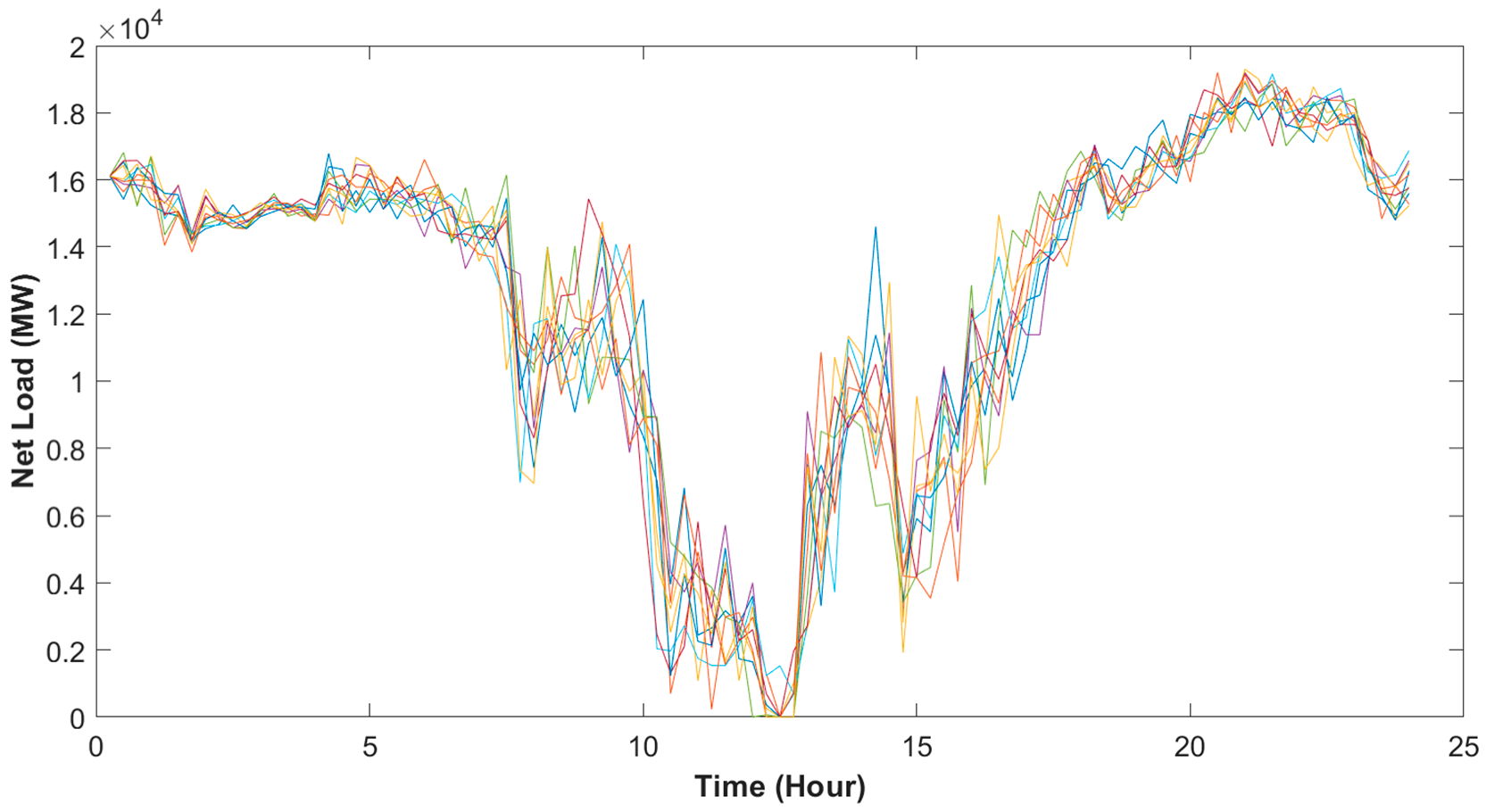
Taiwan has the most challenging unit-scheduling work in autumn, when both wind and solar power outputs operate at almost full capacity, resulting in a net load that is close to zero during the midday period and a high requirement for power ramp-up in the evening. The average unit-scheduling cost in autumn is also the highest among all seasons.

2.

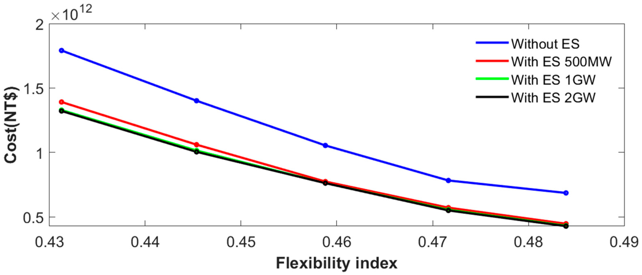
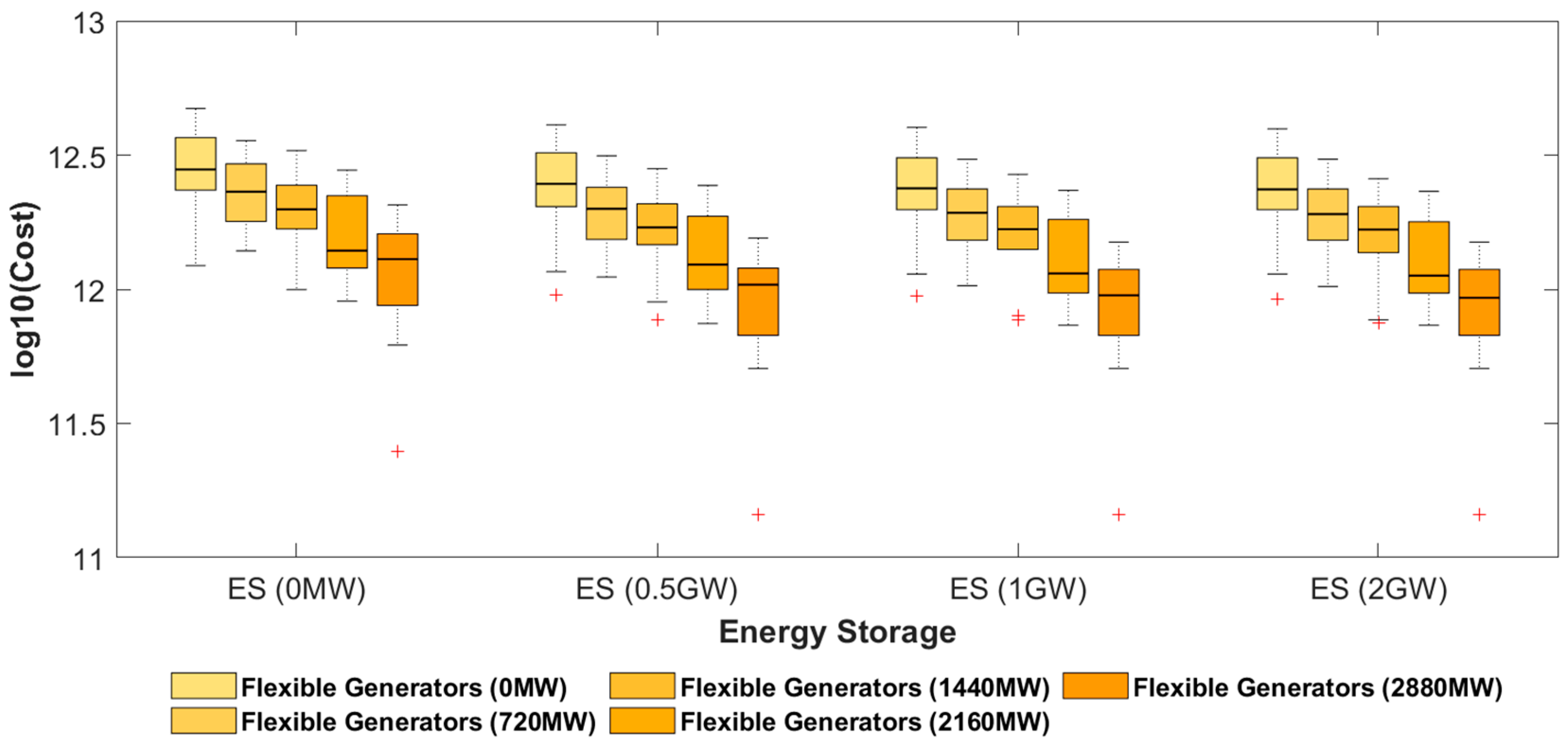
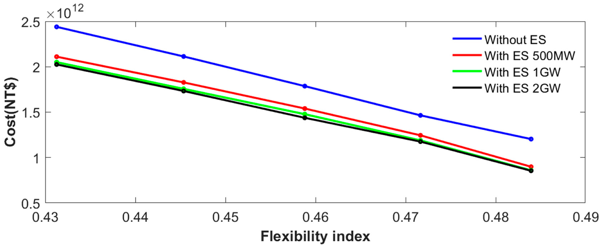
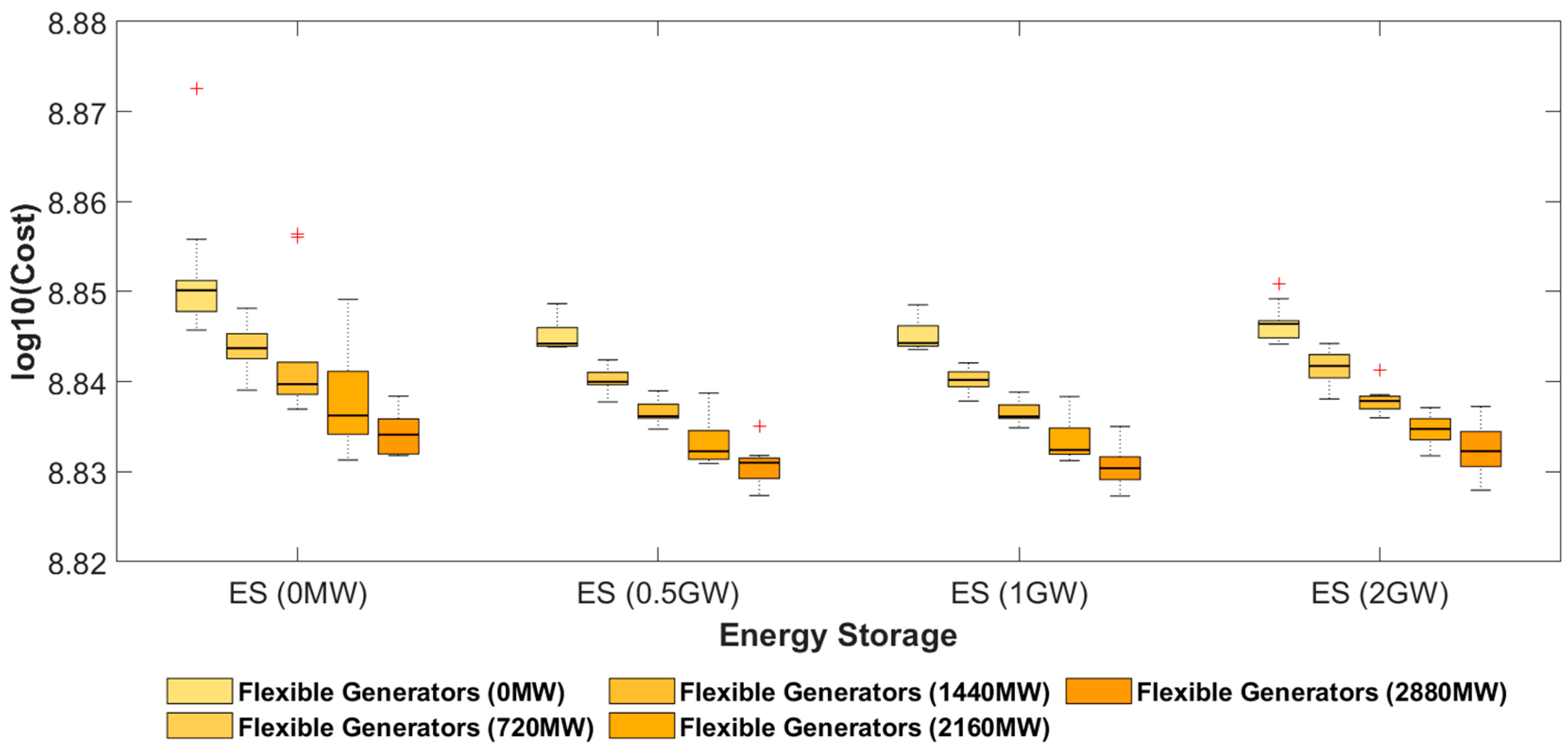
As more flexible units are installed, unit-scheduling costs will be further reduced. However, in terms of economics efficiency, it is not always necessary to increase the capacity of ICE flexible units as much as possible. It is also essential to enhance the forecast accuracy for renewable energy variations and decide an appropriate capacity of flexible units.

3.

For arranging the capacity of energy storages, although a large capacity of storages can reduce unit-scheduling costs in most scenarios, integrating 0.5 GW of energy storage capacity is sufficient for saving most of the dispatching costs and obtaining the most efficient dispatching result. Furthermore, the simulation results also demonstrate that appropriate energy storages effectively provide operating reserves, thus further reducing a shortage of reserve requirements and renewable energy curtailment.

4.

In the future, the integration of large amounts of renewable energy sources will significantly change the current operation strategy on pumped storage units in Taiwan. This study reveals that the period of pumping water into upper reservoir is charged to the peak-load period during the daytime, while the period for generating power is shifted to evening or night.

6. Conclusions

The increase in penetration of renewable generation poses challenges to power system operation and planning. Taiwan is expected to install about 20 GW solar power capacity and 6.5 GW wind power capacity by 2025, in which the power system operator, Taipower, is expected to increase the power system flexibility to cope with a high variability from renewable resources. The study aims to identify the suitable capacity of ICEs and energy storages in the future Taiwan power system in order to maintain a cost-effective grid operation. A flexibility index, quantified with the FAHP method, is utilized to evaluate the equivalent flexibility value of a power system. Furthermore, a stochastic unit scheduling model is formulated for the Taiwan power system, with the consideration of hydro and thermal power units, flexible units (ICEs), energy storage systems, and multi-scenario renewable energy sources. The numerical results demonstrate that Taiwan’s power system will face high variability and intermittency from renewable energy sources in autumn, as both wind and solar energy are operating at full capacity. Unit-scheduling cost is decreased, as a higher capacity of flexible generating units is installed. Lastly, an optimal installed capacity of ICE flexible units (2800 MW) or energy storages (500 MWh) is suggested, according to the generation characteristics of renewable energy sources in each season.

References

1. Mohandes, B.; Moursi, M.S.E.; Hatziargyriou, N.; Khatib, S.E. A Review of Power System Flexibility with High Penetration of Renewables. IEEE Trans. Power Syst. 2019, 34, 3140–3155. [Google Scholar] [CrossRef]
2. Wu, Y.-K.; Tan, W.-S.; Huang, S.-R.; Chiang, Y.-S.; Chiu, C.-P.; Su, C.-L. Impact of generation flexibility on the operating costs of the Taiwan power system under a high penetration of renewable power. IEEE Trans. Ind. Appl. 2020, 56, 2348–2359. [Google Scholar] [CrossRef]
3. Pourahmadi, F.; Heidarabadi, H.; Hosseini, S.H.; Dehghanian, P. Dynamic Uncertainty Set Characterization for Bulk Power Grid Flexibility Assessment. IEEE Syst. J. 2020, 14, 718–728. [Google Scholar] [CrossRef]
4. Ghaljehei, M.; Khorsand, M. Day-Ahead Operational Scheduling with Enhanced Flexible Ramping Product: Design and Analysis. IEEE Trans. Power Syst. 2022, 37, 1842–1856. [Google Scholar] [CrossRef]
5. Khajeh, H.; Laaksonen, H.; Gazafroudi, A.S.; Shafie-khah, M. Towards Flexibility Trading at TSO-DSO-Customer Levels: A Review. Energies 2020, 13, 165. [Google Scholar] [CrossRef] [Green Version]
6. Khoshjahan, M.; Moeini-Aghtaie, M.; Fotuhi-Firuzabad, M.; Dehghanian, P.; Mazaheri, H. Advanced bidding strategy for participation of energy storage systems in joint energy and flexible ramping product market. IET Gener. Transm. Distrib. 2020, 14, 5202–5210. [Google Scholar] [CrossRef]
7. Khoshjahan, M.; Fotuhi-Firuzabad, M.; Moeini-Aghtaie, M.; Dehghanian, P. Enhancing electricity market flexibility by deploying ancillary services for flexible ramping product procurement. Electr. Power Syst. Res. 2021, 191, 106878. [Google Scholar] [CrossRef]
8. Nikoobakht, A.; Aghaei, J.; Shafie-Khah, M.; Catalão, J.P.S. Minimizing Wind Power Curtailment Using a Continuous-Time Risk-Based Model of Generating Units and Bulk Energy Storage. IEEE Trans. Smart Grid 2020, 11, 4833–4846. [Google Scholar] [CrossRef]
9. Li, H.; Lu, Z.; Qiao, Y.; Zhang, B.; Lin, Y. The Flexibility Test System for Studies of Variable Renewable Energy Resources. IEEE Trans. Power Syst. 2021, 36, 1526–1536. [Google Scholar] [CrossRef]
10. Lekvan, A.A.; Habibifar, R.; Moradi, M.; Khoshjahan, M.; Nojavan, S.; Jermsittiparsert, K. Robust optimization of renewable-based multi-energy micro-grid integrated with flexible energy conversion and storage devices. Sustain. Cities Soc. 2021, 64, 102532. [Google Scholar] [CrossRef]
11. Yuan, Y.; Shang, C. Planning of renewable sources and energy storages and retirement of coal plants with unit commitment reserving operational flexibility. In Proceedings of the 2021 IEEE Sustainable Power and Energy Conference (iSPEC), Nanjing, China, 23–25 December 2021; pp. 2282–2286. [Google Scholar]
12. Chen, X.; Lv, J.; McElroy, M.B.; Han, X.; Nielsen, C.P.; Wen, J. Power system capacity expansion under higher penetration of renewables considering flexibility constraints and low carbon policies. IEEE Trans. Power Syst. 2018, 33, 6240–6253. [Google Scholar] [CrossRef]
13. Deason, W. Comparison of 100% renewable energy system scenarios with a focus on flexibility and cost. Renew. Sustain. Energy Rev. 2018, 82, 3168–3178. [Google Scholar] [CrossRef]
14. Internal Combustion Engine. Available online: https://www.wartsila.com/energy/learn-more/technical-comparisons (accessed on 13 June 2022).
15. Tan, W.-S.; Shaaban, M.; Ab Kadir, M.Z.A. Stochastic generation scheduling with variable renewable generation: Methods, applications, and future trends. IET Gener. Transm. Distrib. 2019, 13, 1467–1480. [Google Scholar] [CrossRef] [Green Version]
16. Hu, J.; Li, H. A new clustering approach for scenario reduction in multi-stochastic variable programming. IEEE Trans. Power Syst. 2019, 34, 3813–3825. [Google Scholar] [CrossRef]
17. Du, E.; Zhang, N.; Kang, C.; Xia, Q. Scenario map based stochastic unit commitment. IEEE Trans. Power Syst. 2018, 33, 4694–4705. [Google Scholar] [CrossRef]
18. Elia Grid Data. Available online: https://www.elia.be/en/grid-data (accessed on 13 June 2022).
19. GAMS SCENRED2 Method. Available online: https://www.gams.com/latest/docs/T_SCENRED2.html (accessed on 13 June 2022).
20. Oree, V.; Hassen, S.Z.S. A composite metric for assessing flexibility available in conventional generators of power systems. Appl. Energy 2016, 177, 683–691. [Google Scholar] [CrossRef]
21. Shetaya, A.A.S.; El-Azab, R.; Amin, A.; Abdalla, O.H. Flexibility Measurement of Power System Generation for Real-Time Applications Using Analytical Hierarchy Process. In Proceedings of the 2018 IEEE Green Technologies Conference (GreenTech), Austin, TX, USA, 4–6 April 201; pp. 7–14.
22. Ishizaka, A. Comparison of fuzzy logic, AHP, FAHP and hybrid fuzzy AHP for new supplier selection and its performance analysis. Int. J. Integr. Supply Manag. 2014, 9, 1–22. [Google Scholar] [CrossRef] [Green Version]
Figure 1. The forecasting error of solar power (spring) in the first interval (probability density function (pdf) 01).
Energies 15 05224 g001
Figure 2. The forecasting error of wind power (spring) in the first interval (probability density function (pdf) 01).
Energies 15 05224 g002
Figure 3. Diagram of renewable-energy scenario reduction.
Energies 15 05224 g003
Figure 4. Calculation of flexibility index by FAHP [2].
Energies 15 05224 g004
Figure 5. Scenarios of renewable energy variations in four seasons.
Energies 15 05224 g005
Figure 6. Renewable-energy variation “medium” in 10 sets of net-load scenarios in spring.
Energies 15 05224 g006
Figure 7. Cost comparison of multi-scenario unit scheduling in spring.
Energies 15 05224 g007
Figure 8. Relationship between multi-scenario unit scheduling cost and generation flexibility in spring.
Energies 15 05224 g008
Figure 9. Renewable-energy variation “high” in 10 sets of net-load scenarios in summer.
Energies 15 05224 g009
Figure 10. Cost comparison of multi-scenario unit scheduling in summer.
Energies 15 05224 g010
Figure 11. Relationship between multi-scenario unit-scheduling cost and generation flexibility in summer.
Energies 15 05224 g011
Figure 12. Renewable energy variation “medium” in 10 sets of net-load scenarios in autumn.
Energies 15 05224 g012
Figure 13. Cost comparison of multi-scenario unit scheduling in autumn.
Energies 15 05224 g013
Figure 14. Relationship between multi-scenario unit-scheduling cost and generation flexibility in autumn.
Energies 15 05224 g014
Figure 15. Renewable energy variations “low” in 10 sets of net-load scenarios in the winter.
Energies 15 05224 g015
Figure 16. Cost comparison of multi-scenario unit-scheduling in winter.
Energies 15 05224 g016
Figure 17. Relationship between multi-scenario unit-scheduling cost and generation flexibility in winter.
Energies 15 05224 g017