Continuous Line Loss Calculation Method for Distribution Network Considering Collected Data of Different Densities

Abstract

In order to find the causes of statistical line loss abnormalities and propose better loss reduction strategies, it is necessary to improve the accuracy of theoretical line loss calculations. Since Distributed Generation (DG) access to the distribution network causes variability of power flow in the distribution network within a short period, the error of the traditional line loss calculation method increases. For the line loss calculation of medium-voltage distribution networks containing DGs with high-density collection data, a continuous line loss calculation method for the distribution network was proposed, aiming at improving the accuracy compared with the traditional line loss calculation method. The proposed method makes full use of the high-density collection data on the dispatch side and DG side, distributing the supply power to each load node by power to calculate real-time power flow, thus obtaining a more credible line loss value. The effectiveness and accuracy of the proposed method were verified in the IEEE 17-node distribution system.

1. Introduction

Statistical line loss is the difference between the amount of electricity supplied and the amount of electricity sold, consisting of theoretical line loss and management line loss. Management line loss is the line loss caused by measuring errors, poor management, etc. The theoretical line loss is the actual loss of the power network in the process of transmission and distribution of electric energy. By calculating the theoretical line loss, the composition of the loss in the power network can be clarified, such as the proportion of fixed loss and variable loss, loss at all levels of the power network, loss in each component, transformer loss, and transmission line loss ratio, etc. This facilitates line loss managers to have a comprehensive grasp of the line loss situation, which is conducive to the management of line loss. Theoretical line loss has also been used by power grid companies to study the sources of line loss. In order to find the causes of statistical line loss anomalies and target better loss reduction strategies, improving the accuracy of theoretical line loss calculations is an important task in the work of power companies, improving the lean management of power systems and providing help to further improve the economy of power grids.

At present, the commonly used theoretical line loss calculation methods include the root-mean-square current method, average current method, loss power factor method, forward back generation method, power flow calculation, and equivalent resistance method, etc. [1,2,3,4]. Among them, the root-mean-square current method is simple to calculate, but the accuracy of the method cannot be guaranteed due to the complex structure of the distribution network and imperfect parameters, and the resulting error can reach −23% to 29% [5]. The average current method needs to assume that the power factor and load curve of each load node is the same as the first branch of the network, ignoring the loss of voltage along the line, so there is a certain error in the calculation results. Besides, the power fluctuation also affects the determination of the shape factor [6]. Power flow calculation is prone to the problem of convergence failure caused by inappropriate initial values due to large voltage fluctuations in the distribution network. The structure of medium voltage distribution networks is complex and diverse, which results in difficulties in data collection [7,8]. The equivalent resistance method is widely used in medium- and low-voltage distribution networks due to the small amount of data required and simple calculation. The equivalent resistance method uses the same conditions as the average current method in calculating the equivalent resistance, and thus has the same problems; the loss factor method uses the maximum value of the load curve to calculate the equivalent relationship with the root mean square value, which requires less calculation data, but the loss factor is not easy to calculate, and the calculation accuracy is lower [9,10,11].

In response to the sustainable development policy, DG as a new energy technology is emerging rapidly, gradually occupying a higher and higher proportion in the power grid due to advantages of low cost, environmental protection, location flexibility, etc. When connected to DGs, the structure of the distribution system changes from a radial type to a multi-power type, and the magnitude and direction of tidal currents might change significantly, resulting in changes in the steady-state voltage of the distribution network as well [12]. Reference [13] analyzed the influence of DG on electric power quality, mainly in terms of harmonic voltage levels, and DG may also have a large impact on the original relay protection of the distribution network [14,15,16,17]. The reliability of the system may also be reduced due to the high uncertainty of DG (e.g., photovoltaic cells affected by solar radiation intensity). Reference [18] investigated the optimal load shedding problem when a distribution network containing a DG system undergoes a large disturbance and is in an emergency condition. Reference [19] proposed a DG island operation strategy that can improve the system reliability. With the increasing penetration of new energy, the power balance, power market, and other grid operation uncertainties increase. Therefore, the randomness and volatility of new energy power could cause more complex grid loss mechanisms and loss reduction problems [20]. References [21,22,23] analyzed the impact of DG access capacity and access location on distribution network line losses. The traditional line loss calculation method has some limitations in calculating the line loss for distributed networks with DGs. Reference [24] proposed a new algorithm for loss allocation in distribution systems involving DG units. The algorithm is based on the power injected into the grid lines and considers the active and reactive currents of each line for loss allocation. References [25,26] adopted the equivalent power method to deal with small power sources connected to the distribution network. References [27,28] analyzed the impact of DG access on the distribution network line loss calculation from the perspective of the impact of DG access on the power flow distribution and power quality, respectively, proposing corresponding improved calculation methods. The existing Chinese power industry standard [29] used the equivalent electricity (capacity) method for the theoretical calculation of line loss in distribution networks with small DG access, and to calculate the distribution network line loss in time according to the power flow direction of small power supply. Reference [30] proposed a line loss calculation method based on the load flow calculation for a multi-DGs distribution network, which takes into account the effect of line voltage drop on line losses. However, the load data used in reference [31] are the values after distributing the total load by distribution capacity instead of real-time data, resulting in certain errors.

As stated above, the existing research mainly focuses on the improvement of the algorithm. In most studies, DG is still treated as a general load node in the model. However, with the improvement of distribution network automation, the DG is usually equipped with high-density collection devices. The data collection of DG presents higher-density characteristics such as the dispatching system, including real time information such as voltage, current, active power, and reactive power of each node with DG. However, traditional methods such as the equal resistance method do not make full use of the collected high-density data. Therefore, a continuous calculation method for the line loss calculation method for distribution networks considering collected data of different densities was proposed in this paper, aiming at improving the accuracy of line loss calculation. The total input power of the distribution network was calculated based on the instantaneous value of power of the first branch and DGs. Based on the total input power, the load of each node was proportionally distributed according to the electric quantity information collected by the power meter of each load node. The real-time line loss power was obtained by power flow calculation, and the representative daily total line loss was obtained by summing over time. The effectiveness and accuracy of the proposed method were verified in the IEEE 17-node distribution system.

2. Distribution Network Power Flow Calculation Considering Partial High-Density Collection Data

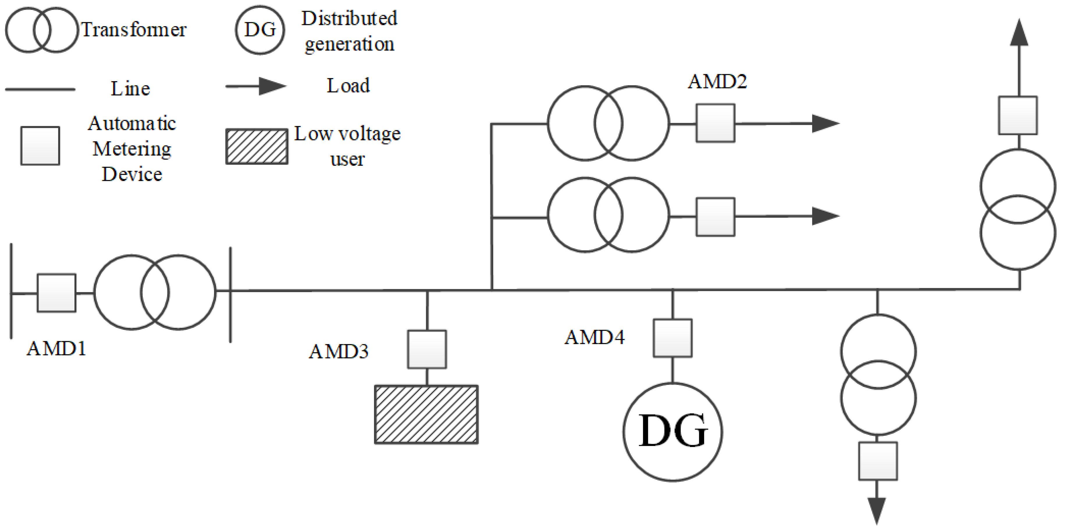
2.1. Medium Voltage Distribution Network Equipped with Automated Collection Equipment

The distribution network is generally a radial structure with scattered data, many points, and less information per point, making it more difficult to collect information than the transmission network. The distribution network data are mainly divided into four categories: active distribution network operation status and related monitoring information, such as network operation topology, DG, and equipment status information; distribution network-related regional weather information affecting DG output, such as light, temperature, wind speed, and other information; and state and marketing information of users in the network, such as electric vehicle operation information, user’s electricity consumption information, etc. With the improvement of the level of information technology, automation, and interaction of smart distribution networks, the data collected at the access end of DG are no longer only the active and reactive power information for a period of time, but present high-density characteristics, i.e., real-time voltage and current data can be collected. If these data can be effectively used in the calculation, the accuracy of the calculation results will be improved.

The power enterprises require that each unit should actively construct and complete the automatic power measuring system platform at the gates to reach “full coverage” of power measuring at all gates, “no shortcomings and no errors” in data return, and meet the functions of statistical calculation of power units at all levels, theoretical calculation of line loss, management of various gateways, management of system parameters, basic data search, system architecture, and topology analysis. The corresponding basic information should be renewed and maintained as soon as possible after the measuring equipment and operation mode of the grid change. Figure 1 shows the schematic diagram of a 10 kV distribution network with DG equipped with automated measuring devices.

As shown in Figure 1, the measuring devices can be classified into the following four types according to their installation locations.

(1)

10 kV distribution network at the transformer connected to the higher-level grid

As shown in AMD1 in the figure, the measuring cycle is usually short, around 1~5 s, to meet the dispatching requirements, and the measuring information includes voltage, current, power, etc. at the first branch of the network.

(2)

Low-voltage side of the transformer in the station area

As shown in AMD2 in Figure 1, the measurement data consist of voltage, current, power, and electricity.

(3)

The connection of low-voltage users to the grid

As shown in AMD3 in Figure 1, the measurement data consist of voltage, current, power, and electricity.

(4)

The connection of DG to the grid

As shown in AMD4 in Figure 1, the measurement data consist of voltage, current, forward and reverse power, and electricity.

For example, the distributed photovoltaic is connected to the electricity consumption collection system, and the data items read include forward total active energy, reverse total active energy, voltage, current, active power, reactive power, and power factor, etc. The electricity consumption collection system works in the following way: the energy meter will freeze the data of the meter at that time at each collection point and store it in the energy meter. The collection terminal will test the smart meters in the station area one by one according to the set time and store the data in the storage unit of the concentrator, and then transmit it to the main station through uplink communication. The more data are collected, the higher the storage capacity and transmission frequency of the concentrator.

The existing technical requirements related to DG collection devices for distribution networks up to 35 kV are as follows:

(a)

DG information collection device uploads full telemetry and telematics data every 5 min (time interval can be matched).

(b)

DG information collection device uploads electricity data once every 15 min (time interval can be assigned).

2.2. Medium Voltage Distribution Network Data Characteristics

Based on the above actual situation, the information of the distribution network is summarized with the following characteristics.

(1)

The data types are diverse. The collected data mainly include electricity consumption, A, B, and C three-phase voltages, and A, B, and C three-line currents as well as active and reactive power, terminal, and equipment information.

(2)

Large data volume. The sampling interval for monitoring terminal voltage, current, and power data is 5–30 min (adjustable in units of 5 min). At present, the sampling interval of the domestic distribution monitoring terminal device is generally 15 min, that is, a node collects 96 points a day. If 10,000 data collection meters have a collection frequency of 15 min/point, one collection can generate 32.61 GB of data, and the data volume will reach 90 TB in a month, which is a very large scale of data [19]. The collection frequency for key users will be higher, such as 5 min/point.

(3)

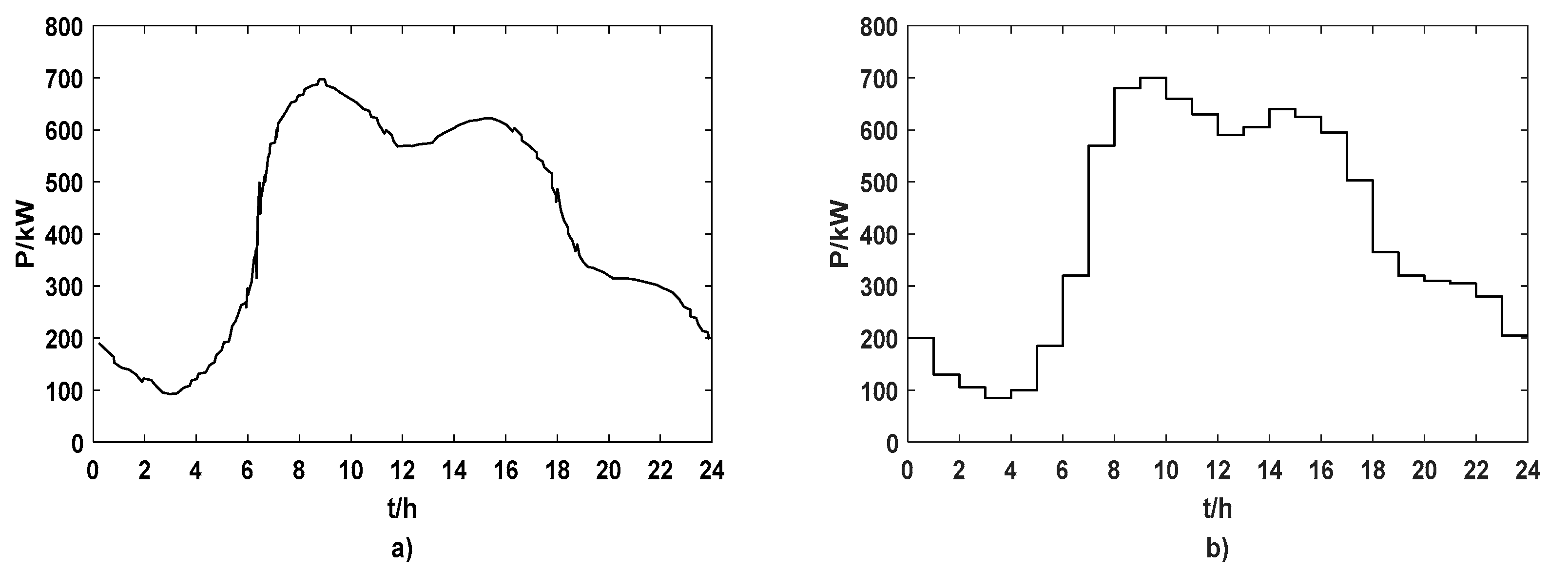
Inconsistent data collection density. The available data can be divided into high-density data and low-density data. 24-point collection means that data are collected once every hour, and the calculated value of this time period is considered to be the average value of this hour; 96-point collection means that data are collected every 15 min, using the average value of those 15 min for calculation. In this paper, the data collected at 96 points and below were considered as low-density data, and those collected at one point per minute were considered as high-density data.

The high-density data are mainly power type, including voltage and current data of fault recording equipment at the first branch of the network, and terminal voltage. The sources of high-density data are the line exit, fault recording, and data collection terminals. In Figure 1, the data collected by AMD1 and AMD4 are high-density data collected once every minute.

The low-density data are mainly the collected power information. AMD2 and AMD3 in Figure 1 collect power data every 15 min. The collected data are low-density data.

Traditional theoretical line loss calculation requires the calculation of multiple time sections, for example, 24-point calculation requires choosing a time section to calculate a theoretical line loss each hour, and considering this time section calculated value as the average value of the hour. This assumption can provide an estimated value of line loss in the case of short time and no big changes in the system state, and the calculation accuracy can meet the engineering needs. However, the volatility of the load in the distribution network is large, and the random volatility of the distributed power supply output leads to the possibility of large changes in the power flow in a short period of time, and the calculation using the average value may cause a large error. Figure 2 shows the daily active load profile, (a) for the actual load and (b) for the calculation load. It can be seen that there is a difference between the calculation load and the actual load, and when the actual load fluctuates widely, the difference increases, and the error of the line loss calculation method using the calculation load increases.

For nodes with DG access, the equivalent resistance method treats DG as a negative power load, which also only uses power information instead of power information, ignoring the fluctuation of DG during the measuring period, and cannot well reflect the change of line loss rate caused by the fluctuation of DG, which also brings error to the results.

In the distribution network with DG access, there are both high-density data and low-density data. If the collected high-density data can be fully utilized, it will help to reduce the error of theoretical line loss calculation caused by load fluctuation.

3. Theoretical Line Loss Calculation of Distribution Network with DG

Although the equivalence resistance method is most commonly used, it has a large error when the load fluctuates drastically. The advantage of the power flow calculation is the high calculation accuracy, and the disadvantage is that it is difficult to use power flow calculation for accurate calculation due to the large amount of data and information that needs to be collected for the distribution network, if the meter is incomplete or the operating parameters are not collected completely, or if the number of components and nodes of the network is too large and the collection and collation of operating data and structural parameters is difficult [19]. This paper used high-density data collection equipment at the first branch of the network and distributed power access points to supplement the low-density data using high-density data to calculate line losses using the power flow of the Newton–Raphson power flow calculation.

3.1. Model of Each Element of Distribution Network with DG

3.1.1. DG Nodes

The measuring information at the DG entry includes voltage, current, forward and reverse power, and electricity. The collection frequency is 1 min/point. The power emitted by the m distributed power outlets at moment t is recorded as:

$$S_h^t=P_h^t+j{Q}_h^t(h=1,2,\cdots ,m)$$

(1)

In the equation, $S_h^t$ is the apparent power emitted by the h-th DG at moment t, $P_h^t$ is the active power emitted by the h-th DG at moment t, and $Q_h^t$ is the reactive power emitted by the h-th DG at moment t.

3.1.2. The First Branch of the Network

The measuring information at the head of the distribution line includes voltage, current, forward and reverse power, and electricity, etc. The collection frequency is 1 min/point. The power flowing through the first node of distribution line at a certain time t is recorded as

$$S_0^t=P_0^t+j{Q}_0^t$$

(2)

In the equation, $S_0^t$ is the power flowing through the first branch of the network at moment t, $P_0^t$ is the active power flowing through the first branch of the network at moment t, and $Q_0^t$ is the reactive power flowing through the first branch of the network at moment t.

3.1.3. The Load Node

The measuring information of the load point includes voltage, current, power, and electricity. The collection frequency is 15 min/point. The active and reactive electric quantity of the n load nodes at the time of (t, t + T) are $W_{pi}$ and $W_{qi}$ (T = 15 min).

3.2. Continuous Calculation Method for Line Loss Calculation Method for Distribution Network Considering Collected Data of Different Densities

The steps of the theoretical line loss continuity algorithm for distribution networks with a mixture of different data densities in this paper are the following:

• Entering known quantities, including branch impedance data, node voltage, and power data, etc. where node data include distribution network head node voltage, distributed power node power and voltage, and load node power within a certain time period.
• Calculating the instantaneous power at the load node.

  (1)

  Calculate the power to be distributed, i.e., the sum of the power at the first branch of the network and the power generated by the DG minus the value of the predicted line loss, as calculated in the following equation.

  $$S_L^t=P_L^t+Q_L^t=S_G^t\ast (1-loss\%)$$

  (3)

  In the equation, $S_L^t$ is the power to be distributed, $P_L^t$ is the active power to be distributed, $Q_L^t$ is the reactive power to be distributed, $S_G^t$ is the sum of the power at the first end of the distribution network and the power generated by distributed power sources, and $loss\%$ is the predicted line loss rate. The predicted line loss rate is taken as the average of the actual line loss rate of the weekday grid. $S_G^t$ is calculated by the following equation.

  $$S_G^t=S_0^t+{\displaystyle \sum S_h^t}=(P_0^t+j{Q}_0^t)+{\displaystyle \sum _{h=1}^{h=m}(P_h^t+j{Q}_h^t)}$$

  (4)

  (2)

  Calculate the instantaneous power at the load node.

  Assuming that the unknown load is distributed proportionally, i.e., the total generator power is distributed proportionally to the load power and counted as the power of the load, the power of each load node at moment t is calculated by the following equation.

  $$P_{li}^t=K_i{P}_L^t$$

  (5)

  In the equation, $P_{li}^t$ is the instantaneous active power absorbed by the i-th load node at moment t, $K_i$ is the power distribution coefficient of the i-th load, and $P_L^t$ is the active power to be distributed in the distribution network at moment t. The calculation of $K_i$ is given in the following equation.

  $$K_i=\frac{W_{pi}}{{\displaystyle \sum _{i=1}^{i=n}{W}_{pi}}}$$

  (6)

  The reactive power of each load node at moment t is calculated by the following equation.

  $$Q_{li}^t=\frac{W_{qi}}{W_{pi}}{P}_{li}^t$$

  (7)

  In the equation, $W_{pi}$ and $W_{qi}$ are the active and reactive electric quantity of the i-th load node at time (t, t + T), respectively, and $Q_{li}^t$ is the instantaneous reactive power absorbed by the i-th load node at time t.

• Forming a nodal conductance matrix based on the known parameters of each node and each branch, the expression of said nodal conductance matrix is:

  $$Y=\left[\begin{array}{ccc}{G}_{11}+j{B}_{11}& \cdots & G_{1n}+j{B}_{1n}\\ ⋮& \ddots & ⋮\\ G_{nn}+j{B}_{nn}& \cdots & G_{nn}+j{B}_{nn}\end{array}\right]$$

  (8)
• Classifying the system node types into three categories: PQ, PV node, and balance node. PQ nodes denote nodes with known active power P and reactive power Q; PV nodes denote nodes with known active power P and node voltage amplitude; and balance nodes denote nodes with known node voltage amplitudes and phase angles. Consider the distribution network head node as the balance node, DG nodes as PQ nodes, and load nodes as PQ nodes. Set the initial values. Write the power equations for PQ nodes and PV nodes.

  $$\{\begin{array}{c}{P}_i=U_i{\displaystyle \sum _{j=1}^n\left(G_{ij}{U}_j\cos {\theta }_j-B_{ij}{U}_j\sin {\theta }_j\right)}\\ Q_i=U_i{\displaystyle \sum _{j=1}^n\left(B_{ij}{U}_j\cos {\theta }_j+G_{ij}{U}_j\sin {\theta }_j\right)}\end{array}$$

  (9)
• The modified equation is as follows.

  $$\{\begin{array}{c}\Delta P_i=P_i-U_i{\displaystyle \sum _{j=1}^n\left(G_{ij}{U}_j\cos {\theta }_j-B_{ij}{U}_j\sin {\theta }_j\right)=0}\\ \Delta Q_i=Q_i-U_i{\displaystyle \sum _{j=1}^n\left(B_{ij}{U}_j\cos {\theta }_j+G_{ij}{U}_j\sin {\theta }_j\right)=0}\end{array}$$

  (10)
• The Jacobian matrix is as follows.

  $$J=\left[\begin{array}{cc}\frac{\partial \Delta P}{\partial {\theta }^T}& \frac{\partial \Delta P}{\partial U^T}\\ \frac{\partial \Delta Q}{\partial {\theta }^T}& \frac{\partial \Delta Q}{\partial U^T}\end{array}\right]$$

  (11)
• Solving the correction equation to obtain the node voltage correction.
• Correcting the voltage at each node.
• Determining whether the convergence condition is satisfied; if so, end the loop; if not, return to step 4.
• Calculating power flow is every minute to obtain real-time line power loss.
• Summing over time to find the total loss of a representative time period or representative day.

4. Case Study

The proposed method in this section was verified on an IEEE 17 node system as shown in Figure 3. The algorithm was written on the MATLAB R2017b platform and run on a PC with CPU model i5-4440, 3.10 GHz, and 6 GB of RAM.

Currently, common smart meters collect 96 points of data, which means that data are collected 96 times a day, once every 15 min. By applying new concentrators to communicate with meters at a high interaction rate of more than a hundred meters per minute on average, real-time active reporting of minute-level electricity consumption data is realized in some places, and these new concentrators are generally applied at the distributed power supply side. So, in this paper, it was assumed that the measuring cycle of the equipment on the power side of the distribution network was 1 min and the measuring cycle of the equipment on the load side was 15 min.

The voltage level of the selected system was 23 kV, with 17 nodes and 16 branches. Among them, Bus 1 is the distribution network head node, Bus 2–17 is the load node, the total active load is 13.88 MW, and the total reactive load is 5.64 MVar. All the network parameters are known, and the distribution network head dispatch data and the load node’s electric quantity in 15 min are known.

Figure 4 shows the single-day output curve of a photovoltaic power plant under four different weather types: sunny, cloudy, windy, rain, and snow. It can be seen that the weather had a significant impact on the fluctuation level of photovoltaic output. Before 5:00 a.m. and after 8:00 p.m. are the night hours when there is no sunlight, so photovoltaic output was zero. The photovoltaic output was stable when it is sunny. After sunrise, as the light intensity increased, the photovoltaic output curve rose, peaking at 2:00 p.m. when the sunlight was strongest, and then decreasing. Photovoltaic output fluctuated significantly during cloudy and windy days because high winds can change the position of clouds. The clouds moved rapidly, and when the clouds moved above the photovoltaic, the photovoltaic output became smaller, and when the clouds moved away, the photovoltaic output increased. Sometimes the fluctuation amount could exceed 50% of the installed capacity in a short period of time when it was cloudy or windy. In rainy and snowy weather, the overall photovoltaic output level was lower due to low sunlight intensity, and the fluctuation of output was smaller than when it is cloudy and windy.

In this system, Bus 3 was connected to No.1 distributed photovoltaic (treated as PQ node), and Bus 5 was connected to No.2 distributed photovoltaic (treated as PQ node). The installed capacity of both photovoltaics was 5 MW. The one-hour photovoltaic power generation curves for these scenarios were simulated according to the fluctuations during the 11:00–12:00 time period in Figure 3, with a fluctuation time scale of 1 min, as shown in Figure 5.

In Figure 5, the typical scenario 1 is the photovoltaic output curve on a sunny day, and the photovoltaic output curve is smooth on a sunny day. Typical scenario 2 is the photovoltaic output curve in cloudy weather. Typical scenario 3 is the photovoltaic output curve on an windy day. Typical scenario 4 is the photovoltaic output curve in rainy and snowy weather. The Figure 5 indicates that the photovoltaic output is smooth in sunny weather, while fluctuating greatly in windy and cloudy weather. In rainy and snowy weather, the overall photovoltaic output level is lower than that in cloudy or windy weather as well as the output fluctuation.

Bus 14 was selected to change the active power output of its connected load feeder within 1 h. The original active power was 0.4 MW, and now it was made to fluctuate in the range of 0.3–0.45 MW, and the time scale of fluctuation was set to 1 min. The load fluctuation is shown in Figure 6.

The traditional equivalent resistance method was used to calculate one hour line loss rate for this system. The Newton–Raphson method was used to calculate the power flow for this system, where node 1 was taken as the balance node and the rest of the nodes were used for power flow calculation as PQ nodes. After four iterations, the system achieved the convergence accuracy requirement. The line loss rate of the representative time period was calculated by the proposed method in this paper, and the results of the three methods were compared with the actual values, as shown in

Table 1. Comparison of three theoretical line loss calculation methods.

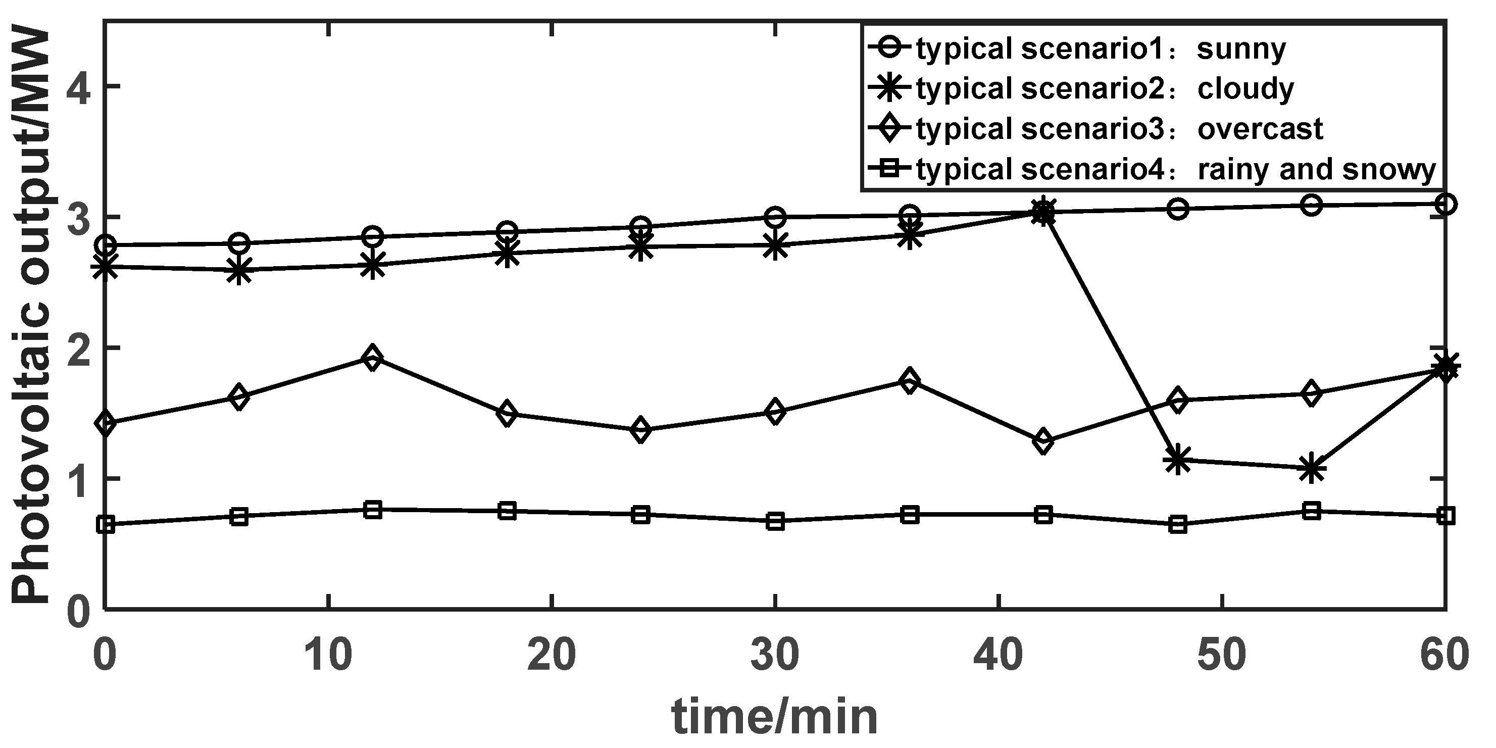
Typical Scenario	Corresponding Weather	Line Loss Rate of Traditional Equivalent Resistance Method	Line Loss Rate of Power Flow Calculation	Line Loss Rate of the Method in This Paper	Actual Line Loss Rate
Scenario 1	sunny	4.78%	4.42%	4.66%	4.72%
Scenario 2	cloudy	5.17%	5.43%	5.73%	5.77%
Scenario 3	windy	6.24%	4.79%	5.05%	5.12%
Scenario 4	rainy and snowy	4.51%	6.00%	6.33%	6.40%

.

The error comparison between each method and the true value is shown in

Table 2. Relative error of three theoretical line loss calculation methods.

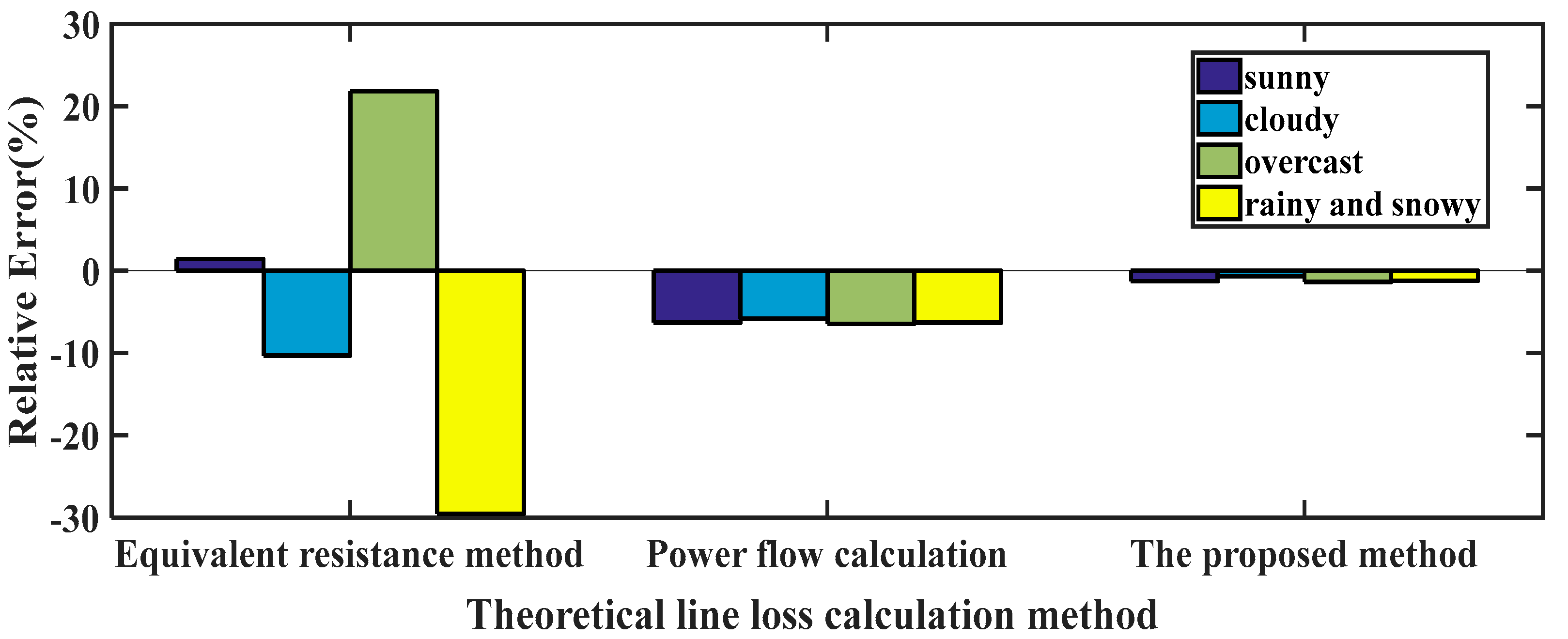
Typical Scenario	Relative Error of Traditional Equivalent Resistance Method	Relative Error of Power Flow Calculation	Relative Error of Method in This Paper
Scenario 1	1.42%	−6.30%	−1.29%
Scenario 2	−10.32%	−5.84%	−0.69%
Scenario 3	21.82%	−6.45%	−1.36%
Scenario 4	−29.56%	−6.32%	−1.21%

.

The data from Table 2 are represented in the form of a bar chart, as shown in Figure 7.

We set the power of all load nodes in the system to fluctuate, with a fluctuation range of 80–120%. The results are shown in the

Table 3. Relative error of three theoretical line loss calculation methods (power fluctuates at all load nodes).

Typical Scenario	Relative Error of Traditional Equivalent Resistance Method	Relative Error of Power Flow Calculation	Relative Error of Method in This Paper
Scenario 1	14.10%	−3.85%	−0.64%
Scenario 2	−4.82%	−3.55%	−0.38%
Scenario 3	−8.84%	−5.80%	−1.45%
Scenario 4	−9.82%	−1.83%	−0.68%

.

We reduced the power of all load nodes by 20%, and the calculation results are shown in

Table 4. Relative error of three theoretical line loss calculation methods (20% reduction in load node power).

Typical Scenario	Relative Error of Traditional Equivalent Resistance Method	Relative Error of Power Flow Calculation	Relative Error of Method in This Paper
Scenario 1	28.09%	−4.26%	−0.43%
Scenario 2	−7.60%	−4.48%	−0.78%
Scenario 3	33.65%	−5.21%	−1.18%
Scenario 4	−10.30%	−3.72%	−1.01%

. We increased the power of all load nodes by 20%, and the calculation results are shown in

Table 5. Relative error of three theoretical line loss calculation methods (20% increase in load node power).

Typical Scenario	Relative Error of Traditional Equivalent Resistance Method	Relative Error of Power Flow Calculation	Relative Error of Method in This Paper
Scenario 1	16.80%	−3.85%	−1.18%
Scenario 2	−13.20%	−2.71%	−0.59%
Scenario 3	10.56%	−3.38%	−0.97%
Scenario 4	−11.76%	−2.02%	−0.11%

.

By comparing the results of the three calculation methods, it can be seen that the traditional equivalent resistance method had the largest error of up to 20% or more in the four typical scenarios. The error in the line loss results is caused by the fact that the equivalence resistance method does not take into account the power fluctuations of DG and loads within a short period of time in the calculation.

The error of the power flow calculation was smaller, at about 6%, and the error value was relatively stable. This is because power flow calculation takes into account the volatility of the DG, but does not take into account the fluctuations of the load within a short period of time. Therefore, the accuracy of power flow calculation is high when the actual load does not fluctuate much in a short period of time.

The results show that the relative error of the proposed method in this paper was around 1%, indicating the accuracy is highest among the three methods. This is because the proposed method makes full use of high density data of DG compared with the equivalent resistance method and power flow calculation.

When multiple DGs are connected to the distribution network, the proposed method, the number of DGs, and the operation mode could not be restricted in the proposed method. In other words, the target distribution network can have an unlimited number of DGs, which can supply power to the grid or absorb power from the grid. When a distributed power source generates electricity, the power it generates is first supplied to the local load for consumption, and the remaining is then sent to the distribution network for distribution to the rest of the load. The proposed method in this paper has generality and can be applied in the actual distribution network.

5. Conclusions

This paper proposed a continuous calculation method for the line loss calculation method for distribution networks considering collected data of different densities. Based on high-density data collection, the real-time output power of each load in the distribution network was obtained by power flow calculation. The proposed method makes full use of collection information of DG and dispatch system, achieving a higher accuracy of line loss calculation as compared with traditional methods.

The results of the example in the IEEE17-node distribution network system demonstrated the accuracy of the method. The simulation results also showed that the method is applicable to line loss calculation in a variety of scenarios and has the potential to be applied in practical distribution networks, providing a basis for line loss analysis and management of distribution network systems with DGs.

References

- Yang, L.X.; Liu, H.; Zhang, H.Y.; Lou, B. Improved shape coefficient method for low voltage grid line loss calculation. Power Demand Side Manag. 2009, 11, 29–32. [Google Scholar]
- Zhang, K.K.; Yang, X.Y.; Bu, C.R.; Ru, W.; Liu, C.J.; Yang, Y.; Chen, Y. Theoretical line loss analysis and loss reduction measures of distribution network based on load measurement. Chin. J. Electr. Eng. 2013, 33, 92–97. [Google Scholar]
- Zhuoqiong, L.; Junchao, Z. Analysis of the factors influencing the loss of medium voltage lines in distribution networks based on mutual information and countermeasure theory. Smart Power 2017, 45, 75–79. [Google Scholar]
- Wang, E.; Cao, M.; Zhang, R.X.; Yang, L.C.; Tang, B.; Lian, X.; Li, B. Research on optimal line loss apportionment method based on spectral mass center migration. Smart Power 2019, 47, 114–120. [Google Scholar]
- Jun, S. A Power Power Flow Calculation for Theoretical Line Loss Calculation. Master’s Thesis, Dalian University of Technology, Dalian, China, 2004. [Google Scholar]
- Chen, D.Z.; Guo, Z.Z. Theoretical line loss calculation for distribution networks based on load acquisition and matching power flow calculation. Grid Technol. 2005, 29, 80–84. [Google Scholar]
- Liu, D.; Chen, Y.P.; Shen, G.; Fan, Y.P. Impact of load randomness on line loss calculation and distribution network reconfiguration. Power Syst. Autom. 2006, 9, 25–28+55. [Google Scholar]
- Fu, Z.W.; Liu, H.J. Line loss calculation of power system considering the influence of load curve and generation output curve. Guangxi Electr. Power 2004, 4, 1–3. [Google Scholar]
- Zhu, Z.Z.; Ye, F.J. An improved algorithm for theoretical line loss calculation of low-voltage distribution networks. Electr. Meas. Instrum. 2012, 49, 6–10. [Google Scholar]
- Shu, Q.Q.; Xiao, J.H.; Ren, W.M.; Yang, L.; Chen, L.K. Research on distribution network line loss analysis methods in power systems. Autom. Instrum. 2018, 3, 28–31. [Google Scholar]
- Zhang, Q.X.; Chang, G. Analysis of distribution network line loss calculation methods and their applicability. China Rural. Water Conserv. Hydropower 2015, 5, 180–184. [Google Scholar]
- Scott, N.C.; Atkinson, D.J.; Morrell, J.E. Uses of load control to regulate voltage on distribution network swish embedded generation. IEEE Trans. Power Syst. 2002, 17, 510–515. [Google Scholar] [CrossRef]
- Kojovic, L. Impact of DG on voltage regulation. In Proceedings of the Power Engineering Society Summer Meeting, Chicago, IL, USA, 21–25 July 2002; pp. 160–165. [Google Scholar]
- Dolezal, J.; Santarius, P.; Tlusty, J. The Effect of dispread generation on power quality in distribution system. In Proceedings of the CIGRE/IEEE PES International Symposium, Montreal, QC, Canada, 8–10 October 2003; pp. 204–207. [Google Scholar]
- Dugan, R.C. Operation conflicts for distributed generation system. In Proceedings of the Rural Electric Power Conference, Little Rock, AR, USA, 29 April–1 May 2001; pp. 401–405. [Google Scholar]
- Zeineldin, H.H.; Sharaf, H.M.; Ibrahim, D.K.; El-Zahab, E.E.-D.A. Optimal Protection Coordination for Meshed Distribution Systems With DG Using Dual Setting Directional Over-Current Relays. IEEE Trans. Smart Grid 2014, 6, 115–123. [Google Scholar] [CrossRef]
- Sookrod, P.; Wirasanti, P. Overcurrent relay coordination tool for radial distribution systems with distributed generation. In Proceedings of the 2018 5th International Conference on Electrical and Electronic Engineering (ICEEE), Istanbul, Turkey, 3–5 May 2018; pp. 13–17. [Google Scholar]
- Xu, D.; Girgis, A. Optimal load shedding strategy in power systems with distributed generation. In Proceedings of the IEEE Power Engineering Society Transmission and Distribution Conference, Columbus, OH, USA, 28 January–1 February 2001; pp. 788–793. [Google Scholar]
- Hegazy, Y.G. Intention islanding of distributed generation for reliability enhancement. In Proceedings of the CICGE/IEEE PES International Symposium, Montreal, QC, Canada, 8–10 October 2003; pp. 208–213. [Google Scholar]
- Liu, Y.; Wang, C.Y.; Xia, D.M. Analysis of the impact of grid faults on grid frequency due to large area wind power LVRT and measures. Power Grid Technol. 2021, 45, 3505–3514. [Google Scholar]
- Chiradeja, P.; Ngaopitakkul, A. The impacts of electrical power losses due to distributed generation integration to distribution system. In Proceedings of the International Conference on Electrical Machines and Systems (ICEMS), Busan, Korea, 26–29 October 2013; pp. 1330–1333. [Google Scholar] [CrossRef]
- Ymeri, A.; Dervishi, L.; Qorolli, A. Impacts of Distributed Generation in Energy Losses and voltage drop in 10 kV line in the Distribution System. In Proceedings of the 2014 IEEE International Energy Conference (ENERGYCON), Dubrovnik, Croatia, 13–16 May 2014; pp. 1315–1319. [Google Scholar] [CrossRef]
- Chiradeja, P.; Ngaopitakkul, A. The impact of capacity and location of multidistributed generator integrated in the distribution system on electrical line losses, reliability, and interruption cost. Environ. Prog. Sustain. Energy 2015, 34, 1763–1773. [Google Scholar] [CrossRef]
- Khosravi, M.; Monsef, H.; Aliabadi, H.M. Loss allocation in distribution network including distributed energy resources (DERs). Int. Trans. Electr. Energ. Syst. 2018, 28, e2548. [Google Scholar] [CrossRef]
- Han, S.; Gao, X.N.; Qiu, G.Y.; Gao, H.; Zhao, W.H.; Song, H. Estimation method of distribution network line loss considering distributed power sources. J. Power Sci. Technol. 2009, 24, 76–82. [Google Scholar]
- Shi, L.Z.; Luo, Y.F.; Liu, W.; Chen, G.B. A solution to the problem of calculating small and medium power sources for distribution network line loss theory--equivalent capacity method. Cent. China Electr. Power 1997, 5, 11–13. [Google Scholar]
- Wang, H.K.; Wang, S.X.; Pan, Z.X.; Wang, J.M. Optimized scheduling method for flexibility enhancement of distribution networks containing high penetration distributed power sources. Power Syst. Autom. 2018, 42, 86–93. [Google Scholar]
- Luo, T.Y. Calculation and Optimization of Cross-Regional Large Grid Losses. Master’s Thesis, Shenzhen University, Shenzhen, China, 2019. [Google Scholar]
- Fu, X.Q. Optimal Allocation of DG Considering Line Loss and Power Quality of Distribution Network. Master’s Thesis, South China University of Technology, Guangzhou, China, 2015. [Google Scholar]
- He, X.H. A Theoretical Line Loss Calculation Method for Distribution Networks with Distributed Power Sources. Master’s Thesis, Hunan University, Changsha, China, 2009. [Google Scholar]
- Zu, Y. Power Quality Analysis Method Based on Electricity Consumption Information Collection Data. Master’s Thesis, Xi’an University of Technology, Xi’an, China, 2020. [Google Scholar]