Sub-Optimal Stabilizers of the Pendubot Using Various State Space Representations

Abstract

This paper considers the issue of linear-quadratic regulator (LQR) design for nonlinear systems with the use of smooth state and input transformations. The proposed design methodology is considered in the stabilisation task of the Pendubot, which is based on the concept of feedback equivalent control systems. It turns out that it is possible to find a controller that ensures comparable dynamics of the closed-loop system in the vicinity of the set point regardless of the state-space representation adopted. In addition, the synthesis of suboptimal controllers according to the LQR strategy ensuring equal dynamics at the equilibrium point is presented. The properties of the studied controllers were investigated in a simulation environment and using experimental tests. The detailed forms of transformations and linear approximations given can be regarded as ready-made procedures that can be applied to stabilise similar mechanical systems in robotics.

1. Introduction

The problem of designing optimal feedback to stabilize dynamic systems can be regarded as one of the fundamental issues of control theory. In particular, for a class of time-invariant linear (LTI) systems, this problem is already well recognized. One of the essential control design approaches to stabilize these systems is based on the minimization of an energetic-like quadratic performance index involving the state trajectory and input, which leads to the linear-quadratic regulator commonly known as LQR. This approach has a long and rich history, dating back to the early work of Kalman [1], who discussed the problem of optimal feedback, providing the design equations for LQR.

Feedback design becomes more challenging in the case of nonlinear systems, for which the search for an optimal controller can be a complex problem that cannot be solved by analytical methods. One important tool in control design is to resort to a linear approximation of the nonlinear dynamics around the equilibrium point under condition that the corresponding linear model is controllable in the sense of Kalman. A known limitation of this approach is the local nature of the solution, which imposes restrictions on the set of admissible initial conditions. In such circumstances, the LQR approach is capable of providing only suboptimal results. Despite that, LQR still constitutes an essential method for dealing with the control of nonlinear systems. In particular, it is able to guarantee a local exponential convergence, that provides robustness to some class of uncertainties [2]. For this reason, the method is of great importance in robotics, where the predominant group of mechanical systems exhibit strongly nonlinear properties. Recently, one can find publications that discuss applications of the LQR method, often in the context of complex hybrid techniques for the control of manipulators with rigid or compliant joints [3,4,5]. In particular, LQR-based control solutions have been proposed for a class of underactuated systems [6,7,8,9]. In some cases LQR approach is used as a tuning method for strictly nonlinear controllers, see for instance [10]. Modifications of LQR for nonlinear systems have been considered, such as the state-dependent Riccati equation (SDRE) approach [11] and its various implementations [12,13,14]. In addition, techniques inspired by differential dynamic programming [15,16] lead to iterative LQR (iLQR) [17,18], for which the dynamics are linearized in a sequence and the cost function about a given nominal trajectory is computed to find an LQR control policy. Based on a similar idea, the LQR-equivalent of Kalman smoothing has been reported in [18].

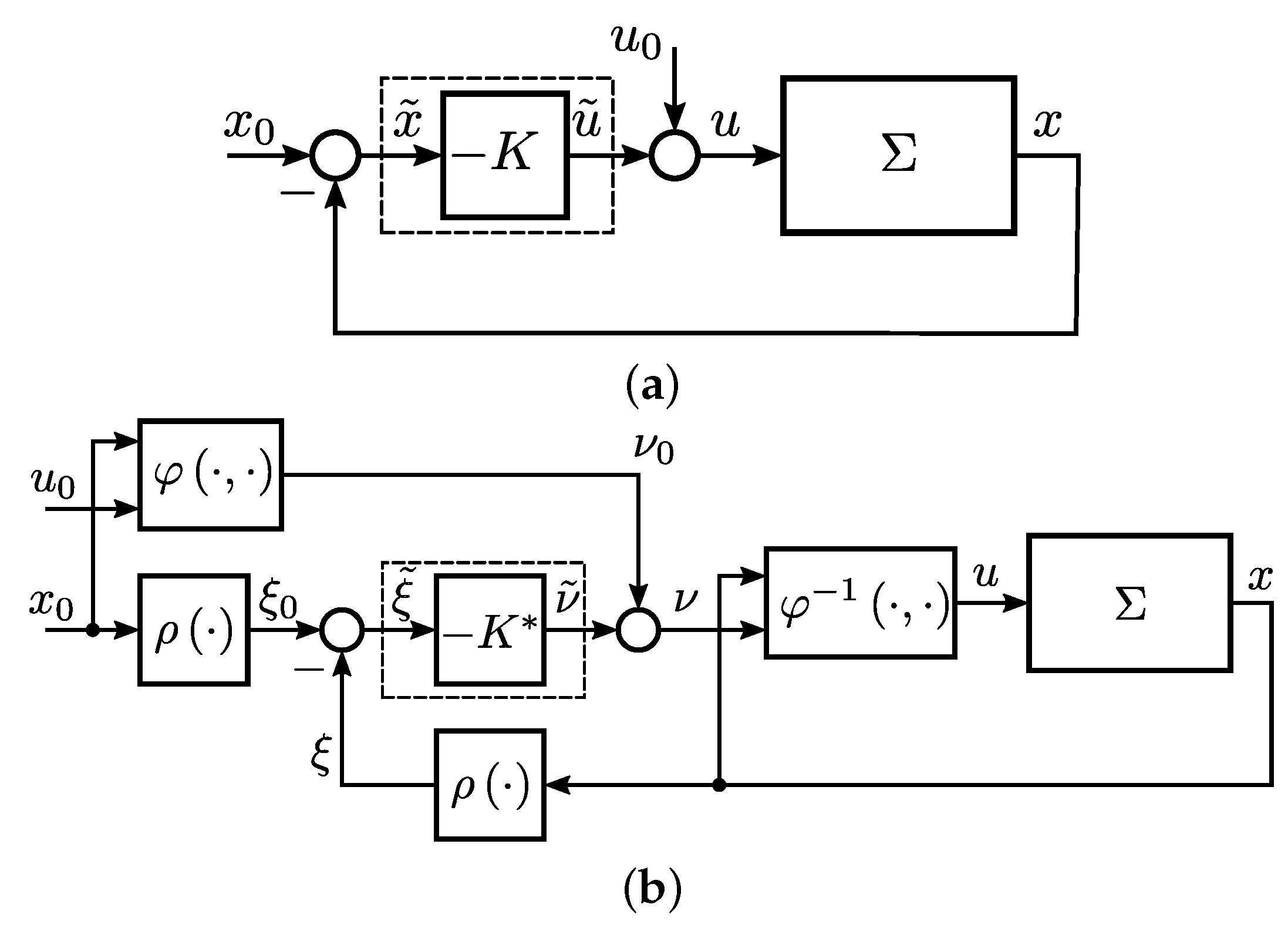
In this paper, we refer to nonlinear control theory and use the concept of feedback-equivalent control systems [19] in order to improve the performance of the LQR design by extending the set of feasible initial conditions that define the so-called basin of attraction. The considered methodology is to use a linear state feedback designed for the linear approximation of a feedback-equivalent control system, and determine a stabilizer taking advantage of state and input maps. A key ingredient is the transformation of the original dynamics to a form that exhibits better characteristics for synthesizing a linear regulator. In particular case, the equivalent dynamics can be even linear [20], which can considerably improve the controller performance in a given subset of the state space at which linearization is possible. In this context, it may be important to estimate the area of convergence. An important tool here is Lapunov analysis [21,22] and the use of nonlinear numerical and analytical methods such as the sum of squares (SOS) [23,24], which allow for a less restrictive approximation.

From the point of view of control objectives, the design of the LQR should take into account the quality index determined for the original system, i.e., taking into account the state of this system and the energy expenditure associated with the actual input. Therefore, in the case of the feedback design based on the transformed system, the question of the LQR tuning criterion seems to be important [25,26]. This issue is analyzed in this work. We show here a solution to determine the gains that ensure comparable dynamics of the closed-loop system in the vicinity of the set point regardless of the state and input representation adopted. In addition, we provide an equivalent quadratic form that describes the optimization criterion with respect to the transformed dynamics.

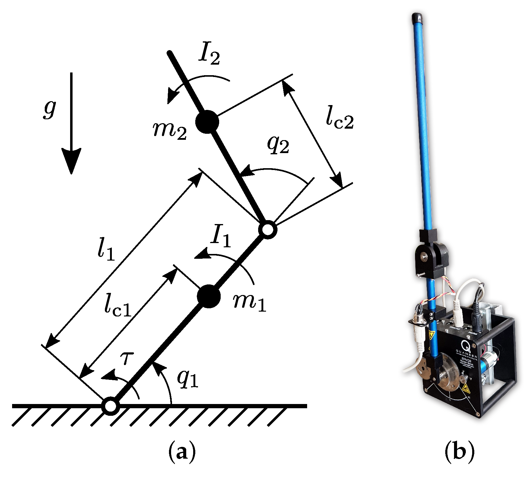
In this paper, the control methodology considered is used to design a Pendubot stabilizer. This system, along with Acrobot and the inverted pendulum, can be considered as a benchmark underactuated system in robotics [27,28,29]. We deal with the stabilization of the Pendubot at up-right position without taking into account the swing-up problem. Instead, the problem investigated here is focused on the design of a smooth state feedback at a neighborhood of the desired point taking advantage of the concept of feedback equivalent control systems. Although, the linear approximation of the Pendubot at an equilibrium point is controllable, the system is not fully linearizable using state and input transformations. Furthermore, as discussed precisely in [30], there are also significant obstructions in the application of the partial linearization approach, while this method cannot be directly employed for stabilization due to the presence of singular points [31].

To investigate the effect of the state-space representation on the characteristics of the closed-loop system, the original Langrange dynamics of the Pendubot is transformed into two alternative forms. These forms take advantage of the so-called quasi-velocities, which in analytical mechanics are understood as linear combinations of generalized velocities with coefficients that are functions of the generalized coordinates [32,33]. In the first form, the inertial normalized quasi-velocities (NQV) proposed by Jain and Rodriguez in [34,35] which comes from the factorization of the inertia matrix, are used. In particular, the transformations proposed for the Pendubot to design a swing-up controller [36], in this paper are used for the stabilization task. It turns out that quasi-velocities along with the nonlinear transformation of the coordinates can be used to represent the Pendubot dynamics in the so-called normal form [37]. Such a form, considered among others in classification problems, highlights in an organized way the essential features of a nonlinear dynamic system [30].

The new contributions to this paper include the following:

• Comparison of Pendubot mathematical models using different representations, including application of quasi-velocities;
• Synthesis of sub-optimal controllers according to the LQR strategy ensuring equal dynamics at the equilibrium point;
• Simulation comparison of the controllers and determination of the convergence area under constrained input conditions;
• Conducting experimental tests and obtaining results illustrating properties of controllers.

It is noteworthy that another purpose of the work is to adapt the control algorithm to the real system and to show reproducible results. To the authors’ knowledge, in many publications on stabilization of Acrobot and Pendubot-type mechanical structures, real-based models are not explicitly investigated and primarily the basic models proposed in Spong’s works are recalled. Often, other works do not contain sufficient information about the model and controller parameters, or are tested for a non-physical system. Our aim is to dispel these doubts through experimental verification and research on stability or the area of convergence of the algorithm. Therefore, the experiments have been carried out for a system that can be built from components of a commercially available system. For this reason, the results shown in the paper can be treated as a basis for future comparisons.

The paper is organized as follows. In Section 2 the nominal dynamics of the Pendubot are recalled. Section 3 deals with feedback-equivalent control systems and describes two equivalent models of the Pendubot taking into account the inertial normalized quasi-velocities (NQV) and transformation to the normal form (NF). In Section 4, the design of the controller based on the LQR approach and its stability issues are discussed. In Section 5 simulation and experimental results are presented. Section 6 discusses the results obtained, and Section 7 ends with general conclusions and plans for future research.

2. Model

Let us consider the mechanical system presented in Figure 1 with the state chosen as $x={\left[q^T{\omega }^T\right]}^T\in S^1\times S^1\times {\mathbb{R}}^2$, where $q={\left[q_1{q}_2\right]}^T$ stands for the system configuration and $\omega ={\left[{\omega }_1{\omega }_2\right]}^T$ denote velocities, while $q_i$ and ${\omega }_i$ describe the angular displacement and angular velocity of the $i\mathrm{th}$ link ($i=1,2$), respectively. The system input $u=\tau \in {\mathbb{R}}^{}$ corresponds to the torque exerted on the first joint. In the state-space representation, the dynamics of the Pendubot can be described as follows

$$\dot{x}=\left[\begin{array}{c}\omega \\ D^{-1}\left(q\right)\left(-C\left(q,\dot{q}\right)\dot{q}-G\left(q\right)+bu\right)\end{array}\right],$$

(1)

where

$$D\left(q\right)=\left[\begin{array}{cc}{a}_1+a_2+2a_3\cos q_2& a_2+a_3\cos q_2\\ a_2+a_3\cos q_2& a_2\end{array}\right]$$

(2)

is the inertia matrix,

$$C(q,\dot{q})=\left[\begin{array}{cc}-a_3\sin q_2{\dot{q}}_2& -a_3\sin q_2({\dot{q}}_1+{\dot{q}}_2)\\ a_3\sin q_2{\dot{q}}_1& 0\end{array}\right]$$

(3)

is the centrifugal and Coriolis matrix,

$$G\left(q\right)=\left[\begin{array}{c}{a}_5\cos (q_1+q_2)+a_4\cos q_1\\ a_5\cos (q_1+q_2),\end{array}\right]$$

(4)

describes gravity torques and $b={\left[10\right]}^T$ is the input matrix. The constant coefficients $a_j$, $j=1,2,\cdots ,a_5$, satisfy: $a_1=m_1{l}_{\mathrm{c}1}^2+m_2{l}_1^2+I_1$, $a_2=m_2{l}_{\mathrm{c}2}^2+I_2$, $a_3=m_2{l}_1{l}_{\mathrm{c}2}$, $a_4=g\left(m_1{l}_{\mathrm{c}1}+m_2{l}_1\right)$ and $a_5=g{m}_2{l}_{\mathrm{c}2}$.

3. Equivalent Models of the Pendubot in Quasi-Velocities

3.1. Feedback Equivalent Control Systems

In this paper, we deal with feedback-equivalent control systems [19]. To describe the concept formally, let us introduce the following smooth dynamic systems.

$$\begin{array}{cc}\hfill \Sigma :\dot{x}& =f\left(x,u\right),\hfill \end{array}$$

(5)

$$\begin{array}{cc}\hfill {\Sigma }^{*}:\dot{\xi }& =f^{*}\left(\xi ,\nu \right),\hfill \end{array}$$

(6)

where $x\in X\subseteq {\mathbb{R}}^n$, $\xi \in \mathsf{\Xi }\subseteq {\mathbb{R}}^n$ denote states, while $u,\nu \in {\mathbb{R}}^m$ are inputs and $f:X\times {\mathbb{R}}^m\to {\mathbb{R}}^n$, $f^{*}:\mathsf{\Xi }\times {\mathbb{R}}^m\to {\mathbb{R}}^n$ are smooth state functions. It is assumed that these systems are equivalent under the change of states,

$$\xi =\rho \left(x\right)$$

(7)

and inputs,

$$\nu =\phi \left(x,u\right),$$

(8)

with $\rho :X\to \mathsf{\Xi }$ and $\phi :X\times {\mathbb{R}}^m\to {\mathbb{R}}^m$ being local diffeomorphisms. To facilitate further investigations, the inverse of the input map (8) is also introduced as:

$$u={\phi }^{-1}\left(x,\nu \right).$$

(9)

From there, system $\Sigma$ will be considered the nominal dynamics of the Pendubot represented by (1), while system ${\Sigma }^{*}$ will be regarded as a transformed version of this dynamic model. In the following subsections, alternative representations of this model will be taken into account. The first representation is based on the decomposition of the mass matrix, while the second comes from the transformation to the so-called normal, which is characterized by a cascade-like structure.

3.2. Transformation Based on Inertial Normalized Quasi-Velocities (NQV)

The concept of inertial normalized quasi-velocities (NQV) proposed by Jain and Rodriguez in the work [34,35] comes from the factorization of the inertia matrix, which is positive definite, non-singular and symmetric. For this purpose, Cholesky factorization can be taken into account. Applying this method with respect to matrix (2) one can write that:

$$D\left(q\right):=L\left(q\right)L^T\left(q\right),$$

(10)

where

$$L\left(q\right)=\left[\begin{array}{cc}\sqrt{d_2\left(q_2\right)}& \sqrt{a_2}(1+a_{32}\cos q_2)\\ 0& \sqrt{a_2},\end{array}\right]$$

(11)

with $a_{32}=\frac{a_3}{a_2}$ and $d_2\left(q_2\right)=a_1-\frac{a_3^2}{a_2}{\cos }^2\left(q_2\right)$, denotes an upper triangular matrix with positive diagonal entries, [36]. The quasi-velocity NQV can be defined in terms of the matrix L, which contains inertial parameters of the mechanical system, as follows:

$$\sigma =L^T\left(q\right)\dot{q}.$$

(12)

The linear map (12) dependent on the configuration q can be seen as a part of the state transformation (7). Consequently, assuming that $\xi ={\left[\begin{array}{cc}{q}^T& {\sigma }^T\end{array}\right]}^T\in S^1\times S^1\times {\mathbb{R}}^2$ is a new state, and L is invertible for any q, the following global diffeomorphism can be obtained:

$$\xi =\rho \left(x\right)=\left[\begin{array}{c}q\\ L^T\left(q\right)\omega \end{array}\right].$$

(13)

In the new states, the dynamics (1) can be represented by (6) with:

$$f^{*}\left(\xi ,\nu \right)=\left[\begin{array}{c}{\left(L^T\left(q\right)\right)}^{-1}\sigma \\ -C_{\sigma }\left(q,\sigma \right)\sigma -G_{\sigma }\left(q\right)+b\nu \end{array}\right],$$

(14)

where

$$\begin{array}{cc}\hfill C_{\sigma }(q,\nu )& =\left(L^{-1}\left(q\right)C(q,\dot{q})-{\dot{L}}^T\left(q\right)\right){\left(L^T\left(q\right)\right)}^{-1}\hfill \\ \hfill & =\left({\dot{q}}_1+{\dot{q}}_2\right)a_3\sin q_2\left[\begin{array}{cc}-\frac{1}{\sqrt{d_2}}\left(1+a_{32}\cos q_2\right)& -\frac{1}{\sqrt{d_2}}\\ \frac{1}{\sqrt{a_2}}& 0\end{array}\right]{\left(L^T\left(q\right)\right)}^{-1}\hfill \\ \hfill & =\frac{a_{32}}{d_2}\sin q_2\left(-\sqrt{a_2}{a}_{32}\cos q_2{\sigma }_1+\sqrt{d_2}{\sigma }_2\right)\left[\begin{array}{cc}0& -1\\ 1& 0\end{array}\right],\hfill \end{array}$$

(15)

$$G_{\sigma }\left(q\right)=L^{-1}\left(q\right)G\left(q\right)=\left[\begin{array}{c}\frac{1}{\sqrt{d_2}}\left(a_4\cos q_1-a_{32}{a}_5\cos \left(q_2\right)\cos (q_1+q_2)\right)\\ \frac{a_5}{\sqrt{a_2}}\cos (q_1+q_2)\end{array}\right]$$

(16)

and $\nu$ is the transformed input, also known as a quasi-force, according to the general formula (8) with

$$\phi \left(x,u\right)=\frac{1}{\sqrt{d_2\left(q_2\right)}}u,$$

(17)

where $\forall q_2\in S^1,d_2\left(q_2\right)>0$.

Remark 1.

The application of NQV makes it possible to transform the nominal system Σ into the form ${\Sigma }_{NQV}^{*}$, which has a simpler structure. Recalling that $b={\left[10\right]}^T$, it can be concluded from (14) that the input signal ν only affects the variable ${\sigma }_1$, while the evolution of the variable ${\sigma }_2$ is exclusively due to dynamic couplings and gravity. In addition, taking into account (15), one can state that the description of centrifugal and Coriolis forces is simplified compared to the nominal model.

3.3. Transformation to the Normal Form (NF)

Here, the transformation of the Pendubot based on the methodology investigated in [30,38] is taken into account. At first, the following feedback transformation according to [39] is employed,

$$\begin{array}{c}\hfill \phi \left(x,u\right)={(d_{11}+{\psi }^{-1}\left(q_2\right)d_{21})}^{-1}\left(-C_{1*}\left(\dot{q}\right)\dot{q}-G_1-{\psi }^{-1}\left(q_2\right)\left(C_{2*}\left(\dot{q}\right)\dot{q}+G_2\right)+u\right),\end{array}$$

(18)

where

$$\psi \left(q_2\right)=-\frac{a_2}{a_2+a_3\cos q_2},$$

(19)

$C_{i*}$ is $i\mathrm{th}$ row of matrix C in (3), $G_i$ denotes the $i\mathrm{th}$ row of vector G in (4) and $\nu \in {\mathbb{R}}^{}$ represents the new input. Using this transformation in the Pendubot dynamics (5), one can obtain:

$$\dot{x}=\left[\begin{array}{c}\omega \\ 0\\ -a_2^{-1}\left(C_{2*}\left(\omega \right)\omega +G_2\right)\end{array}\right]+\left[\begin{array}{c}0\\ 1\\ {\psi }^{-1}\left(q_2\right)\end{array}\right]\nu .$$

(20)

Next, introducing the new state $\xi ={\left[\begin{array}{cccc}{\theta }_1& v_1& {\theta }_2& v_2\end{array}\right]}^T$ and applying the following state transformation:

$$\xi =\rho \left(x\right)=\left[\begin{array}{c}{q}_1-\vartheta \left(q_2\right)\\ {\omega }_1-\psi \left(q_2\right){\omega }_2\\ q_1\\ {\omega }_1\end{array}\right],$$

(21)

where

$$\vartheta \left(q_2\right)={\int }_0^{q_2}\psi \left(s\right)\left(s\right)ds=-\frac{2a_2}{\sqrt{a_2^2-a_3^2}}\arctan \left(\sqrt{\frac{a_2-a_3}{a_2+a_3}}\tan \left(\frac{q_2}{2}\right)\right),$$

(22)

one can obtain the equivalent dynamics with the state function represented as:

$$f^{*}\left(\xi ,\nu \right)=\left[\begin{array}{c}{v}_1\\ \alpha v_1^2+\beta v_1{v}_2+\gamma v_2^2+\eta \\ v_2\\ 0\end{array}\right]+\left[\begin{array}{c}0\\ 0\\ 0\\ 1\end{array}\right]\nu$$

(23)

with

$$\begin{array}{c}\hfill \begin{array}{cc}\hfill \alpha \left(q_2\right)& =\frac{a_3\sin q_2}{a_2},\beta \left(q_2\right)=-2\alpha \left(q_2\right),\hfill \\ \hfill \gamma \left(q_2\right)& =\frac{a_3^2\sin q_2\cos q_2}{a_2(a_2+a_3\cos q_2)},\eta \left(q_1,q_2\right)=-\frac{a_5\cos \left(q_1+q_2\right)}{a_2+a_3\cos q_2}\hfill \end{array}\end{array}$$

(24)

being scalar functions dependent on the configuration q, which, in view of the transformation (21), can also be expressed in terms of new configuration-like variables ${\theta }_1$ and ${\theta }_2$. Furthermore, since $v_1$ is a linear combination of ${\omega }_1$ and ${\omega }_2$, it can be considered as a quasi-velocity.

Remark 2.

It should be noted that the dynamic system ${\Sigma }_{\mathrm{NF}}^{*}$ represented by the state function (23) has a cascade-like structure, for which the control input directly affects only linear subsystem associated to states ${\theta }_2$ and $v_2$ and all nonlinearities of the system are represented by the second component of the state function being a polynomial of the second degree with respect to $v_1$ and $v_2$. At the same time, however, it can be seen that a clear interpretation of the state variables of the nominal system is lost as a result of the state transformation.

4. Design of Sub Optimal Stabilizers for the Pendubot

4.1. Equivalence of LQR Design

Since the most important control tool considered in this paper is based on the Linear Quadratic Regulator (LQR) strategy, let us recall the following theorem.

Theorem 1 (LQR feedback, based on [40]).

Consider the following LTI system

$$\dot{z}=Az+Bw,$$

(25)

where $z\in {\mathbb{R}}^n$, $w\in {\mathbb{R}}^m$ denote the state and the input, while $A\in {\mathbb{R}}^{n\times n}$ and $B\in {\mathbb{R}}^m$ are the state and the input matrices, respectively. Next, consider the following linear feedback:

$$w=-Kz,$$

(26)

where $K\in {\mathbb{R}}^{m\times n}$ denotes the gain matrix, and define the following integral performance index

$$\mathcal{J}={\int }_0^{\infty }\left[\begin{array}{cc}{z}^T\left(t\right)& w^T\left(t\right)\end{array}\right]W\left[\begin{array}{c}z\left(t\right)\\ w\left(t\right)\end{array}\right]dt,$$

(27)

where $W\in {\mathbb{R}}^{(n+m)\times (n+m)}$ is a positive definite symmetric weight matrix, which can be decomposed as follows:

$$W=\left[\begin{array}{cc}Q& N\\ N^T& R\end{array}\right]\succ 0,$$

(28)

while $Q\in {\mathbb{R}}^{n\times n}\succ 0$ and $R\in {\mathbb{R}}^{m\times m}\succ 0$, correspond to state (error) and input weight matrices, and $N\in {\mathbb{R}}^{n\times m}$ defines coupling terms.

Assuming that the feedback (26) makes the system (25) asymptotically stable while minimizing the performance index (27), the optimal gains of the feedback satisfies:

$$K=R^{-1}\left(B^{T}S+N^T\right),$$

(29)

while S is a matrix that solves the Algebraic Ricatti Equation in the form of

$$A^{T}S+SA+Q-\left(SB+N\right)R^{-1}\left(B^{T}S+N^T\right)=0.$$

(30)

The LQR can also be used to a nonlinear system $\Sigma$ taking advantage of its linear approximation. For this purpose, let us assume that $x=x_0$ is an equilibrium point for system $\Sigma$ defined at $u=u_0$. Then the following approximation can be investigated:

$$\tilde{\Sigma }:\dot{\tilde{x}}=A\tilde{x}+B\tilde{u},$$

(31)

where $\tilde{x}=x-x_0$, $\tilde{u}=u-u_0$, $A=\frac{\partial f}{\partial x}{|}_{{}_{u=u_0}^{x=x_0}}^{}$$\mathrm{and}$ $B=\frac{\partial f}{\partial u}{|}_{{}_{u=u_0}^{x=x_0}}^{}$ are Jacobian matrices, while it is assumed that $(A,B)$ is the controllable pair. Thus, it is possible to design an LQR-based feedback taking into account the performance index:

$$\mathcal{J}={\int }_0^{\infty }\left[\begin{array}{cc}{\tilde{x}}^T\left(t\right)& {\tilde{u}}^T\left(t\right)\end{array}\right]W\left[\begin{array}{c}\tilde{x}\left(t\right)\\ \tilde{u}\left(t\right)\end{array}\right]dt,$$

(32)

which is based on (27). Feedback

$$\tilde{u}=-K\tilde{x},$$

(33)

where K is chosen according to (29) and (30), can also be used for the nonlinear system $\Sigma$ in a neighborhood of $x_0$. In such a case one can consider the following controller

$$u=-K\tilde{x}+u_0,$$

(34)

which can be regarded as a sub-optimal control solution due to the nonlinear nature of the system $\Sigma$. Namely, there exists a neighborhood $B_{x_0}$ of point $x_0$ such that:

$$\forall x\left(0\right)\in B_{x_0},\underset{t\to \infty }{\lim }x\left(t\right)=x_0,$$

(35)

and the criterion function (32) converges to a value close to the minimum established in the case of linear system $\overline{\Sigma }$.

The stability of the closed-loop system can be conveniently proved using the Lyapunov-like analysis considered below.

Proof of the local exponential stability of the closed-loop system for the controller (34).

Let us consider the nonlinear system $\Sigma$. Taking advantage of its linear approximation (31) at $x_0$ and $u_0$, one can write that:

$$\dot{\tilde{x}}=A\tilde{x}+B\tilde{u}+{\tilde{r}}_1\left(\tilde{x}\right)+{\tilde{r}}_2\left(\tilde{x}\right)\tilde{u},$$

(36)

where ${\tilde{r}}_1\left(\tilde{x}\right)\in {\mathbb{R}}^n$ and ${\tilde{r}}_2\left(\tilde{x}\right)\in {\mathbb{R}}^n$ describes residual terms. Applying feedback (33) one obtains the following closed-loop dynamics:

$$\dot{\tilde{x}}=H\tilde{x}+{\tilde{r}}_1\left(\tilde{x}\right)-{\tilde{r}}_2\left(\tilde{x}\right)K\tilde{x},$$

(37)

with $H=A-BK$. Assume now that the gains K are chosen according to the LQR paradigm which makes matrix H Hurwitz. Thus, the following Lyapunov equation is satisfied: $H^T\overline{P}+\overline{P}H=-\overline{Q}$, where $\overline{P},\overline{Q}\in {\mathbb{R}}^{n\times n}$ are symmetric positive definite matrices. The Lyapunov function candidate is chosen as:

$$V={\tilde{x}}^{T}P\tilde{x},$$

(38)

and satisfies the following bounds:

$${\lambda }_{\min }\left\{\overline{P}\right\}{∥\tilde{x}∥}^2\le V\le {\lambda }_{\max }\left\{\overline{P}\right\}{∥\tilde{x}∥}^2,$$

(39)

where $∥·∥$ defines vector/matrix 2-norm. One can prove that the time derivative of V becomes:

$$\dot{V}=-{\tilde{x}}^T\overline{Q}\tilde{x}+2{\left({\tilde{r}}_1\left(\tilde{x}\right)-{\tilde{r}}_2\left(\tilde{x}\right)K\tilde{x}\right)}^T\overline{P}\tilde{x}.$$

(40)

To facilitate further analysis one can use the following bounds:

$$∥{\tilde{r}}_1\left(\tilde{x}\right)-{\tilde{r}}_2\left(\tilde{x}\right)K\tilde{x}∥\le ∥{\tilde{r}}_1\left(\tilde{x}\right)∥+∥{\tilde{r}}_2\left(\tilde{x}\right)∥{∥K∥}_F∥\tilde{x}∥,$$

(41)

where ${∥·∥}_F$ is the Frobenius matrix norm. Furthermore, for

$$∥\tilde{x}∥\le \overline{M},$$

(42)

where $\overline{M}$ is a positive constant, one can consider:

$$∥{\tilde{r}}_1\left(\tilde{x}\right)∥\le C_1{∥\tilde{x}∥}^2,∥{\tilde{r}}_2\left(\tilde{x}\right)∥{∥K∥}_F∥\tilde{x}∥\le C_2{∥\tilde{x}∥}^2,$$

(43)

with $C_1$, $C_2>0$ being constants. Consequently, the higher order terms can be represented by:

$$∥{\tilde{r}}_1\left(\tilde{x}\right)∥+∥{\tilde{r}}_2\left(\tilde{x}\right)∥{∥K∥}_F∥\tilde{x}∥\le C{∥\tilde{x}∥}^2,$$

(44)

where $C=C_1+C_2$. Using (43) in (40) and recalling that ${\tilde{x}}^T\overline{Q}\tilde{x}\le {\lambda }_{\min }\left\{\overline{Q}\right\}{∥\tilde{x}∥}^2$ one can find the following:

$$\begin{array}{cc}\hfill \dot{V}& \le -{\lambda }_{\min }\left\{\overline{Q}\right\}{∥\tilde{x}∥}^2+2C{∥\tilde{x}∥}^2∥\overline{P}∥∥\tilde{x}∥=-{\lambda }_{\min }\left\{\overline{Q}\right\}{∥\tilde{x}∥}^2\left(1-\frac{2C∥\overline{P}∥}{{\lambda }_{\min }\left\{\overline{Q}\right\}}∥\tilde{x}∥\right).\hfill \end{array}$$

(45)

Recalling (39), one can present (45) as follows:

$$\dot{V}\le -\frac{{\lambda }_{\min }\left\{\overline{Q}\right\}}{{\lambda }_{\max }\left\{\overline{P}\right\}}V\left(1-\frac{2C∥\overline{P}∥}{{\lambda }_{\min }\left\{\overline{Q}\right\}\sqrt{{\lambda }_{\min }\left\{\overline{P}\right\}}}\sqrt{V}\right).$$

(46)

In order to guarantee the asymptotic stability terms in the bracket in (46) have to satisfy

$$1-\frac{2C∥\overline{P}∥}{{\lambda }_{\min }\left\{\overline{Q}\right\}\sqrt{{\lambda }_{\min }\left\{\overline{P}\right\}}}\sqrt{V}\ge \gamma ,$$

(47)

where $\gamma \in \left(0,1\right)$ is an assumed constant. It can be easily shown that inequality (47) holds if $V\le \overline{V}$, while $\overline{V}$ satisfies

$$\overline{V}=\frac{{\left(1-\gamma \right)}^2{\left({\lambda }_{\min }\left\{\overline{Q}\right\}\right)}^2{\lambda }_{\min }\left\{\overline{P}\right\}}{4{∥P∥}^2{C}^2}.$$

(48)

Thus, if $V\left(0\right)\le \overline{V}$, the following conservative bound of V can be considered:

$$\dot{V}\le -\gamma \frac{{\lambda }_{\max }\left\{\overline{Q}\right\}}{{\lambda }_{\max }\left\{\overline{P}\right\}}V.$$

(49)

As a result, the closed-loop system (37) is locally exponentially stable. Furthermore, the convergence set can be conservatively estimated by the following set of initial conditions:

$$∥\tilde{x}\left(0\right)∥\le \overline{M}=\sqrt{\frac{\overline{V}}{{\lambda }_{\max }\left\{\overline{P}\right\}}}.$$

(50)

 ☐

The LQR control strategy can also be employed for the feedback equivalent system ${\Sigma }^{*}$. Recalling (7) and (8), the equilibrium point of ${\Sigma }^{*}$ can be defined by $\xi ={\xi }_0=\rho \left(x_0\right)$ at $\nu ={\nu }_0=\phi \left(x_0,u_0\right)$. The linear approximation of ${\Sigma }^{*}$ can be represented as:

$${\tilde{\Sigma }}^{*}:\dot{\tilde{\xi }}=A^{*}\tilde{\xi }+B^{*}\tilde{\nu },$$

(51)

where $\tilde{\xi }=\xi -{\xi }_0$, $\tilde{\nu }=\nu -{\nu }_0$, and $A^{*}=\frac{\partial f^{*}}{\partial \xi }{|}_{{}_{\nu ={\nu }_0}^{\xi ={\xi }_0}}$ $,\mathrm{and}$ $B^{*}=\frac{\partial f^{*}}{\partial \nu }{|}_{{}_{\nu ={\nu }_0}^{\xi ={\xi }_0}}$. Since $\overline{\Sigma }$ is controllable and $\rho$ and $\phi$ are diffeomorphisms, system ${\overline{\Sigma }}^{*}$ is also controllable. Hence, the following state feedback can be designed:

$$\tilde{\nu }=-K^{*}\tilde{\xi },$$

(52)

where $K^{*}\in {\mathbb{R}}^{m\times n}$ is a gain matrix selected to guarantee the Routh-Hurwitz stability of the closed-loop system. This feedback can also be applied to stabilize the nonlinear system ${\Sigma }^{*}$ in a neighborhood of ${\xi }_0$. Referring to Formula (34), the following local stabilizer can be considered:

$$\nu =-K^{*}\tilde{\xi }+{\nu }_0.$$

(53)

Gains $K^{*}$ can be evaluated using the LQR strategy applied with respect to system ${\overline{\Sigma }}^{*}$ taking into account the redefined performance index:

$$\mathcal{J}={\int }_0^{\infty }\left[\begin{array}{cc}{\tilde{\xi }}^T\left(t\right)& {\tilde{\nu }}^T\left(t\right)\end{array}\right]W^{*}\left[\begin{array}{c}\tilde{\xi }\left(t\right)\\ \tilde{\nu }\left(t\right)\end{array}\right]dt,$$

(54)

where $W^{*}\succ 0$ is some weight matrix.

Here, the question can be raised about the methodology for designing control algorithms for equivalent systems using the LQR approach. In particular, it should be noted that feedback is designed for a specific choice of state and input signal. Thus, the properties of closed-loop systems for the same weight matrices defining the quality index will be different, which can be seen as an undesirable effect. Hence, one can ask how the feedback equivalence property can be used to support control design. To address this issue, one can define the following Taylor expansion of the maps (7) and (8) at $x=x_0$ and $u=u_0.$

$$\begin{array}{cc}\hfill \tilde{\xi }& =\frac{\partial \rho }{\partial x}{|}_{x=x_0}\tilde{x}+r_{\xi }\left(\tilde{x}\right),\hfill \end{array}$$

(55)

$$\begin{array}{cc}\hfill \tilde{\nu }& =\frac{\partial \phi }{\partial x}{|}_{{}_{u=u_0}^{x=x_0}}\tilde{x}+\frac{\partial \phi }{\partial u}{|}_{{}_{u=u_0}^{x=x_0}}\tilde{u}+r_{\nu }\left(\tilde{x},\tilde{u}\right),\hfill \end{array}$$

(56)

while $r_{\xi }\left(\tilde{x}\right)\in {\mathbb{R}}^n$ and $r_{\nu }\left(\tilde{x},\tilde{u}\right)\in {\mathbb{R}}^m$ stand for higher order terms. Then, the following proposition can be considered.

Proposition 1 (Locally equivalent LQR-based feedback design).

Consider equivalent control systems$\Sigma$ and ${\Sigma }^{*}$ and assume that the linear feedback (34) with gain K is designed based on the LQR approach, using the weight matrix described by (28). The control law given by:

$$u={\phi }^{-1}(x,-K^{*}\left(\rho \left(x\right)-\rho \left(x_0\right)\right)+\phi (x_0,u_0)),$$

(57)

where

$$K^{*}=\left(H_u^{-1}K-H_x\right)P_x$$

(58)

and

$$P_x={\left(\frac{\partial \rho }{\partial x}{|}_{x=x_0}\right)}^{-1},H_x=\frac{\partial \phi }{\partial x}{|}_{{}_{u=u_0}^{x=x_0}},H_u={\left(\frac{\partial \phi }{\partial u}{|}_{{}_{u=u_0}^{x=x_0}}\right)}^{-1}$$

(59)

are Jacobian matrices, locally equivalent to feedback (34) and provides a comparable performance according to (32) for all $∥\tilde{x}\left(0\right)∥<ϵ$, while $ϵ$ is set small enough. The matrix parameterizing the performance index (54) is given by:

$$W^{*}=\left[\begin{array}{cc}{Q}^{*}& N^{*}\\ {\left(N^{*}\right)}^T& R^{*}\end{array}\right],$$

(60)

where

$$\begin{array}{c}\hfill \begin{array}{cc}\hfill Q^{*}& =P_x^T\left(Q+H_x^T{H}_u^{T}R{H}_u{H}_x-2N{H}_u{H}_x\right)P_x,\hfill \\ \hfill R^{*}& =H_u^{T}R{H}_u,N^{*}=P_x^T\left(N-H_x^T{H}_u^{T}R\right)H_u.\hfill \end{array}\end{array}$$

(61)

Proof. 

Taking into account the linear terms of (55), (56) and Jacobian matrices (59) in (52) one obtains:

$$H_x\tilde{x}+H_u^{-1}\tilde{u}=-K^{*}{P}_x^{-1}\tilde{x}.$$

(62)

Computing $\tilde{u}$ from (62) gives:

$$\tilde{u}=-H_u\left(K^{*}{P}_x^{-1}+H_x\right)\tilde{x}.$$

(63)

Comparing (63) with (33) one concludes that: $K=H_u\left(K^{*}{P}_x^{-1}+H_x\right)$. Thus, the gain matrix $K^{*}$ satisfies (58).

Next, to find the optimal performance index in new states and inputs, the following inverse transformations based on (55), (56) with (59) can be written:

$$\left[\begin{array}{c}\tilde{x}\\ \tilde{u}\end{array}\right]=P\left[\begin{array}{c}\tilde{\xi }\\ \tilde{\nu }\end{array}\right],P=\left[\begin{array}{cc}{P}_x& 0\\ -H_u{H}_x{P}_x& H_u\end{array}\right].$$

(64)

Substituting (64) in (32) and computing the following product: $P^{T}WP$ yields the matrix (60) along with (61). ☐

Now it is worth comparing the control law (34), which is designed directly for the nominal system, and the control law (57), for which state feedback is determined in new states and new inputs. To facilitate the description, both structures are shown in Figure 2. It can be clearly seen that while the first stabilizer is fully linear, the second one, in general, is nonlinear.

According to the given proposition, it is possible to guarantee the same properties of the closed-loop system for both algorithms in a sufficiently small vicinity of the desired point $x_0$. However, if the basing of attraction is larger for the transformed system ${\Sigma }^{*}$ stabilized by a linear feedback, an analogous property will be observed for the nominal system $\Sigma$, which is stabilized according to the control law (57). This property indicates that the nonlinear controller (57) can ensure a better performance of the closed-loop system.

Remark 3.

The stability of the closed loop system using the controller (57) can be proved in a similar way that is presented for the controller (34), however, Lyapunov function candidate (38) has to be defined in terms of auxiliary error $\tilde{\xi }$. Although the convergence set can be estimated with respect to $\tilde{\xi }$, it can be determined in the original space using the inverse of the state transformation (7).

Remark 4.

Analyzing the original Pendubot dynamics (1) and recalling definition of closed-loop dynamics (37) one can see that both nonlinear terms, $r_1$ and $r_2$ are present. However, in the case of transformed dynamics QNF and NF described by (14) and (23), respectively, term $r_2$ in new states $\tilde{\xi }$ vanishes. This is due to constant input matrix obtained in new representations and it can improve the convergence set in the stabilization task.

4.2. Approximated Models

Stabilization of the Pendubot is considered at the upright position determined by:

$$q_0={\left[\begin{array}{cc}\frac{\pi }{2}& 0\end{array}\right]}^T,{\omega }_0=0\in {\mathbb{R}}^2$$

(65)

and $u_0=0$. Based on this assumption, the transformation matrices (59) were evaluated and collected in

Table 1. Local transformation matrices: ${\Sigma }_{\mathrm{NQV}}^{*}$− Equation (14), ${\Sigma }_{\mathrm{NF}}^{*}$− Equation (23).

System	Transformations
	${\mathit{P}}_{\mathit{x}}$	${\mathit{H}}_{\mathit{x}}$	${\mathit{H}}_{\mathit{u}}$
${\Sigma }_{\mathrm{NQV}}^{*}$	$\left[\begin{array}{cc}{I}_{2\times 2}& 0_{2\times 2}\\ 0_{2\times 2}& {\left(L^T\left(q_0\right)\right)}^{-1}\end{array}\right]$	$0_{1\times 4}$	${\displaystyle \sqrt{\frac{a_1{a}_2-a_3^2}{a_2}}}$
${\Sigma }_{\mathrm{NF}}^{*}$	$\left[\begin{array}{cccc}0& 0& 1& 0\\ 1+a_{32}& 0& -1-a_{32}& 0\\ 0& 0& 0& 1\\ 0& 1+a_{32}& 0& -1-a_{32}\end{array}\right]$	$\left[\begin{array}{cc}{\displaystyle \frac{a_4{a}_2-a_5{a}_3}{a_1{a}_2-a_3^2}}& {\displaystyle \frac{-a_5{a}_3}{a_1{a}_2-a_3^2}}\end{array}\right]$	${\displaystyle \frac{a_1{a}_2-a_3^2}{a_2}}$

. These show that the transformation to the normal form is more complex, since new coordinate-like states are introduced and the $H_x$ term is nonzero, which is due to the presence of an additive term in (18), which is independent of the input u.

For each representation of the Pendubot dynamics, the corresponding linear approximated form can be computed; cf.

Table 2. Approximated models of nonlinear equivalent systems describing Pendubot dynamics: $\Sigma$− Equation (1), ${\Sigma }_{\mathrm{NQV}}^{*}$− Equation (14), ${\Sigma }_{\mathrm{NF}}^{*}$− Equation (23).

Nonlinear Model	Linear Model $\overline{\mathbf{\Sigma }}$
	Drift	Input
$\Sigma$	$A={\left.\left[\begin{array}{cc}{0}_{2\times 2}& I_{2\times 2}\\ {\displaystyle -\frac{\partial D^{-1}\left(q\right)G\left(q\right)}{\partial q}}& 0_{2\times 2}\end{array}\right]\right|}_{q=q_0}$	$B=\left[\begin{array}{c}{0}_{2\times 1}\\ D^{-1}\left(q_0\right)b\end{array}\right]$
${\Sigma }_{\mathrm{NQV}}^{*}$	$A^{*}={\left.\left[\begin{array}{cc}{0}_{2\times 2}& {\left(L^T\left(q\right)\right)}^{-1}\\ {\displaystyle -\frac{\partial G_{\sigma }\left(q\right)}{\partial q}}& 0_{2\times 2}\end{array}\right]\right|}_{q=q_0}$	$B^{*}=\left[\begin{array}{c}{0}_{2\times 1}\\ b\end{array}\right]$
${\Sigma }_{\mathrm{NF}}^{*}$	$A^{*}={\left.\left[\begin{array}{cccc}0& 1& 0& 0\\ {\displaystyle \frac{\partial \eta }{\partial {\theta }_1}}& 0& {\displaystyle \frac{\partial \eta }{\partial {\theta }_2}}& 0\\ 0& 0& 0& 1\\ 0& 0& 0& 0\end{array}\right]\right|}_{\theta ={\theta }_0}$	$B^{*}=\left[\begin{array}{c}{0}_{3\times 1}\\ 1\end{array}\right]$

. The equations obtained confirm the key role of the gravity component in ensuring the controllability of the linear forms. It is straightforward to show that stabilization under zero gravity by a smooth state feedback would not be possible. It is also easy to notice that linear forms trivially neglect the influence of the resulting centrifugal and Coriolis forces due to the presence of quadratic velocity components, cf. [41].

5. Results

In this section, a comparison of Pendubot stabilization controllers is considered. The research was conducted using both numerical simulation and experimental methods. In order to ensure that the results can be compared, the simulation model takes into account the properties of the laboratory system used in the experiments. Its parameters are summarised in the

Table 3. Pendubot robot parameters.

Link	Mass	Link Length	Mass Center	Inertia
i	${\mathit{m}}_{\mathit{i}}$ [$\mathbf{kg}$]	${\mathit{l}}_{\mathit{i}}$ [$\mathbf{m}$]	${\mathit{l}}_{\mathbf{c}\mathit{i}}$ [$\mathbf{m}$]	${\mathit{I}}_{\mathit{i}}$ [$\mathbf{kg}{\mathbf{m}}^2$]
1	0.097	0.20	0.1635	0.0069 *
2	0.127	0.3365	0.1778	0.0048

* Inertia I₁ takes into account the weight of the encoder m_enc = 0.141 kg.

. Furthermore, the torque input u was saturated according to the DC motor model. The saturation level and resulting the maximal motor input voltage is equal to 10 V.

The laboratory system shown in Figure 1b is build based on Quanser’s—rotary double inverted pendulum, [42] and consists of the main unit (Rotary Servo Base Unit), which includes the motor, gear with the clearance erasing system and the encoder coupled with the motor, and the passive double pendulum module.

5.1. Simulations

Here three control design approaches are compared. The gains of the linear controller (34) are designed according to the LQR procedure applied to the approximated model of the Pendubot $\overline{\Sigma }$ (cf. Table 2) and taking advantage of the performance index (32) parameterized by the following weight matrices: $Q=\mathrm{diag}\{50,50,0.01,0.01\}$, $R=100$ and $N=0\in {\mathbb{R}}^4$. The gains of two non-linear controllers described by (57) are established using (58) along with (59) collected in Table 1.

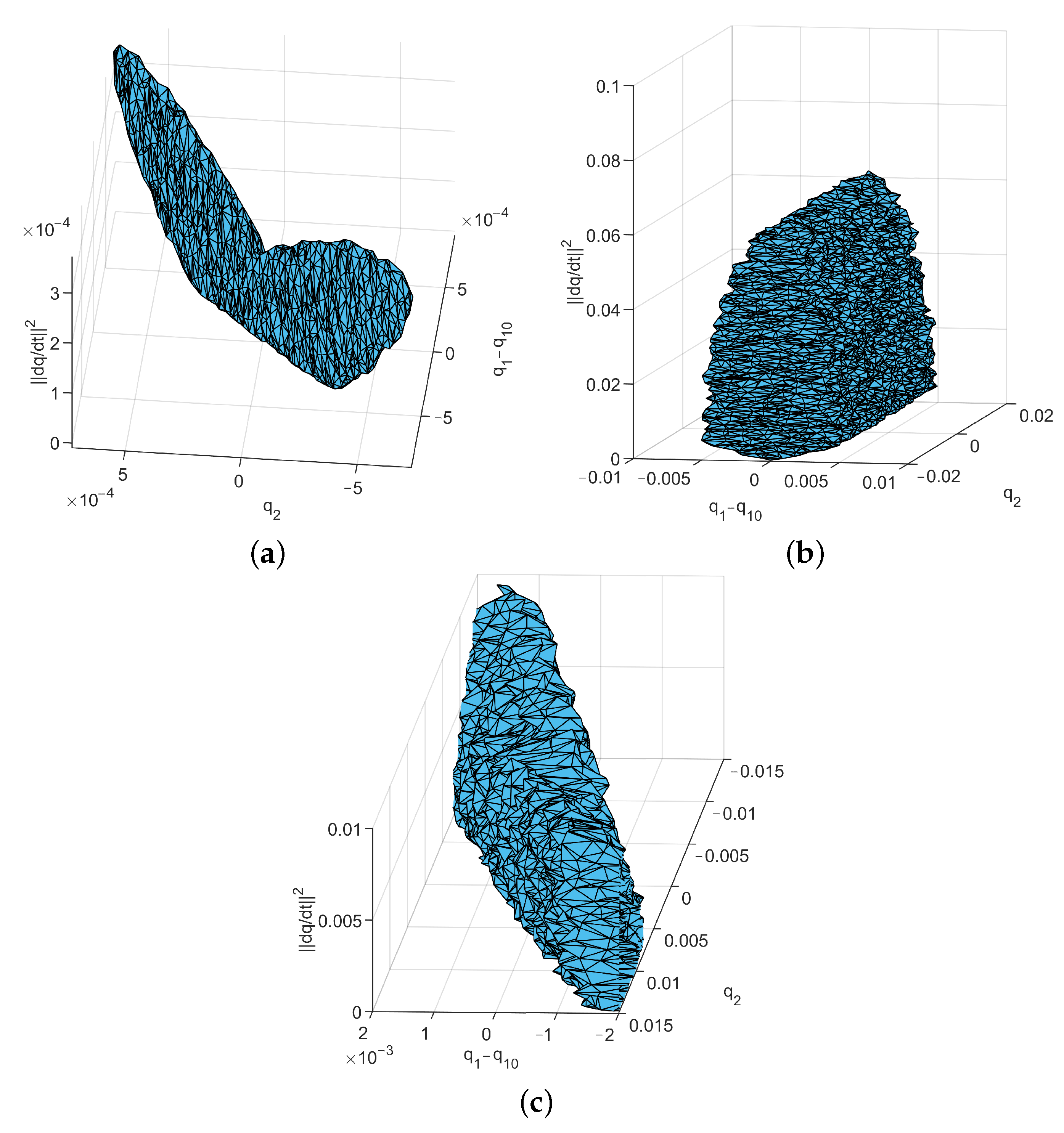
At first attempt the convergence sets where established taking into account Lyapunov analysis considered in the proof of the local exponential stability in Section 4.1. Lyapunov function (38) was chosen for each closed-loop system taking into account the original and transformed errors defined by $\tilde{x}$ and $\tilde{\xi }$, respectively. The quadratic bounds of the residual terms $r_1$ and $r_2$ were then numerically approximated in the assumed vicinity of the desired point. In this way, the constant C in (44) can be determined and the upper bound $\overline{V}$ can be computed. The set of feasible initial conditions can be found by searching for such states for which $V<\overline{V}$. The sets obtained in the three cases are roughly illustrated in Figure 3. Since the state space is 4-dimensional, the set cannot be visualized on a 2D figure. Therefore, two velocity components ${\dot{q}}_1$ and ${\dot{q}}_2$ are replaced by $∥\dot{q}∥$ presented on the z-axis.

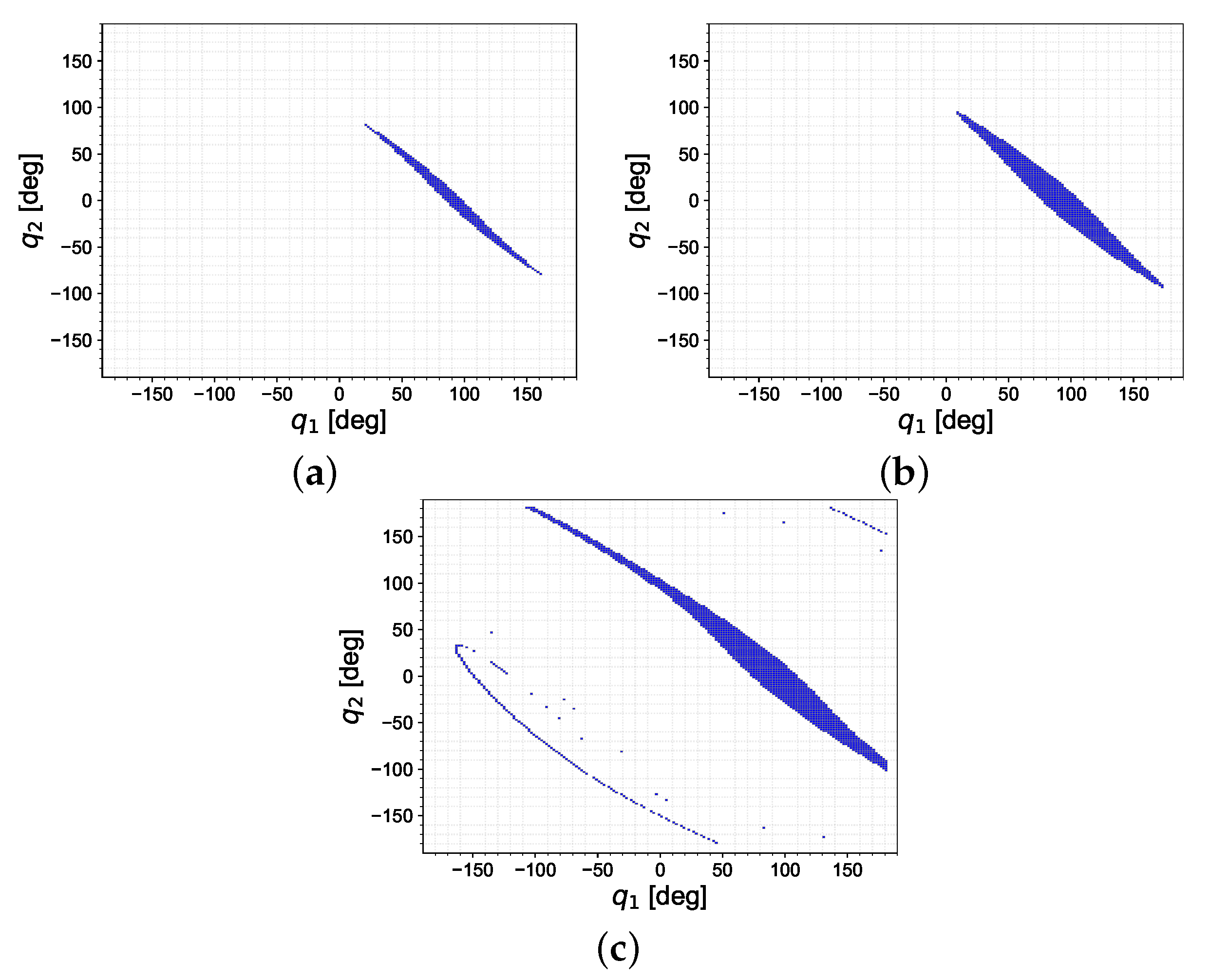
Although the obtained results confirm the local stability of the closed-loop systems, the main task of the research is to compare the attraction basin of each controller in more realistic conditions. To achieve such a comparison, the trajectories of closed-loop systems were evaluated. Such an analysis requires many simulation trails; thus, efficient implementation of simulation models is an important issue. As a result, simulations were carried out with the use of programming tools in the C++ language, including libraries for solving non-stiff differential equations.

For each controller, a discrete set of initial configurations is defined in the form of a two-dimensional grid. Each cell of the grid corresponds to an initial condition represented by $(q_1\left(0\right),q_2\left(0\right))$ and zero velocity $\omega \left(0\right)$. If, for the given condition, the state trajectory converges to the desired point, this trial is considered a positive result and the initial configuration considered is added to the set representing the basin of attraction. The results obtained are presented in Figure 4. Darker cells present an approximation of the basin of attraction, whereas white cells indicate that, for the corresponding initial condition, the control goal has not been accomplished properly.

Table 4. Comparison of areas occupied by the basin of attraction sets estimated based on numerical simulations.

Algorithm	Area [%]
$\Sigma$, (34)	1.10
${\Sigma }_{\mathrm{NQV}}^{*}$, (57)	2.91
${\Sigma }_{\mathrm{NF}}^{*}$, (57)	4.98

presents a comparison of the algorithms considered. The Area [%] index specifies the percentage of positive results related to the entire searched grid.

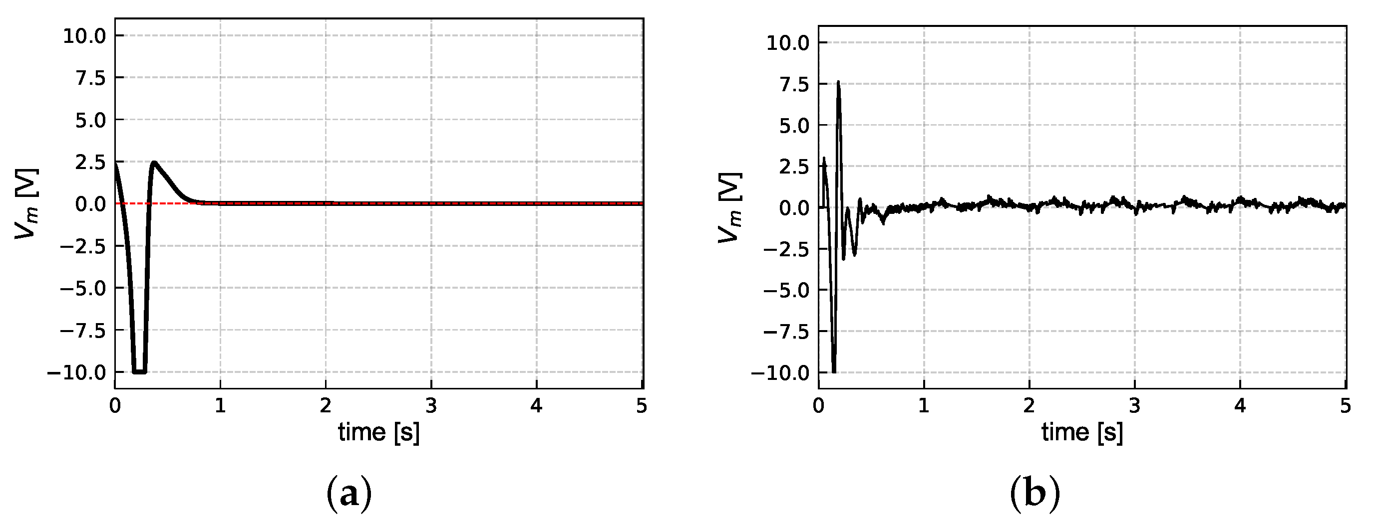
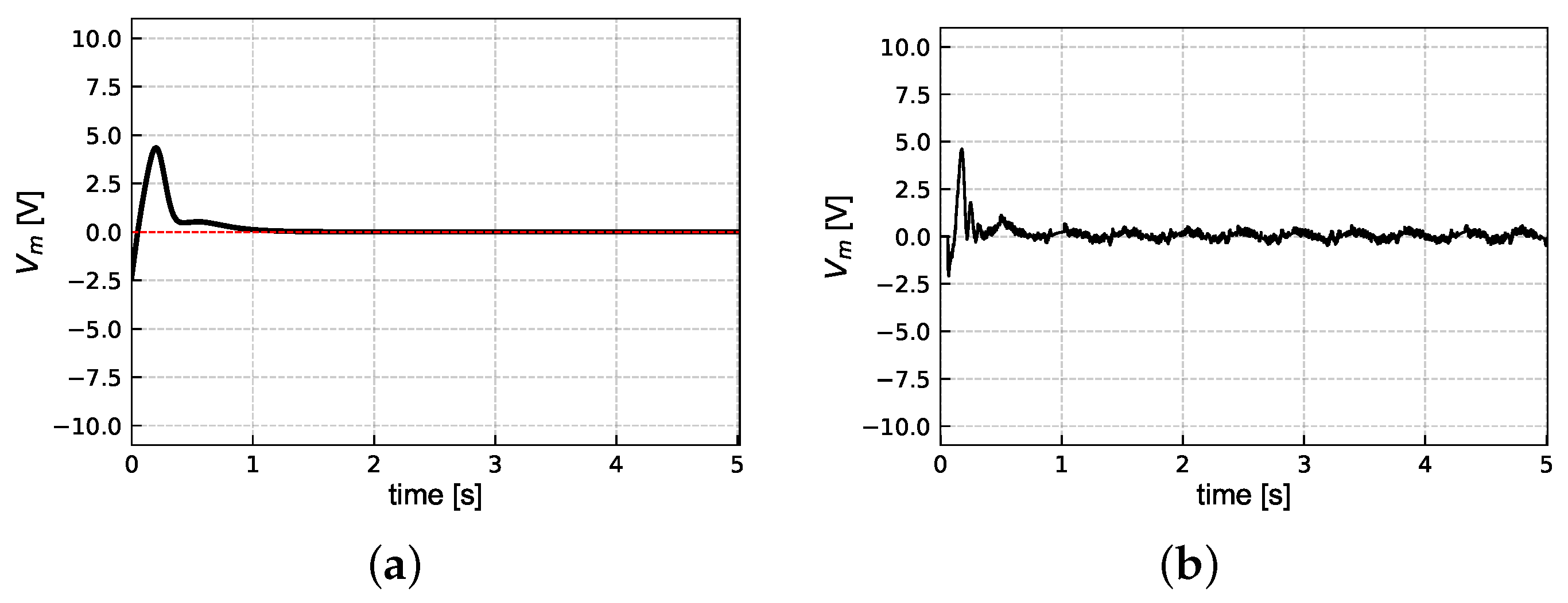
As part of the extended analysis, the waveforms of the robot configuration and the control input obtained during the simulations for the particular choice of initial configuration are presented along with the experimental results in Section 5.2. To facilitate a comparison between the simulation and the experimental results, the control input is represented by the motor voltage signal instead of the torque u. To further quantify the performance of each algorithm for the chosen initial condition, the index (32) is computed and presented in

Table 5. Comparison of values of performance index obtained for the same initial configuration.

Algorithm	$\mathcal{J}$
$\Sigma$, (34)	10.96
${\Sigma }_{\mathrm{NQV}}^{*}$, (57)	10.45
${\Sigma }_{\mathrm{NF}}^{*}$, (57)	11.21

.

5.2. Experiment

In the considered application for hardware implementation, a dedicated LabView environment and a driver with an amplifier provided by Quanser are used together with a PC computer, whose task is supervision, monitoring, and measurement registration.

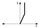
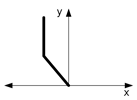
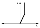
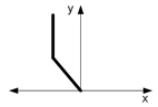
Taking into account the determined basin of attraction for each simulated algorithm, presented in Figure 4, an experimental verification of these algorithms was carried out for a particular selection of initial conditions that belong to the obtained sets. Two different initial postures of the Pendubot were selected. In Scenario 1 the Pendubot initially is tilted to the right, while in Scenario 2 it is tilted to the left. The desired point has been chosen according to (65). For each of the cases considered, a table containing the simulation and experiment conditions, as well as a schematic visualization of the robot initial position. Additionally, the table contains both the controller parameters used during the simulation and the corresponding settings used in the experiment. To make the presentation more clear, the following cases are distinguished:

• Case A: the linear controller designed for the nominal dynamics $\Sigma$ is used, see

  Table 6. Case A1: Initial posture of the Pendubot and parameters of the linear controller.

  Type		$\mathbf{\Sigma }$, (34)
  $(q_1\left(0\right),q_2\left(0\right))$		$(65,25)\mathrm{deg}$
  SIM:	K	$\{-10.4,-9.7,-2.5,-1.9\}$
  EXP:	K	$\{-9.8,-9,-0.6,-0.3\}$

  and

  Table 7. Case A2: Initial posture of the Pendubot and parameters of the linear controller.

  Type		$\mathbf{\Sigma }$, (34)
  $(q_1\left(0\right),q_2\left(0\right))$		$(130,-40)\mathrm{deg}$
  SIM:	K	$\{-10.4,-9.7,-2.5,-1.9\}$
  EXP:	K	$\{-10.4,-9.7,-2.5,-1.9\}$

  ;
• Case B: the nonlinear controller designed based on transformed dynamics ${\Sigma }_{\mathrm{NQV}}^{*}$ is used, see

  Table 8. Case B1: Initial posture of the Pendubot and parameters of the nonlinear controller.

  Type		${\mathbf{\Sigma }}_{\mathbf{NQV}}^{*}$, (57)
  $(q_1\left(0\right),q_2\left(0\right))$		$(65,25)\mathrm{deg}$
  SIM:	$K^{*}$	$\{-94,-88,26,-184\}$
  EXP:	$K^{*}$	$\{-150,-150,11,-100\}$

  and

  Table 9. Case B2: Initial posture of the Pendubot and parameters of the nonlinear controller.

  Type		${\mathbf{\Sigma }}_{\mathbf{NQV}}^{*}$, (57)
  $(q_1\left(0\right),q_2\left(0\right))$		$(130,-40)\mathrm{deg}$
  SIM:	$K^{*}$	$\{-94,-88,26,-184\}$
  EXP:	$K^{*}$	$\{-150,-150,11,-100\}$

  ;
• Case C: the nonlinear controller designed based on transformed dynamics ${\Sigma }_{\mathrm{NF}}^{*}$ is used, see

  Table 10. Case C1: Initial posture of the Pendubot and parameters of the nonlinear controller.

  Type		${\mathbf{\Sigma }}_{\mathbf{NF}}^{*}$, (57)
  $(q_1\left(0\right),q_2\left(0\right))$		$(65,25)\mathrm{deg}$
  SIM:	$K^{*}$	$\{-1187,-236,314,26\}$
  EXP:	$K^{*}$	$\{-1187,-130,314,8\}$

  and

  Table 11. Case C2: Initial posture of the Pendubot and parameters of the nonlinear controller.

  Type		${\mathbf{\Sigma }}_{\mathbf{NF}}^{*}$, (57)
  $(q_1\left(0\right),q_2\left(0\right))$		$(130,-40)\mathrm{deg}$
  SIM:	$K^{*}$	$\{-1187,-236,314,26\}$
  EXP:	$K^{*}$	$\{-1187,-130,314,8\}$

  .

6. Discussion

The simulation results obtained show that the LQR design, taking advantage of equivalent systems, can improve the attraction basin in the task of stabilizing the Pendubot. Based on the conservative estimation of attraction sets by the Lyapunov method, the attraction basin for the classical version of LQR is the most limited. This is due to the dependence of the input matrix on the state, which introduces additional nonlinearity, shown in (40). In contrast, for the transformed systems considered ${\Sigma }^{*}$, the input matrix is constant, leading to an increase in the attraction basin. It is worth noting that the largest volume of attraction set is obtained for system ${\Sigma }_{\mathrm{NQV}}^{*}$, which is defined in terms of inertial quasi-velocities.

The results of the convergence analysis, based on extensive simulations, see Figure 4, indicate that the considered Lyapunov-based method is too restrictive. Comparing the areas occupied by the cells corresponding to feasible initial configurations presented in Table 4 one can conclude that algorithms based on Formula (57) make it possible to increase the area of acceptable initial configurations from 2.5 to 4.5 times compared to the nominal case. It is interesting that the basin of attraction is the largest for the system ${\Sigma }_{\mathrm{NF}}^{*}$ while the Lyapunov-based analysis suggests better characteristics with respect to system ${\Sigma }_{\mathrm{NQV}}^{*}$.

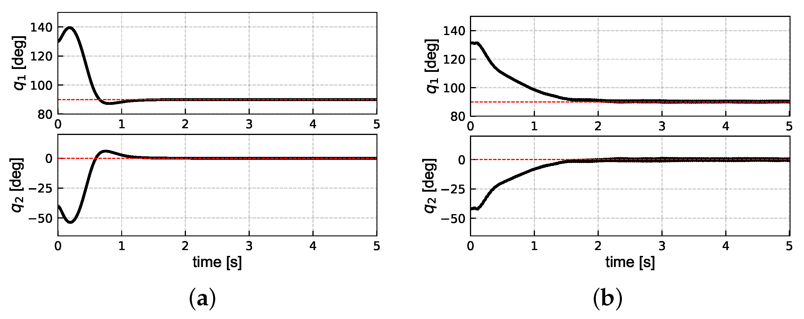
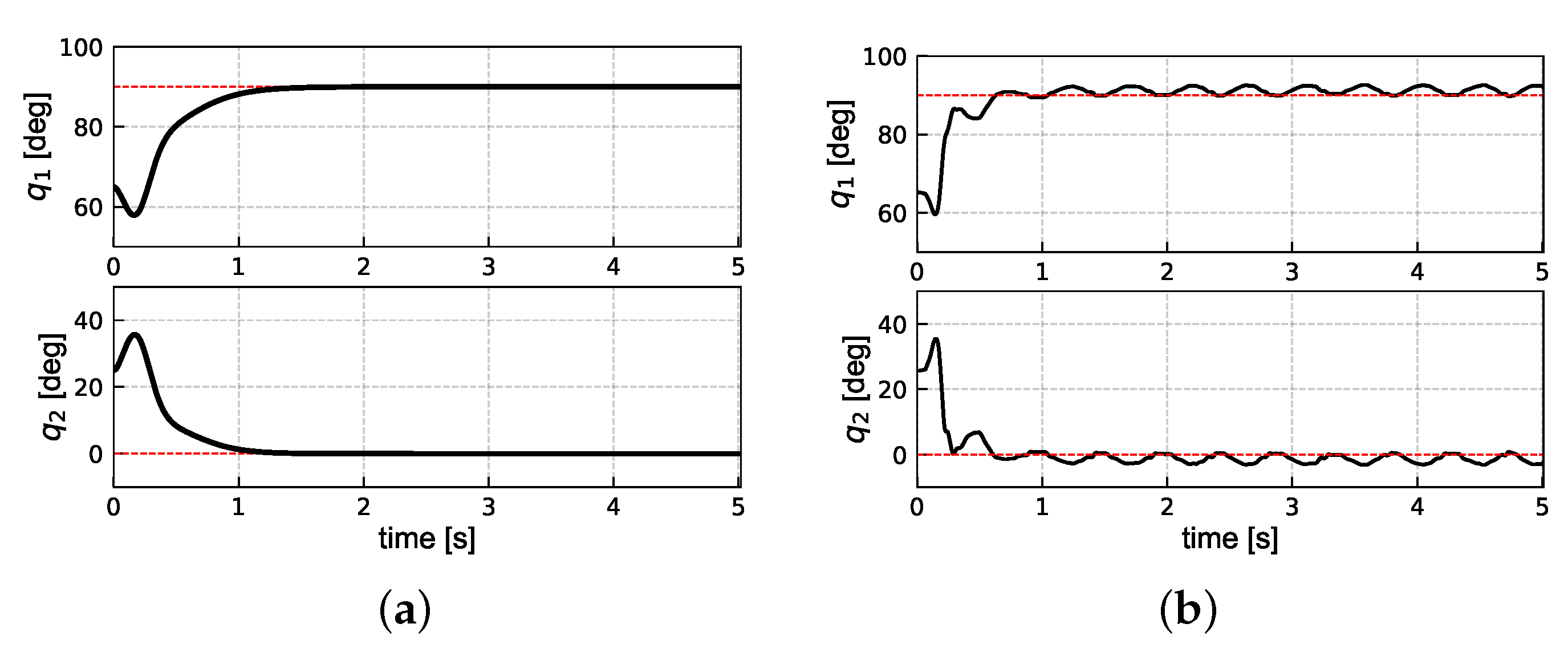
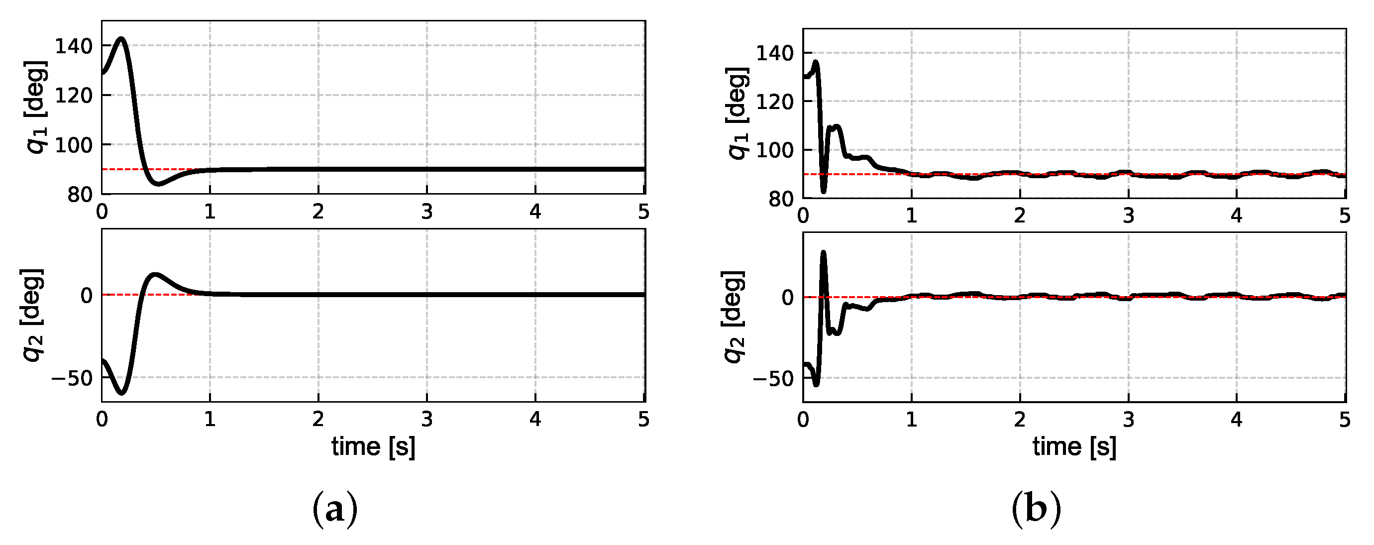
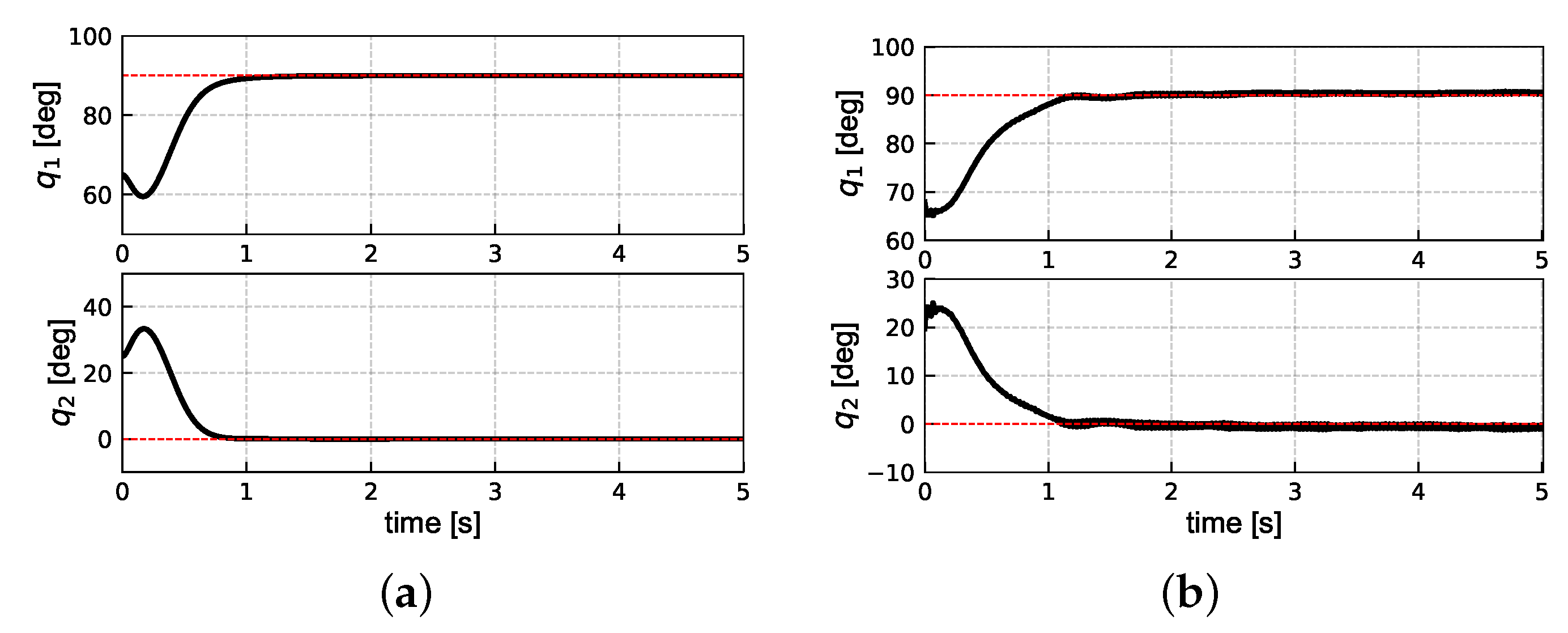
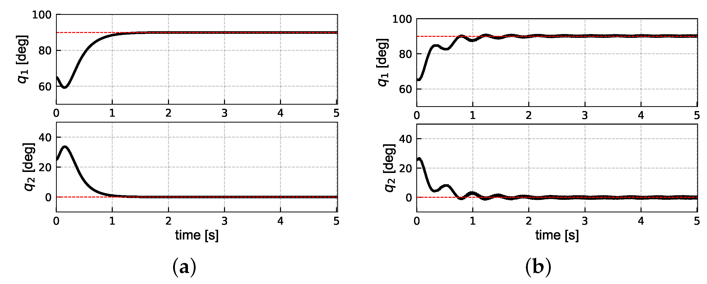
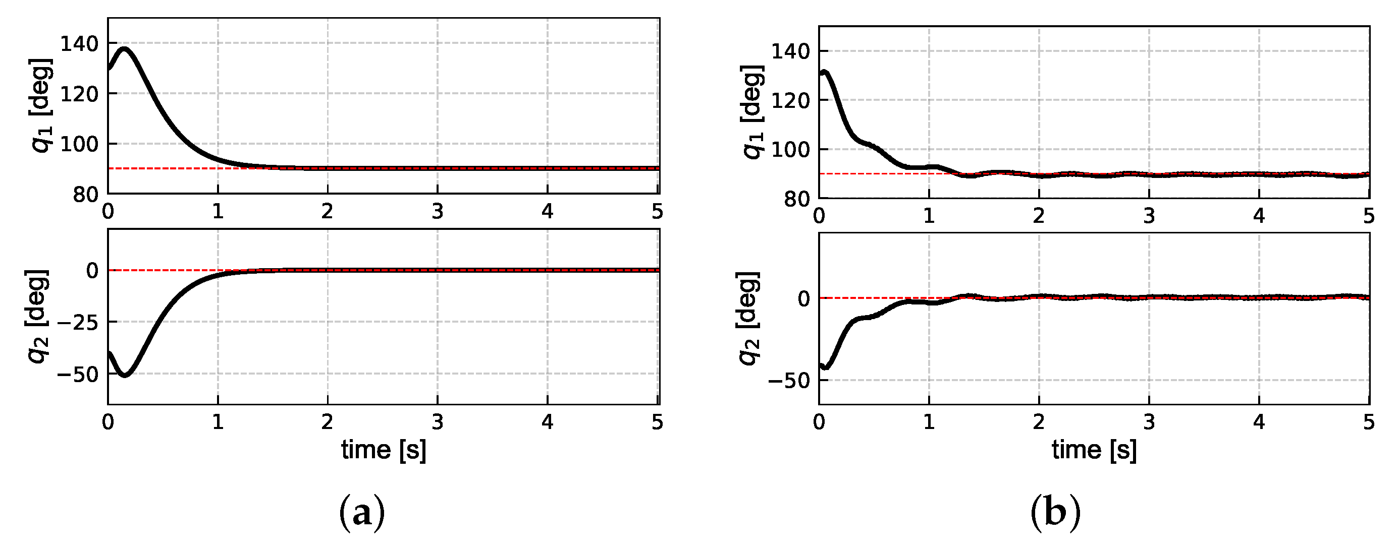
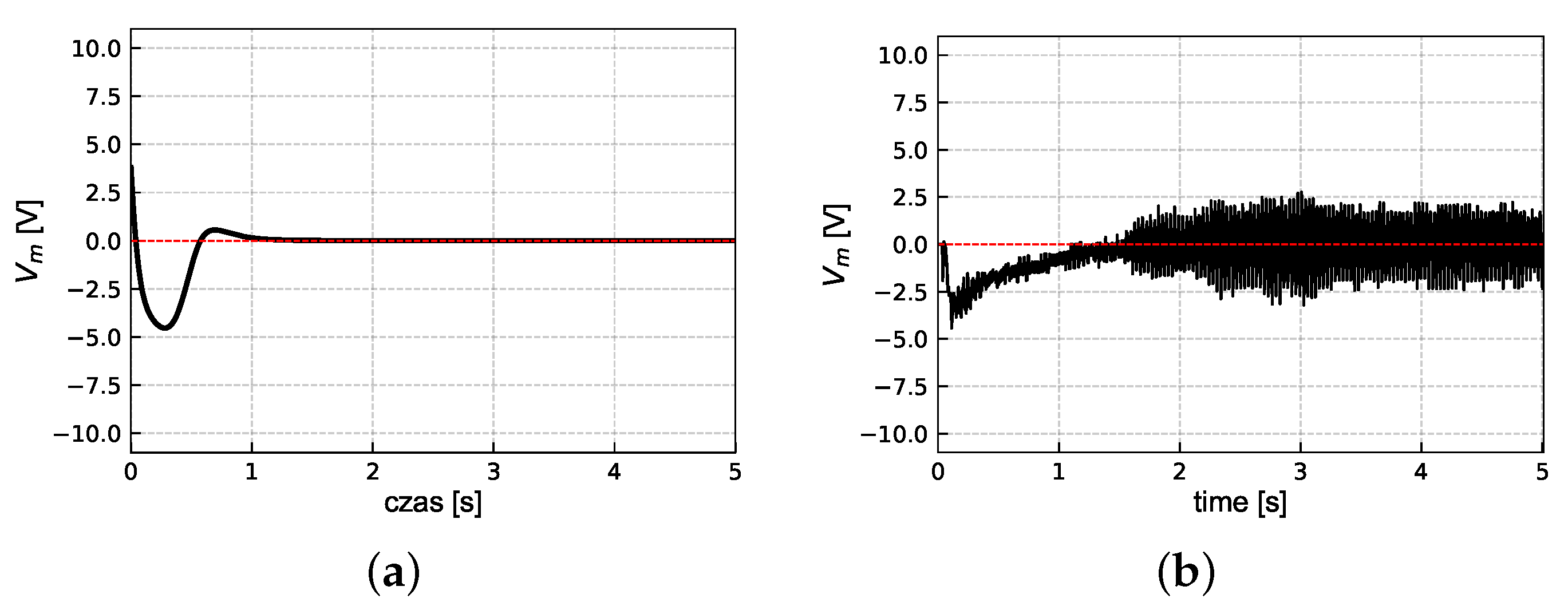
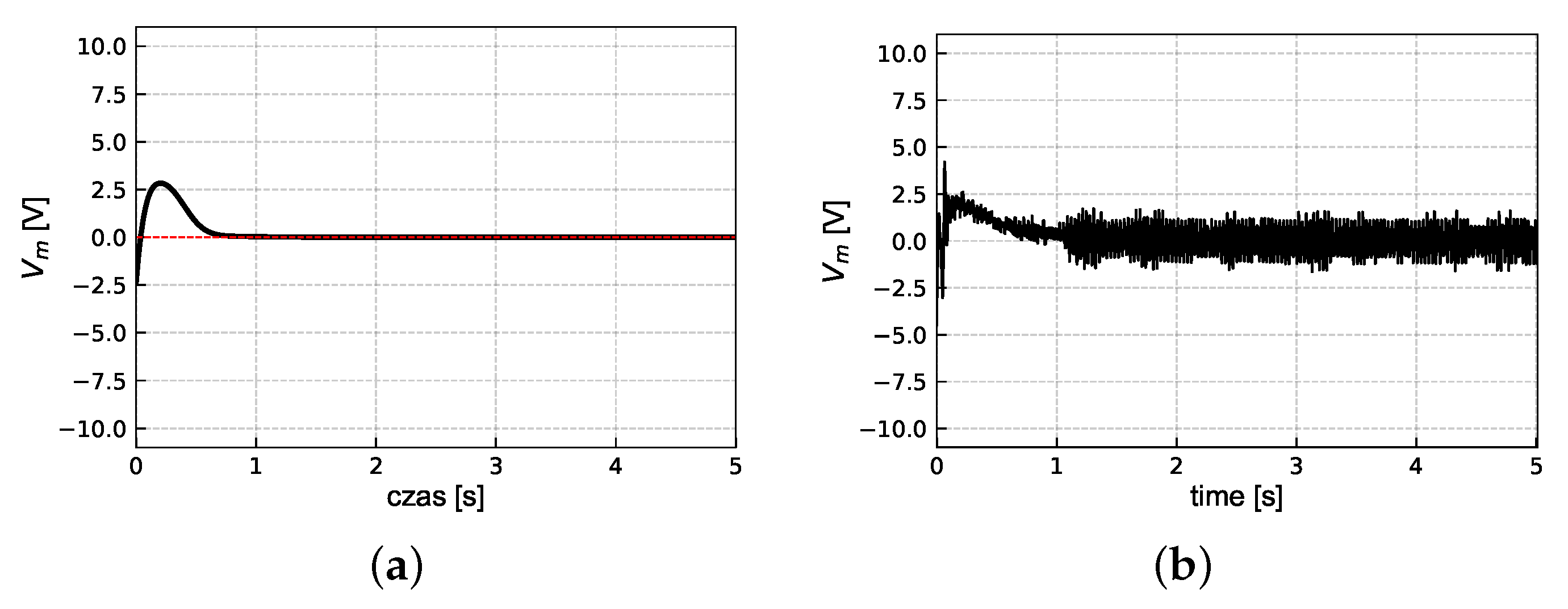
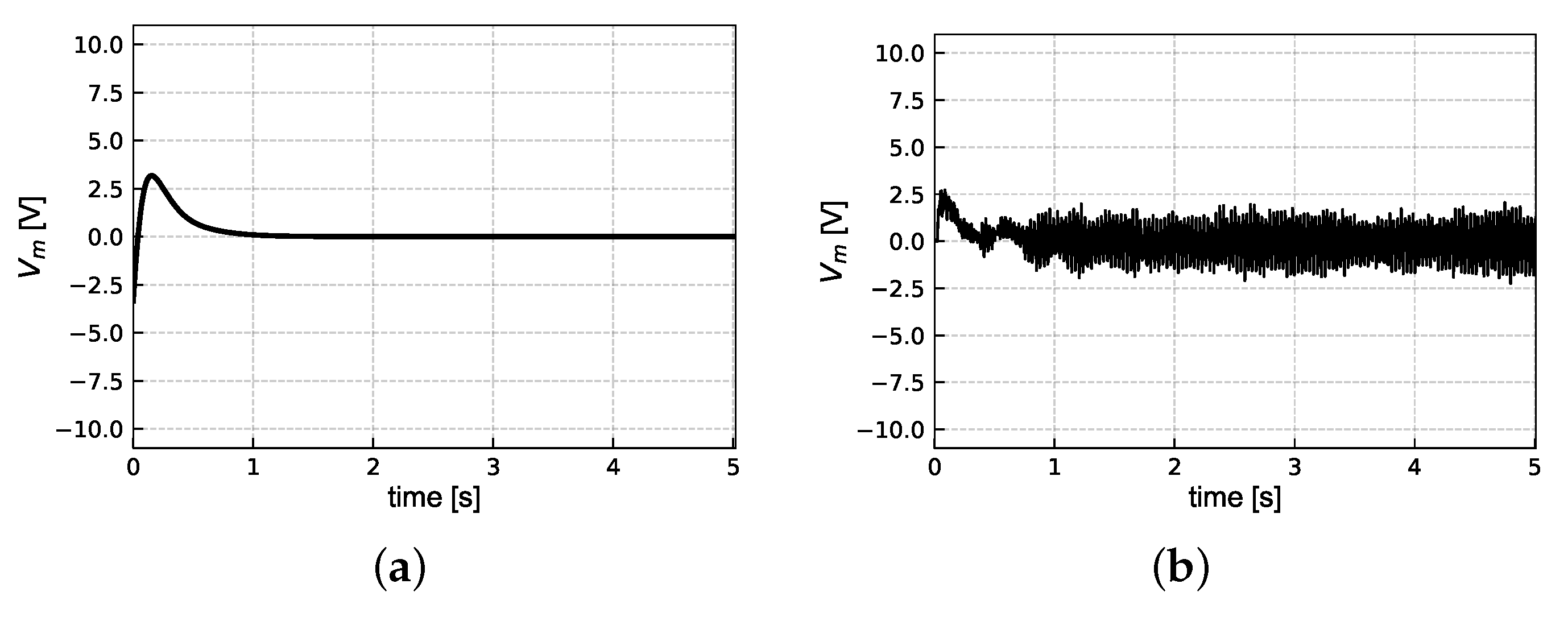
The results of the simulations performed for the same initial conditions and presented in Figure 5a, Figure 6a, Figure 7a, Figure 8a, Figure 9a, Figure 10a, Figure 11a, Figure 12a, Figure 13a, Figure 14a, Figure 15a, Figure 16a confirm that the step response of closed-loop systems is similar. However, comparing Figure 5a and Figure 7a with Figure 9a, Figure 11a, Figure 13a and Figure 15a more thoroughly, one can state that the transient response obtained for the nominal feedback more clearly exhibits the characteristics inherent in non-linear systems, while for the nonlinear controllers the time plots are smoother and even more characteristic for linear systems. A similar conclusion can be drawn with respect to the analysis of control inputs presented in Figure 6a, Figure 8a, Figure 10a, Figure 12a, Figure 14a and Figure 16a. Similar values of the performance index shown in Table 5 also confirm that the dynamics of the closed-loop system is preserved.

Based on the outcomes presented in Section 5.2, it can be seen that the simulation results and their counterparts obtained in experiments, cf. Figure 5a,b, Figure 6a,b, Figure 7a,b, Figure 8a,b, Figure 9a,b, Figure 10a,b, Figure 11a,b, Figure 12a,b, Figure 13a,b, Figure 14a,b, Figure 15a,b, Figure 16a,b, are fairly similar. Thus, one can cautiously conclude that the mathematical model used to describe the real system is quite close to it; however, some uncertainties can affect the results of the experiment. The similarity manifests itself in terms of the signal amplitudes, but time parameters such as the regulation time is in most cases is longer during experiment. The differences can be explained by the occurrence of effects omitted in the object dynamics model, which include, e.g., static and dynamic friction (occurring in the drive system as well as during the influence of aerodynamic phenomena), backlash and spring effects, and measurement uncertainties. It was observed that the resolutions of the encoders were not enough to obtain high-quality velocity estimates. In particular, the velocity of the second joint cannot be accurately estimated. Taking into account these limitations, adjustments to the gains were required to ensure proper operation of the real system. Especially, in experiments it was necessary to decrease gains associated with velocity components due to the impact of insufficient quality of the velocity estimation. However, decreasing these gains introduces a higher oscillatory response of the closed-loop system, which can be clearly observed in Figure 5, Figure 7 and Figure 13.

In the simulation and experimental tests under consideration, attention should also be paid to the problem of input saturation, which has a significant impact on the attraction set. Despite this, it can be seen that even under input signal constraints, the alternative representation of the dynamics enlarges the convergence set.

There is another issue worth highlighting. Namely, the application of variable transformation may also have the negative effect of increasing the sensitivity of the control system to measurement noise. This may explain the appearance of higher noise in the input signal u for the cases including transformations (cf. Figure 10b, Figure 12b, Figure 14b and Figure 16b) than for the nominal case (cf. Figure 6b and Figure 8b).

7. Conclusions

This paper considers the issue of LQR design for nonlinear systems using a smooth state and input transformation. The proposed design methodology is considered in the Pendubot stabilization task. The properties of the controllers studied were investigated in a simulation environment using experimental tests. Despite some limitations and technical imperfections of the experimental stand, one can conclude that the considered methods to some extent are robust to unmodelled effects and make it possible to provide satisfactory results in real applications.

The results of the tests carried out allow for a hypothesis that the controller using quasi-velocities allows one to increase the range of stabilizer convergence while maintaining the same dynamics of the closed system at the desired point. This property results from the introduction of nonlinearities in the stabilizer equation, which have a positive effect on the properties of the closed-loop system.

To the best of the authors’ knowledge, this work compares for the first time the properties of LQR controllers using different representations of Pendubot dynamics. The detailed forms of transformations and linear approximations given can be regarded as ready-made procedures that can be applied to stabilize similar mechanical systems in robotics.

In the future, the control methodology discussed in this paper can be applied for trajectory tracking, making it possible to also consider swing-up control problems addressed for a class of underactuated systems.

References

1. Kalman, R. Contributions to the theory of optimal control. Bol. Soc. Mat. Mex. 1960, 5, 102–119. [Google Scholar]
2. Khalil, H. Nonlinear Systems; Prentice Hall: Upper Saddle River, NJ, USA, 1996. [Google Scholar]
3. Wang, Y.; Zhang, Z.; Li, C.; Buss, M. Adaptive incremental sliding mode control for a robot manipulator. Mechatronics 2022, 82, 102717. [Google Scholar] [CrossRef]
4. Cunha, A.; Shao, M.; Huang, Y.; Silberschmidt, V.V. Intelligent Manipulator with Flexible Link and Joint: Modeling and Vibration Control. Shock Vib. 2020, 2020, 4671358. [Google Scholar] [CrossRef] [Green Version]
5. Batista, J.G.; Souza, D.A.; dos Reis, L.L.; Filgueiras, L.V.; Ramos, K.M.; Junior, A.B.; Correia, W.B. Performance Comparison Between the PID and LQR Controllers Applied to a Robotic Manipulator Joint. In Proceedings of the IECON 2019—45th Annual Conference of the IEEE Industrial Electronics Society, Lisbon, Portugal, 14–17 October 2019; Volume 1, pp. 479–484. [Google Scholar] [CrossRef]
6. Mason, S.; Righetti, L.; Schaal, S. Full dynamics LQR control of a humanoid robot: An experimental study on balancing and squatting. In Proceedings of the 2014 IEEE-RAS International Conference on Humanoid Robots, Madrid, Spain, 18–20 November 2014; pp. 374–379. [Google Scholar] [CrossRef]
7. Xin, X.; Tanaka, S.; She, J.; Yamasaki, T. New analytical results of energy-based swing-up control for the Pendubot. Int. J. Non-Linear Mech. 2013, 52, 110–118. [Google Scholar] [CrossRef]
8. Toan, T.V.; Ha, T.T.; Do, T.V. Hybrid control for swing up and balancing pendubot system: An experimental result. In Proceedings of the 2017 International Conference on System Science and Engineering (ICSSE), Ho Chi Minh City, Vietnam, 21–23 July 2017; pp. 450–453. [Google Scholar] [CrossRef]
9. Leines, M.T.; Yang, J.S. LQR control of an under actuated planar biped robot. In Proceedings of the 2011 6th IEEE Conference on Industrial Electronics and Applications, Beijing, China, 21–23 June 2011; pp. 1684–1689. [Google Scholar] [CrossRef]
10. Alcala, E.; Puig, V.; Quevedo, J.; Escobet, T.; Comasolivas, R. Autonomous vehicle control using a kinematic Lyapunov-based technique with LQR-LMI tuning. Control Eng. Pract. 2018, 73, 1–12. [Google Scholar] [CrossRef]
11. Çimen, T. State-Dependent Riccati Equation (SDRE) Control: A Survey. IFAC Proc. Vol. 2008, 41, 3761–3775. [Google Scholar]
12. Bernat, J.; Kołota, J.; Stępień, S.; Superczyńska, P. Suboptimal control of nonlinear continuous-time locally positive systems using input-state linearization and SDRE approach. Bull. Pol. Acad. Sci. Tech. Sci. 2018, 66, 17–22. [Google Scholar] [CrossRef]
13. Stępień, S.; Superczyńska, P. Modified Infinite-Time State-Dependent Riccati Equation Method for Nonlinear Affine Systems: Quadrotor Control. Appl. Sci. 2021, 11, 10714. [Google Scholar] [CrossRef]
14. Giernacki, W.; Stępień, S.; Chodnicki, M.; Wróblewska, A. Hybrid Quasi-Optimal PID-SDRE Quadrotor Control. Energies 2022, 15, 4312. [Google Scholar] [CrossRef]
15. Jacobsen, D.; Mayne, D. Differential Dynamic Programming; Elsevier: New York, NY, USA, 1970. [Google Scholar]
16. Theodorou, E.; Tassa, Y.; Todorov, E. Stochastic Differential Dynamic Programming. In Proceedings of the 2010 American Control Conference, Baltimore, MD, USA, 30 June–2 July 2010; pp. 1125–1132. [Google Scholar] [CrossRef] [Green Version]
17. Li, W.; Todorov, E. Iterative Linear Quadratic Regulator Design for Nonlinear Biological Movement Systems. In Proceedings of the the First International Conference on Informatics in Control, Automation and Robotics (ICINCO), Setúbal, Portugal, 25–28 August 2004; Araújo, H., Vieira, A., Braz, J., Encarnação, B., Carvalho, M., Eds.; pp. 222–229. [Google Scholar]
18. Van den Berg, J. Iterated LQR smoothing for locally-optimal feedback control of systems with non-linear dynamics and non-quadratic cost. In Proceedings of the 2014 American Control Conference, Portland, OR, USA, 4–6 June 2014; pp. 1912–1918. [Google Scholar] [CrossRef]
19. Respondek, W. Feedback classification of nonlinear control systems on R2 and R3. In Geometry of Feedback and Optimal Control; Jakubczyk, B., Respondek, W., Eds.; Dekker: New York, NY, USA, 1998; pp. 347–381. [Google Scholar]
20. Jakubczyk, B.; Respondek, W. On linearization of control systems. Bull. Acad. Polon. Sci. Ser. Sci. Math. 1980, 28, 517–522. [Google Scholar]
21. Hammami, M.; Rettab, N. On the region of attraction of dynamical systems: Application to Lorenz equations. Arch. Control Sci. 2020, 30, 389–409. [Google Scholar] [CrossRef]
22. Zhao, K. Local exponential stability of four almost-periodic positive solutions for a classic Ayala-Gilpin competitive ecosystem provided with varying-lags and control terms. Int. J. Control 2022, 1, 1–13. [Google Scholar] [CrossRef]
23. Valmorbida, G.; Anderson, J. Region of attraction estimation using invariant sets and rational Lyapunov functions. Automatica 2017, 75, 37–45. [Google Scholar] [CrossRef] [Green Version]
24. El-Guindy, A.; Han, D.; Althoff, M. Estimating the region of attraction via forward reachable sets. In Proceedings of the 2017 American Control Conference (ACC), Seattle, WA, USA, 24–26 May 2017; pp. 1263–1270. [Google Scholar] [CrossRef] [Green Version]
25. Ziętkiewicz, J. Linear quadratic control with feedback-linearized models. Stud. Autom. Inf. Technol. 2015, 40, 37–49. [Google Scholar]
26. Owczarkowski, A.; Horla, D.; Zietkiewicz, J. Introduction of Feedback Linearization to Robust LQR and LQI Control—Analysis of Results from an Unmanned Bicycle Robot with Reaction Wheel. Asian J. Control 2019, 21, 1028–1040. [Google Scholar] [CrossRef]
27. Spong, M.; Block, D. The Pendubot: A mechatronic system for control research and education. In Proceedings of the 1995 34th IEEE Conference on Decision and Control, New Orleans, LA, USA, 13–15 December 1995; Volume 1, pp. 555–556. [Google Scholar] [CrossRef]
28. Prasad, L.B.; Tyagi, B.; Gupta, H.O. Optimal Control of Nonlinear Inverted Pendulum System Using PID Controller and LQR: Performance Analysis Without and With Disturbance Input. Int. J. Autom. Comput. 2014, 11, 661–670. [Google Scholar] [CrossRef] [Green Version]
29. Cimborová, K.; Jadlovská, S. Modeling of benchmark underactuated systems via different approaches. IFAC-PapersOnLine 2020, 53, 8935–8940. [Google Scholar] [CrossRef]
30. Li, S.; Moog, C.; Respondek, W. Maximal feedback linearization and its internal dynamics with applications to mechanical systems on R4. Int. J. Robust Nonlinear Control 2019, 29, 2639–2659. [Google Scholar] [CrossRef]
31. Parulski, P.; Bartkowiak, P.; Pazderski, D. Evaluation of Linearization Methods for Control of the Pendubot. Appl. Sci. 2021, 11, 7615. [Google Scholar] [CrossRef]
32. Meirovitch, L. Methods of Analytical Dynamics; McGraw–Hill: New York, NY, USA, 1970. [Google Scholar]
33. Gutowski, R. Mechanika Analityczna; PWN: Warsaw, Poland, 1971. [Google Scholar]
34. Jain, A.; Rodriguez, G. Diagonalized Lagrangian robot dynamics. IEEE Trans. Robot. Autom. 1995, 11, 571–584. [Google Scholar] [CrossRef]
35. Rodriguez, G.; Jain, A.; Kreutz-Delgado, K. A Spatial Operator Algebra for Manipulator Modeling and Control. Int. J. Robot. Res. 1991, 10, 371–381. [Google Scholar] [CrossRef] [Green Version]
36. Herman, P. A controller of the pendubot using quasi-velocities. In Proceedings of the 2008 16th MED Conference, Vancouver, BC, Canada, 27–31 October 2008; pp. 1066–1070. [Google Scholar] [CrossRef]
37. Olfati-Saber, R. Nonlinear Control of Underactuated Mechanical Systems with Application to Robotics and Aerospace Vehicles. Ph.D. Thesis, Massachusetts Institute of Technology, Cambridge, MA, USA, 2001. AAI0803036. [Google Scholar]
38. Olfati-Saber, R. Normal forms for underactuated mechanical systems with symmetry. IEEE Trans. Autom. Control 2002, 47, 305–308. [Google Scholar] [CrossRef] [Green Version]
39. Spong, M.W. Partial feedback linearization of underactuated mechanical systems. In Proceedings of the IEEE/RSJ International Conference on Intelligent Robots and Systems (IROS’94), Munich, Germany, 12–16 September 1994; Volume 1, pp. 314–321. [Google Scholar]
40. Kwakernaak, H.; Sivan, R. Linear Optimal Control System; Wiley-Interscience: New York, NY, USA, 1972. [Google Scholar]
41. Nowicki, M.; Respondek, W. A Mechanical Feedback Classification of Linear Mechanical Control Systems. Appl. Sci. 2021, 11, 10669. [Google Scholar] [CrossRef]
42. Quanser. Rotary Double Inverted Pendulum. Available online: www.quanser.com/products/rotary-double-inverted-pendulum/ (accessed on 12 July 2022).
Figure 1. Scheme of the Pendubot: (a) basic model: m i —mass of i th link, I i —moment of inertia of i th link determined with respect to the axis normal to the plane and moving through the center of mass of the link, l i —length of i th link, l c i —distance between the revolute joint and the center of mass of i th link, g—gravity acceleration, (b) the real system used in experimental research.
Energies 15 05146 g001
Figure 2. Locally equivalent control structures (linear parts are denoted by dotted lines): (a) Classical linear controller, (b) Nonlinear controller using linear feedback in new set of coordinates.
Energies 15 05146 g002
Figure 3. Area of convergence estimated in a conservative way based on the Lyapunov analysis: (a) Σ , (b) Σ NQV * , (c) Σ NF * .
Energies 15 05146 g003
Figure 4. Area of convergence: (a) Σ , (b) Σ NQV * , (c) Σ NF * .
Energies 15 05146 g004
Figure 5. Case A1: Angular positions: (a) simulation, (b) experiment.
Energies 15 05146 g005
Figure 6. Case A1: Input signal: (a) simulation, (b) experiment.
Energies 15 05146 g006
Figure 7. Case A2: Angular positions: (a) simulation, (b) experiment.
Energies 15 05146 g007
Figure 8. Case A2: Input signal: (a) simulation, (b) experiment.
Energies 15 05146 g008
Figure 9. Case B1: Angular positions: (a) simulation, (b) experiment.
Energies 15 05146 g009
Figure 10. Case B1: Input signal: (a) simulation, (b) experiment.
Energies 15 05146 g010
Figure 11. Case B2: Angular positions: (a) simulation, (b) experiment.
Energies 15 05146 g011
Figure 12. Case B2: Input signal: (a) simulation, (b) experiment.
Energies 15 05146 g012
Figure 13. Case C1: Angular positions: (a) simulation, (b) experiment.
Energies 15 05146 g013
Figure 14. Case C1: Input signal: (a) simulation, (b) experiment.
Energies 15 05146 g014
Figure 15. Case C2: Angular positions: (a) simulation, (b) experiment.
Energies 15 05146 g015
Figure 16. Case C2: Input signal: (a) simulation, (b) experiment.
Energies 15 05146 g016