1. Introduction
The vortex generated around the suction region of the pump sump causes adverse effects such as the deterioration of pump performance and deviations in operating conditions [
1,
2,
3,
4,
5]. If a flow imbalance occurs in the water reservoir, this causes a swirling flow around the sump intake, reducing the efficiency and stability of the pump. Although ASME HI 9.8 Standard 2018 [
6] does not recommend vortices prediction via computational fluid dynamics (CFD), it is frequently performed because of the high industry demand to reduce model testing time and cost. In the study by Choi et al., the location of the vortex was predicted using CFD techniques [
7]. In addition, CFD was used to analyze the swirl angle, which was used to determine the imbalance of the water returned to the pump through the bell-mouth by Ayham Amin et al. [
8,
9]. As such, the prediction of pump sump performance using CFD techniques has been carried out effectively, but it is difficult to predict the free surface vortices and sub-surface vortices using CFD under the ASME HI 9.8 standard. For this reason, it is impossible to define the vortex types by analyzing the CFD results alone, but with the sump test, it is possible to approach these tasks conservatively [
6,
10].
Experiments using PIV technology have problems such as the visualization of a limited number of particles, the reflection of diffuse particles, and the limitations of the grids used in the post-processing program. Therefore, comparing the results of limited PIV data and CFD is inevitably accompanied by errors [
11,
12,
13,
14]. Nevertheless, CFD simulations are necessary for pump sump models since it is more useful if a standard range or vortex level values are presented.
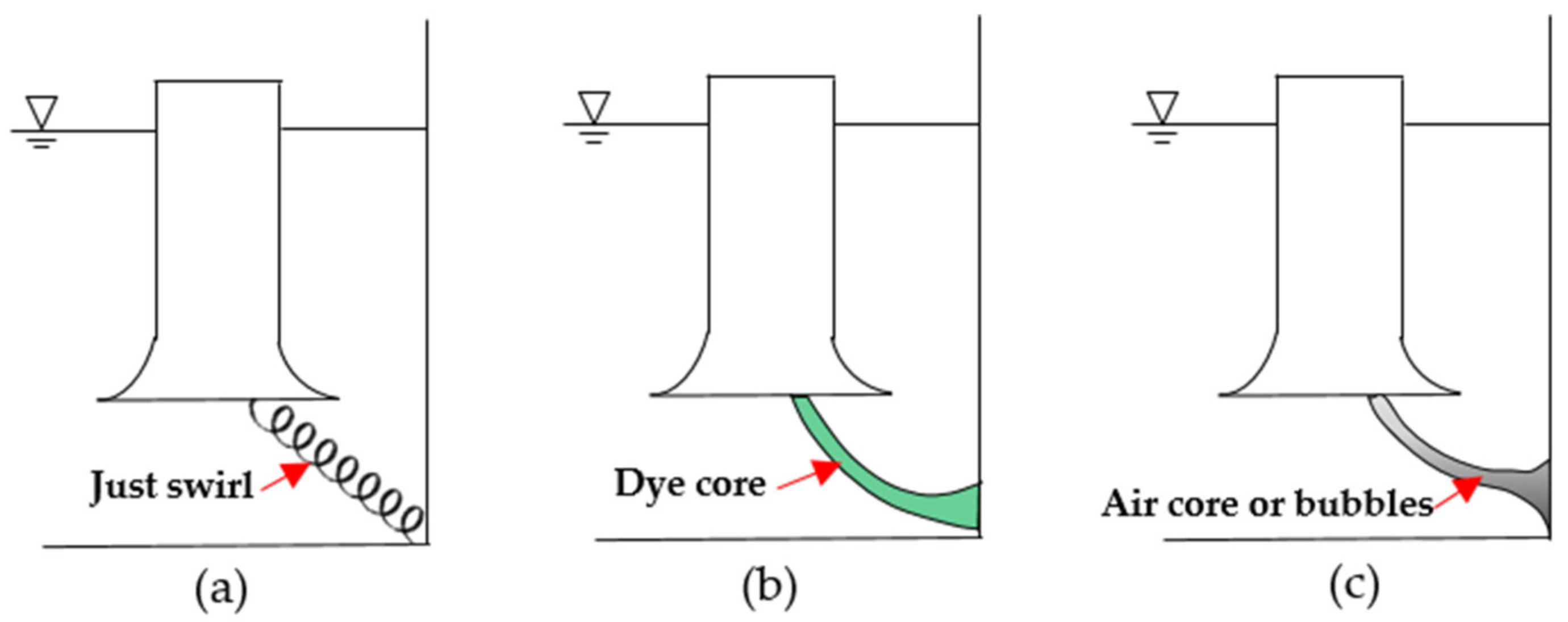
The vortices generated by the pump sump can be divided into free surface vortices and subsurface vortices. Furthermore, subsurface vortices are classified in
Figure 1 based on the level of vortex strength as Type 1, Type 2 and Type 3. In the case of Type 1 subsurface vortex, a simple swirl occurs, and the dye does not enter the bell-mouth, even if the swirl is recognized through the dye test. Subsurface vortices of Type 2 can be clearly visualized through the dye test, in which the generated vortex core flows into the bell-mouth. Even in the absence of the dye test, Type 3 subsurface vortices can be recognized since the vortex core visualizes the air or bubble flow into the bell-mouth [
6]. When the subsurface vortex exceeds Type 1, the pump sump was identified as an inappropriate design which the design should be improved using modifications such as AVD (anti-vortex devices).
CFD analysis was carried out on pump sumps to compare the swirl angle with tangential velocity analysis and confirm the uniform flow into the bell-mouth. Moreover, CFD was used to optimize the design of the pumping station by observing the CFD flow field around the AVD. Ayham Amin et al. claim that subsurface vortices can be generated in specific areas and can even have an adverse effect when the swirl angle is 5° or less, even though these cases are according to the standard value [
6,
8]. At this point, the type of the generated vortex cannot be defined without the CFD, so the AVD design is as conservative as possible [
15].
This study focuses on analyzing the subsurface vortex generation of Type 2 in the model test in terms of vorticity as well as vortex core area and location using CACTUS Ver.3.3, which is a commercial program that post-processes PIV results taken with a high-speed camera [
16]. Then, the model test results are compared with different CFD methods using Ansys CFX 17.2, a commercial CFD program. We tried to find the correlation between the model test and CFD through analysis of the subsurface vortex in terms of vorticity, indicating the strength of the swirl.
2. Model Test Method
Even though there are several pumps lined up in pumping stations, a single-channeled pump sump was used in this study. The experimental flow channel is made of acrylic material 4 m in length, 0.5 m in width, and 0.8 m in height. The sump test maintained the flow rate at 153.5 m
3/h. In the pump sump test model, the flow distributor is introduced to facilitate the generation of vortices by artificially causing a flow biased to one side [
10], which is fabricated to match the length and width of the short channel.
Figure 2a shows the experimental set-up indicating the main components, whereas
Figure 2b illustrates the flow distributor and
Figure 2c illustrates the dimensions of the flow distributor.
Experimental flow behavior was analyzed based on the PIV’s (particle image velocimetry) visualization technology and digital image processing technology. PIV is a method that obtains velocity vectors at multiple points simultaneously by tracing the particles in two images [
17]. For PIV measurements, polyvinyl chloride tracer particles with an average diameter of 100 µm were seeded in the water. These particles had a specific gravity of 1.02, similar to the water, resulting in even distribution in the flow field. An air-cooled DPSS (diode-pumped solid-state) was used to create a continuous laser sheet with an output of 4 W to illuminate the particles. A laser sheet was used to illuminate the PIV particles since the normal light beams reflect air bubbles interfering with the light path during image recording [
18]. A Photron CCD camera was used to capture the motion of the particles. The maximum fps (frame per second) of the camera is 10,000, and the camera has a pixel resolution of 1024 × 1024. The camera was installed on the left side of the flow channel. Since the experiment was conducted under low-light conditions, 250 fps was selected to illuminate the PIV particles in the laser sheet to have a clear resolution [
19,
20]. The images captured by the CCD camera were then processed using Cactus ver.3.3 using the grey-level cross-correlation algorithm for particle tracking [
21].
Figure 3 shows the PIV setup at the experiment, and
Table 1 lists the specifications of the devices used in PIV measurements.
3. Dye Test and PIV Post-Process
The PIV technology could capture the spatially and temporally resolved velocity measurements on the flow plane [
22]. The subsurface vortices of Type 2 were generated by the flow distributor along the left wall of the channel. Therefore, the generated vortices can be observed on the cross-section plane, which is 10 mm away from the left wall.
Figure 4 visualizes the PIV post-processed streak line results on the cross-section plane. It can see the dynamic behavior of the subsurface vortex of Type 2 since the vortices change their shape and location. The area beneath the bell-mouth was prioritized where the highest vorticity was recorded using averaged data.
Since the vorticity (ζ) is directly related to the strength of rotation, it was used to analyze the subsurface vortices of both the PIV and CFD results. Equation (1) is the formula for the vorticity and uses the velocity vectors on the 2D plane [
23]:
Initially, the model test was allowed to be stable from the beginning before taking the measurements. After the sump test was stable, showing periodic behavior, subsurface vortex formation of Type 2 was determined by comparing the time series dye test results with the post-processed vorticity results in PIV, as shown in
Figure 5. Vortex formation is periodic in most sump test studies [
15,
24,
25], whereas the observed subsurface vortex of Type 2 in this study followed a periodic pattern with a 2.56 s time period. The period pattern includes the appearance, maintenance and disappearance of the Type 2 subsurface vortices, whereas there is a period of absence of the subsurface vortices before they appear again. The periodic pattern is visualized in the dye test over a long period, whereas the PIV post-process mainly focuses on one cycle. This period pattern was used to compare the dye test results with the PIV vorticity contours in the time series. As shown in
Figure 5a, the subsurface vortices of Type 2 were determined with the dye test (the dye core entered the bell-mouth), whereas the PIV vorticity was higher than 63.8 (1/s). After the half-cycle was completed, the subsurface vortices of Type 2 disappeared, as shown in
Figure 5b. In the absence of Type 2 subsurface vortices, the lowest vorticity value is recorded as less than 56.6 (1/s). Therefore, 60.2 (1/s) was estimated as the average value for the formation of subsurface vortices of Type 2. Hence, the Type 2 subsurface vortex analysis in PIV and CFD data is based on the 60.2 (1/s) reference level where the Type 2 subsurface vortex core appears in the dye test results.
4. CFD Simulation Setup
The fluid domain for the single-channel and the bell-mouth were modeled and meshed, as shown in
Figure 6. The mesh at the main focus area was extra refined, while the near-wall treatment is used both at the channel wall and bell-mouth.
Figure 6a shows the boundary conditions for CFD analysis. Single-phase analysis was carried out using only water as the working fluid. Therefore, the free surface of the water (top surface of the water channel) was denoted as a free-slip wall to imply the effect on the air phase [
26]. Hence, the multiphase effect was somewhat applied in the single-phase simulation to reduce the number of nodes, computational power, and simulation time. Since the free-slip wall was applied at the water–air interface, subsurface vortices were formed rather than free surface vortices. The gravity condition was applied where the water flow behavior considered the hydraulic pressure. An opening-type inlet was applied based on the 0 Pa relative pressure to provide a level of flow that the pump could inhale. In addition, the velocity outlet was applied to maintain the constant flow rate while minimizing the errors during CFD solving [
26].
Table 2 summarized details of the CFD setup used in this study.
In order to determine an accurate subsurface vorticity analysis in CFD, the simulations are divided into steady-state and transient-state analyses. In addition, transient analysis can be further classified into two types: LES (Large Eddy Simulation) and RANS (Reynolds-averaged Navier–Stokes equation) models. SST (shear stress transport) turbulence model is used, in the RANS simulations, whereas the Smagorinsky turbulence model was used in LES [
27,
28]. Through different CFD models, we tried to find a suitable model to compare the Type 2 subsurface vortices, which show similar behavior to pump sump test results.
In the LES analysis, small vortices of a certain size are replaced or eliminated by the spatial filter that replaces small vortices. In this regard, the simplified expression of LES follows Equation (2) [
29,
30]. Where,
represents the resolvable scale region, and
represents the sub-grid-scale region.
Mesh was performed using multi-grid mesh to make the grid denser in the corresponding areas, as shown in
Figure 6b. Thus, the RMS courant numbers are less than 10 in the transient simulations, whereas the grid size was minimized as the number of nodes increased and the time steps decreased to 0.01 s. Furthermore, the maximum y+ value at the left wall was 8.5, whereas Xin-Lei Zhang et al. claimed the y+ value in the range of 15–20 when the wall function was applied in the RANS simulation [
28,
30]. Thus, in this analysis, the number of meshes near the bell-mouth, the main analysis area, was controlled by conducting the grid sensitivity test under the steady-state SST turbulence model. The sensitivity was compared to the flow rate of the pump test, which was determined to have an average value of 153.5 m
3/h. At the locations where a vortex was expected to occur, analysis nodes were based on more than 1000 grid nodes created using PIV Post.
Table 3 shows the five different cases used in the mesh sensitivity analysis. When the number of nodes increases, the flow rate converges into the desired value, as shown in
Figure 7. However, the ten million node simulation took a long time to stabilize while also consuming high computational power [
31]. Therefore, the model with 6.5 million nodes was selected as the optimal mesh for CFD analysis, in which the flow rate error was only 0.2% compared to the ten million-node case.
5. Results and Discussion
Vortices repeatedly cycle through creation and extinction while changing their location, intensity, and flow pattern. Similarly, the Type 2 subsurface vortices also appear, move, and disappear within a few seconds.
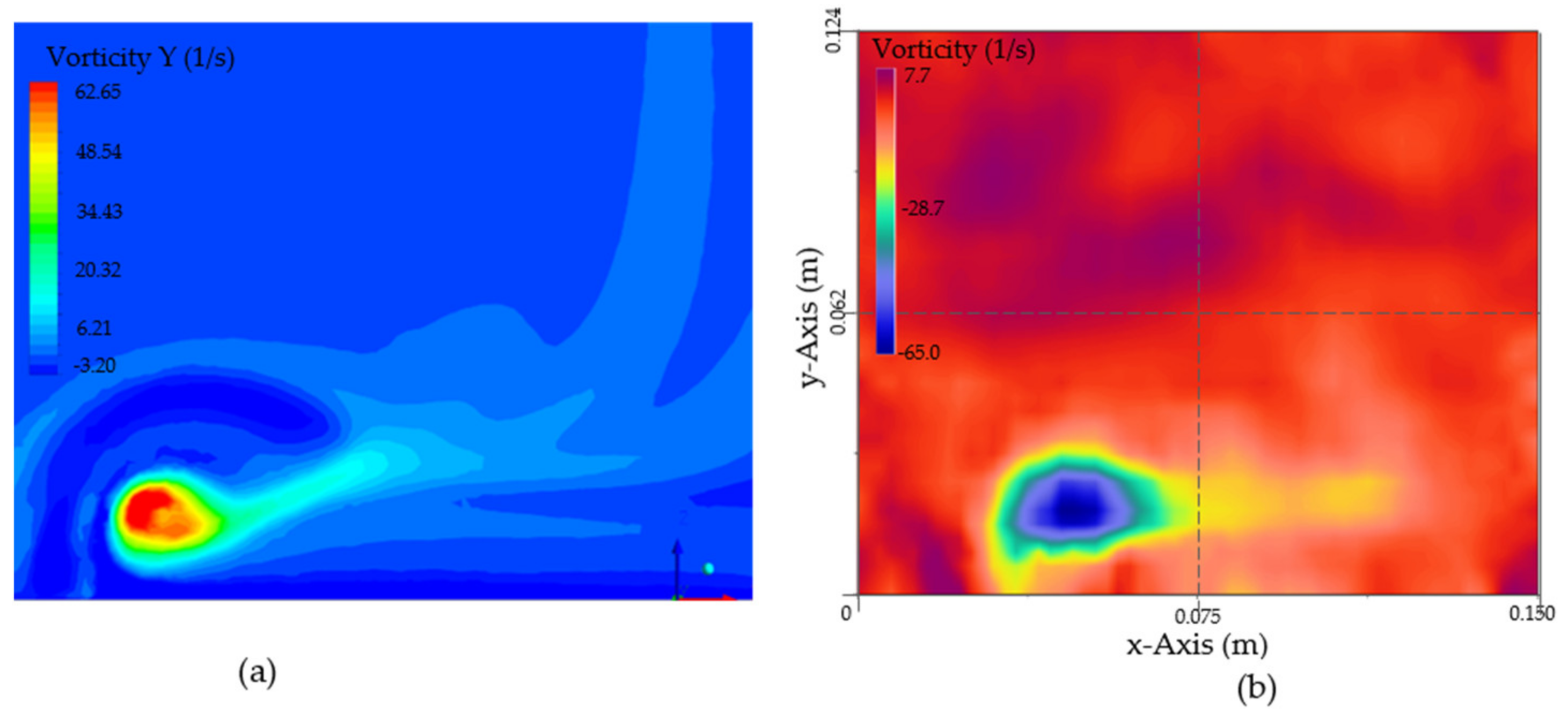
The steady-state analysis considers the flow pattern as a “converged stable” state and shows an overall average single result. Therefore, as shown in
Figure 8, the vorticity contour of steady-state CFD was similar to the time-averaged PIV post-processed results. In CFD results, the maximum vorticity was measured around the positive y-axis and denoted in red color. However, in PIV results, vorticity was measured around the negative y-axis. Hence the maximum vorticity was identified as the highest negative value denoted in blue color. Here the maximum vorticities at the vortex core are recorded as 62.65 (1/s) and 65 (1/s) in steady-state CFD and time-averaged PIV results, respectively.
In the PIV post-processed results, the position of the subsurface vortices of Type 2 moves 0.03 m in the x-axis direction, where the RANS (SST turbulence) simulation shows similar behavior. Furthermore, the maximum vorticity value at the Type 2 subsurface vortex core is almost similar to the RANS simulation (96.88 (1/s)), with the PIV results (103 (1/s)), as in
Figure 9a,b. However, in the LES simulation, the maximum vorticity was quite high (164.76 (1/s)) compared with the PIV results, as shown in
Figure 9c. Since the same mesh was used in RANS and LES models, the mesh resolution was insufficient in the LES simulation to capture the actual magnitude of vorticity at the side wall. Aljaž Škerlavaj et al. claim the y+ value is in the range of 10–100 at the floor of the vortex core when simulating the pump sump models in LES [
28]. However, the 8.5 y+ value in this study was insufficient to capture the accurate vorticity in Type 2 subsurface vortices at the left wall. Therefore, the mesh should be finer than the current mesh to simulate the LES model having accurate analysis of subsurface vortices. Thus, LES simulation with finer mesh consumes more time to solve, requiring high computational power and storage.
The PIV results for subsurface vortices of Type 2 were analyzed with the transient RANS simulations combined with the SST turbulence model. Dye test visualization and post-process PIV data were used to determine the appearance of Type 2 subsurface vortices. A 60.2 (1/s) average vorticity value was recognized as the reference level to form the Type 2 subsurface vortices, as described in
Section 3. Therefore, the 60.2 (1/s) vorticity line was used as the reference level in both PIV and CFD vorticity analyses.
Figure 10 illustrates the vorticity variation in the vortex core for a single cycle in the post-processed PIV and CFD results. Here, one cycle of Type 2 subsurface vortex phenomena (period of 2.56 s) was divided into a 100-time step. The average cycle value of vorticity in the PIV results was calculated as 65.68 (1/s). The trend of the vorticity of PIV and the CFD results is similar in the presence of the Type 2 subsurface vortex. The maximum vorticity of the Type 2 subsurface vortex was 107.9 (1/s) in the PIV results, whereas 104.9 (1/s) was recorded in CFD results. However, the average vorticity values of Type 2 subsurface vortices are similar in the PIV and CFD results recording 84.63 (1/s) and 85.15 (1/s), respectively. In this case, the error between the PIV and the CFD is 0.62% marking a reasonable agreement.
The vorticity variation in the PIV results is spread due to the limitations of PIV techniques. Since this is a 2D PIV system, it could not provide information on the axial structure of the vortex, even though there were many particles. Furthermore, the grid size of PIV post-process was selected depending on the number of particles in the capture plane [
14]. In addition, the optimal frame per second settings was selected in the high-speed camera to illuminate the particles clearly. The vorticity variation in the CFD results is smoother than that observed in the PIV results due to the fine mesh region where the Type 2 subsurface vortices were formed.
6. Conclusions
This study mainly focuses on analyzing the Type 2 subsurface vortex in the PIV sump test and CFD simulation since the ANSI/HI 9.8 (2018) standard claims avoidance of Type 2 and 3 subsurface vortices in pump sump design. RANS steady-state (SST), RANS transient (SST), and LES transient analyses were considered in the CFD study, whereas RANS transient analysis shows a good agreement with the PIV test results over the other CFD models. RANS steady-state simulations were initially carried out to observe the basic characteristics of Type 2 subsurface vortices, especially comparing the average vorticity magnitude with PIV time-averaged results. Even though the RANS steady-state results are similar to the time-averaged PIV data, it does not imply the dynamic behavior of the Type 2 subsurface vortices in the time frame. The LES transient behavior of Type 2 subsurface vortices differs from the PIV results, especially the vorticity magnitude at the vortex core since the LES model required a lower y+ value despite the current value being 8.5. Therefore, the RANS transient (SST) simulation results were compared with the PIV post-process results in the form of the vorticity of the subsurface vortex core of Type 2.
The dye test was used to determine the reference level of the vorticity when Type 2 subsurface vortices are formed. The periodic behavior of the Type 2 subsurface vortex was used to map the dye test results with the PIV post-processed vorticity values. 60.2 (1/s) vorticity was identified as the reference level to form the Type 2 subsurface vortices. The average vorticities of the Type 2 subsurface vortex were recorded as 84.63 (1/s) and 85.15 (1/s) in PIV and CFD, respectively, showing good agreement. The vorticity variation spreads in the PIV results in the presence of the Type 2 subsurface vortex because of the limitation of the PIV techniques. However, the CFD vorticity variation was smooth in the RANS transient simulation due to the finer mesh in the considered region.
This study concluded by calming the vorticity value of the Type 2 subsurface vortices, which is a criterion to determine the suitability of pump sump design by comparing the model test PIV with the CFD simulation results.


 ,
, 


