Method for Determining Sensor Location for Automated Shading Control in Office Building

Abstract

Shading facilities are important technology to enable the adjustment of the indoor light and heat environment, and the control logic of the technology relies on data collected by sensors. The sensor position is generally arranged on the work surface, which is only suitable for single rooms with fixed locations. For open-plan offices or other large offices, more study of detailed designs for the sensor position is required. Therefore, various sensor locations for different spaces will be investigated. Based on existing research, the UDI_{2000 lux} [50%] and UDI_{450–2000 lux} [50%] are the key indices for measuring sensor location. The Entropy Weight method is used to determine the weight of each index, and the ideal point method (TOPSIS method) is used to select the best sensor location. Based on the results, recommendations are provided for different space scales, window-to-wall ratios, and building orientations of offices for shading control sensor location.

1. Introduction

Shading technology in buildings has been widely applied as an important measure to adjust solar irradiance. The main purpose of blinds is to provide shade from excess solar radiation and they can also effectively reduce the air-conditioning load during the cooling season [1]; however, most designs and practical applications are based on empirical or rough adjustments. With an increasing need to improve indoor working environments, the requirements for shading are no longer satisfied by basic physical performance, and occupants’ comfort and satisfaction has attracted more attention [2]. The design of fixed shading and its need for manual adjustment has been increasingly unable to meet people’s requirements. Existing automatic control logic includes a cut-off angle control, real-time indoor environment parameters, and a control method to reproduce the occupants’ habits [3]. The cut-off angle control method is common, but the adjustment is mainly based on the outdoor solar irradiance, and glare cannot be effectively avoided [4]. The method for reproducing occupants’ habits can adjust the shading according to the occupants’ preference and habits [5]. However, occupant behavior is not entirely focused on building–energy conservation and indoor environment adjustment. A control method based on real-time indoor environment parameters has been developed; however, it is difficult to determine the best sensor position for shading control in smart buildings.

The positioning of sensors for shading control is important; they are generally placed above the work surface, which is suitable for single rooms with fixed locations. However, it is more difficult in open-plan offices or other large offices, and a more detailed design for the sensor position is needed in these cases. If the sensors are set above the work surface, more sensors are required. Therefore, this research proposes a method for selecting the sensor position for automated shading control. The improved UDI index is selected as the key parameter for sensor location selection. The Entropy Weight method is used to determine the weight of each parameter, and the ideal point method (TOPSIS method) is used to select the satisfactory sensor location.

2. Automated Shading Control Related Works

2.1. Literature Review

The existing shading control method uses physical environment parameters, which often include work surface illuminance, but illuminance sensors cannot be installed on desktops. Some researchers have focused on comprehensive shading control measurements by combining the internal solar radiation intensity, external walls with indoor light environment parameters, and indoor temperature [6], or by composite light environment indices such as glare indices (DGI, PGSV [7]) or software simulated indices (vertical illuminance at the human eye (E_v) [8], etc.).

Table 1. Sensor location information of domestic and international automatic shading control logic in recent years.

Researchers	Time	Parameters	Sensor Location
C. Goovaerts [9]	2017	Daylight Glare Probability (DGP)	2 m from window, 1.4 m high
H. Burak Gunay [10]	2016	Illuminance of ceiling	3 m from window, above working plane
Toshie Iwata [8]	2016	Predicted Glare Sensation Vote (PGSV)	2.5 m from window, 1.2 m high
Martin Thalfeldt [11]	2014	Indoor temperature Illuminance of working plane	Ceiling above seat
Ying-Chieh Chan [4]	2013	Under direct solar radiation or not DGP	2 m from window, 1.15 m high
Myung Hwan Oh [12]	2012	Daylight Glare Index (DGI) Indoor temperature	2 m from window, 1.65 m high
So Young Koo [13]	2010	Under direct solar radiation or not	Assigned seat level
Jia Hu [14]	2010	Illuminance of working plane	0.75 m and 2.75 m from window, 0.75 m high

summarizes the physical environment control parameters and the corresponding sensor location for automatic shading control methods, as reported in the literature in recent years.

All the shading control methods are based on sensor data, which are generally applicable to single rooms with fixed locations. For open-plan offices or other large spaces, these control methods are not applicable, and a detailed design for the sensor location is required.

2.2. Key Parameters for Shading Control

The regulatory standard for lighting in the indoor environment is based on a principle of making full use of natural lighting. The regulation of the light environment in office buildings should not only consider the full utilization of natural lighting, but also include the control of glare. Therefore, shade control logic must consider both the abundance of natural lighting and the glare index.

2.2.1. The Glare Metrics

Glare is a kind of visual discomfort, and it may be accompanied by short-term visual disability [15]. Glare is experienced when there is a bright object or a strong contrast between the object and the background. According to the source of glare, it can be divided into artificial light glare and daylight glare. For artificial light sources, the Glare Index (GI), VCP (Visual Comfort Probability), brightness limit curve, and UGR (Unified Glare Index) are used to describe the glare metrics. These indices are calculated by assuming a uniform brightness for the background, without considering the global brightness of the scene. Therefore, they cannot describe daylight glare [16,17].

At present, the commonly used daylight glare indices are Daylight Glare Index (DGI) [18] and Daylight Glare Probability (DGP) [19]. DGI was proposed by Hopkinson in 1972 to predict the glare level under large-area light sources. The hypothetical premise of the index is that when a person looks from a room through a window to the exterior, the brightness of the sky, the ground, and the building in the field of view are all consistent. Since an equivalent uniform artificial light source is used as a substitute for the window during the experiment, it was found that the determined DGI is quite different from the actual situation in the application.

In response to the problem of DGI, Wienold proposed a new daylight glare system—the Daylight Glare Probability (DGP) [20]. In a real sky environment, many experiments are carried out in a laboratory room under given conditions. A digital camera is used to record the brightness distribution in the field of vision of indoor personnel, and Evalgare software is used to analyze and process the data to determine the glare-producing area, forming a glare prediction system. A large number of studies have shown that DGP has strong accuracy and consistency [21], and it is widely used by scholars. Although the index has high accuracy, the calculation process is very time-consuming, which is only suitable for specific requirements with high accuracy. Point calculations are not suitable for large planes in full space.

Both DGI and DGP indices are directly related to glare comfort. The two indices are accurate, but the related calculation is complicated. Therefore, Azza Nabil proposed the UDI (Useful Daylight Illuminance) index system to describe the natural lighting effect of the space to solve this problem [22]. This index is calculated based on a standard year-round sky model, where different daylighting effects are divided into intervals, as shown in

Table 2. The relationship between daylighting effect and illuminance interval divided by UDI index.

UDI	Light Environment
UDI < 100 lux	Insufficient lighting, dim vision
100 lux ≤ UDI < 2000 lux	Effective lighting
UDI ≥ 2000 lux	Excessive lighting, visual discomfort

. After comparing various thresholds and crowd acceptance, Azza Nabil proposed the ${\mathrm{UDI}}_{2000 \mathrm{lux}}$ as an index to describe the critical line of spatial glare. When the UDI is greater than 2000 lux [23], the point (the space) is more likely to contain glare, causing visual discomfort. Since the UDI was proposed, it has been widely recognized and used. Although the index is not as accurate as DGP, its calculation is convenient and fast, and it is suitable for large-space calculations that do not require high precision.

According to the regulations of the UDI index system, when it is necessary to simulate and evaluate the indoor lighting situation (glare situation) for a large space, the $UD{I}_{2000\mathrm{lux}}$ [50%] index should be used to evaluate the glare situation in the whole room. The $UD{I}_{2000\mathrm{lux}} \left[50\%\right]$ is defined as the proportion of an indoor table surface that has illuminance greater than 2000 lux for more than half a year for the total area of the work surface.

2.2.2. Daylighting Design

The daylight factor and work surface illuminance are proposed in the Standard for Daylighting Design of Buildings in China [24].

The daylight factor evaluates whether the layout and structural design of windows and sunshades related to daylighting in the room is conducive to the use of natural lighting. This index cannot be used to evaluate the real indoor lighting conditions under a variety of weather conditions, especially under sunny conditions where direct solar radiation cannot be ignored. In this research, the control of glare will involve a direct sunlight scenario.

In the Standard for Daylighting Design of Buildings, the work surface illuminance index and the standard value of natural illuminance are used to evaluate the indoor natural lighting effect. Compared with the lighting factor, work surface illuminance can better describe the specific daylighting effect, focusing on the indoor lighting environment rather than the layout design of the building lighting facilities. For different space types, the standard provides a height definition for the sitting position and a corresponding work surface illumination threshold. However, the standard only provides a lower limit for the threshold. According to recent literature reviews, an important scenario of an uncomfortable light environment in office spaces is the glare phenomenon caused by excessive lighting. Therefore, it is not accurate to only set the lower threshold of work surface illumination. At the same time, according to the requirements of the daylighting measurements method [25], indoor illuminance is measured from 10 a.m. to 2 p.m. on a certain day, and the test is carried out under relatively stable illuminance conditions. Therefore, this index only reflects the light environment at the time of the test and is unable to reflect the quality of the indoor light environment throughout the year.

The UDI mentioned above uses hourly data for the weather conditions in the standard meteorological documents of various localities as the environmental boundary conditions, and the annual hourly illuminance value is calculated at any point in the building space. Therefore, compared with work surface illuminance, it is more comprehensive in terms of time and can better characterize the advantages and disadvantages of the indoor light environment of the building.

The UDI index commonly used is from 100 lux to 2000 lux. The illuminance interval has been determined to improve the universality of the index based on research results related to visual comfort around the world. In the Standard for Daylighting Design of Buildings, according to actual conditions in China and the light adaptability of personnel, the lower limit of the targeted natural illuminance standard value is defined. For office spaces the standard value is set at 450 lux.

Therefore, the internationally accepted UDI index description method and the existing Chinese lighting standards have been combined in this study. Herein, it is proposed to divide the indoor daylighting from 450 lux–2000 lux, and the effectiveness of the whole room lighting would be calculated. $UD{I}_{450-2000\mathrm{lux}} \left[50\%\right]$ is defined as the proportion of the indoor workplane with an illuminance between 450 lux and 2000 lux for more than half a year for the total area of the work surface. This $UD{I}_{450-2000\mathrm{lux}} \left[50\%\right]$ index is better at describing indoor lighting, and it is proposed that it be used to describe the lighting abundance in the whole room.

3. Method of Sensor Location for Automated Shading Control

The sensor location needs to consider both the glare index and the effective daylighting. This section will state the principles, steps, and specific method for determining the best sensor location.

3.1. The Principles for Sensor Location

According to the existing research foundation of shading control in buildings, the following three principles of sensor location for shading adjustment have been determined.

(1)

For the selection of the sensor position in the shading control logic, the glare index, effective daylighting, and the lighting effect on the whole room for the different control objects should be considered.

(2)

The $UD{I}_{2000\mathrm{lux}}$ [50%] and $UD{I}_{450-2000\mathrm{lux}}$ [50%] index should be used to compare and analyze a whole year, working hours should be selected for calculation and processing, and consideration should be given to the changes of the four seasons as well as the shading effect during the work day so that the results are representative.

(3)

Only one sensor position should be used to control the shading for a small room, and the glare index calculated from this sensor should trigger the shading adjustment. The shading control logic should be simple, the project investment should be low, and the practical application should be simple.

3.2. The Steps for Sensor Location

Based on the principles above, a method for determining the sensor position for indoor shading control is divided into the following steps:

(1)

Divide the work surface into grids, to ensure all sensor positions in the room are considered.

(2)

Substitute all the sensor positions into the shading control logic. Obtain the $UD{I}_{450-2000\mathrm{lux}}$ [50%] and $UD{I}_{2000\mathrm{lux}}$ [50%] index values corresponding to each shading control position by indoor light environment numerical simulation methods.

(3)

Obtain the optimal sensor position for shading control using a suitable multi-attributes decision-making method to prioritize the schemes. The index is called attributes.

The next section will specifically introduce the multi-attributes decision-making method used in this study.

3.3. The Multi-Attributes Decision-Making Method

Multi-Attributes Decision-Making is the theoretical method of scientific and reasonable selection for multiple contradictory objectives and the related decision-making. The analytic hierarchy process (AHP), the ideal point method (TOPSIS method), and simple linear weighting method are suitable for multi-objective decision-making with limited alternatives. The sensor location determining for shading control is a limited multi-attribute decision. Through comparative analysis of the applicability, advantages, and disadvantages of each method, this study adopted TOPSIS method to determine the sensor position.

The principle of the TOPSIS method is to detect the distance of the evaluation object from the optimal solution and the worst solution. This method fully considers the limitations of limited schemes and is suitable for multi-attribute decision-making problems with a simple attribute structure, limited schemes, and clear goals [26].

The TOPSIS method for program selecting can be divided into four steps as follows.

(1)

Construct a normalized matrix

$$\mathrm{V}=\left\{\begin{array}{c}\begin{array}{ccc}{\mathsf{\omega }}_1{\mathrm{y}}_{11}& {\mathsf{\omega }}_2{\mathrm{y}}_{12}& \dots \end{array}\\ \begin{array}{ccc}{\mathsf{\omega }}_1{\mathrm{y}}_{21}& {\mathsf{\omega }}_2{\mathrm{y}}_{22}& \dots \end{array}\\ ⋮\end{array}\right\}=\left\{\begin{array}{c}\begin{array}{ccc}{\mathrm{P}}_{11}& {\mathrm{P}}_{12}& \dots \end{array}\\ \begin{array}{ccc}{\mathrm{P}}_{21}& {\mathrm{P}}_{22}& \dots \end{array}\\ ⋮\end{array}\right\}$$

(1)

where $\mathsf{\omega }$ is the weight of each attribute, and ${\mathrm{y}}_{\mathrm{ij}}$ is the j-th attribute value of the i-th scheme after normalization of the same trend.

(2)

Determine the positive ideal point ${\mathrm{P}}^{+}$ and the negative ideal point ${\mathrm{P}}^{-}$

$${\mathrm{P}}^{+}=\left\{\begin{array}{c}{\mathrm{maxP}}_{\mathrm{ij}},\mathrm{j} \mathrm{is} \mathrm{the} \mathrm{positive} \mathrm{index}\\ {\mathrm{minP}}_{\mathrm{ij}},\mathrm{j} \mathrm{is} \mathrm{the} \mathrm{negitive} \mathrm{index}\end{array}\right\}$$

(2)

$${\mathrm{P}}^{-}=\left\{\begin{array}{c}{\mathrm{minP}}_{\mathrm{ij}},\mathrm{j} \mathrm{is} \mathrm{the} \mathrm{positive} \mathrm{index}\\ {\mathrm{maxP}}_{\mathrm{ij}},\mathrm{j} \mathrm{is} \mathrm{the} \mathrm{negitive} \mathrm{index}\end{array}\right\}$$

(3)

(3)

Calculate the distance between each solution and the positive ideal point or the negative ideal point.

$${\mathrm{d}}_{\mathrm{i}}^{+}=\sqrt{{{\displaystyle \sum }}_{\mathrm{j}=1}^{\mathrm{m}}{\left({\mathrm{P}}_{\mathrm{ij}}-{\mathrm{P}}^{+}\right)}^2}$$

(4)

$${\mathrm{d}}_{\mathrm{i}}^{-}=\sqrt{{{\displaystyle \sum }}_{\mathrm{j}=1}^{\mathrm{m}}{\left({\mathrm{P}}_{\mathrm{ij}}-{\mathrm{P}}^{-}\right)}^2}$$

(5)

where j is the attribute, and there are m attributes in total.

(4)

Calculate the relative proximity between each solution and the ideal solution

The relative proximity:

$${\mathrm{C}}_{\mathrm{i}}=\frac{{\mathrm{d}}_{\mathrm{i}}^{-}}{{\mathrm{d}}_{\mathrm{i}}^{-}+{\mathrm{d}}_{\mathrm{i}}^{+}}$$

(6)

Arrange the schemes in descending order of ${\mathrm{C}}_{\mathrm{i}}$.

3.4. Determining the Attributes’ Weight

The subjective weighting method, expert rating method, analytic hierarchy process weighting method, entropy weight method, etc., are used to determine the weight of the attribute. The subjective weighting method, expert rating method, and analytic hierarchy process all have a subjective component for determining the attribute weights. In this study, the shading control logic proposed is to serve non-designated groups, and the balance between lighting and glare control for the light environment for the whole space is more objectively considered. Therefore, a more objective Entropy Weight method is selected to determine the weight of the two attributes.

The Entropy Weight method is an objective weighting method that assigns weight to attributes based on the information entropy of the attributes. The greater the difference between the results of a certain attribute in each scheme, the greater the information entropy. Thus, the greater the information value of the attribute, the greater the weight that is given to the attribute. This method determines the weight of each attribute based on the characteristics of the data themselves, and it is relatively objective.

Using the Entropy method to calculate the attribute weights, it is divided into three steps as follows.

(1)

Attribute index normalization

Choose the deviation standardization method to normalize the index as follows.

Standardization of positive index:

$${\mathrm{x}}_{\mathrm{ij}}=\frac{{\mathrm{x}}_{\mathrm{ij}}-\min \left\{{\mathrm{x}}_{1\mathrm{j}},{\mathrm{x}}_{2\mathrm{j}},{\mathrm{x}}_{3\mathrm{j}}\dots {\mathrm{x}}_{\mathrm{nj}}\right\}}{\max \left\{{\mathrm{x}}_{1\mathrm{j}},{\mathrm{x}}_{2\mathrm{j}},{\mathrm{x}}_{3\mathrm{j}}\dots {\mathrm{x}}_{\mathrm{nj}}\right\}-\min \left\{{\mathrm{x}}_{1\mathrm{j}},{\mathrm{x}}_{2\mathrm{j}},{\mathrm{x}}_{3\mathrm{j}}\dots {\mathrm{x}}_{\mathrm{nj}}\right\}}$$

(7)

Standardization of negative index:

$${\mathrm{x}}_{\mathrm{ij}}=\frac{\max \left\{{\mathrm{x}}_{1\mathrm{j}},{\mathrm{x}}_{2\mathrm{j}},{\mathrm{x}}_{3\mathrm{j}}\dots {\mathrm{x}}_{\mathrm{nj}}\right\}-{\mathrm{x}}_{\mathrm{ij}}}{\max \left\{{\mathrm{x}}_{1\mathrm{j}},{\mathrm{x}}_{2\mathrm{j}},{\mathrm{x}}_{3\mathrm{j}}\dots {\mathrm{x}}_{\mathrm{nj}}\right\}-\min \left\{{\mathrm{x}}_{1\mathrm{j}},{\mathrm{x}}_{2\mathrm{j}},{\mathrm{x}}_{3\mathrm{j}}\dots {\mathrm{x}}_{\mathrm{nj}}\right\}}$$

(8)

where n is the number of plans sets, i refers to the i-th plan, and j refers to the j-th index.

(2)

Calculate attribute information entropy

According to the theory of information entropy, the greater the uncertainty, the greater the entropy, and the greater the amount of information contained. In the entropy weight method, the degree of the dispersion index (entropy redundancy) is judged by calculating the entropy value. When the redundancy of the entropy for a certain attribute is greater, the information value of the attribute is higher, and the greater value is given to the attribute.

The equation for solving information entropy redundancy is as follows:

$${\mathrm{d}}_{\mathrm{j}}=1-{\mathrm{e}}_{\mathrm{j}}$$

(9)

$${\mathrm{e}}_{\mathrm{j}}=-\frac{1}{\ln \left(\mathrm{n}\right)}{{\displaystyle \sum }}_{\mathrm{i}=1}^{\mathrm{n}}{\mathrm{p}}_{\mathrm{ij}}\ln \left({\mathrm{p}}_{\mathrm{ij}}\right)$$

(10)

where ${\mathrm{p}}_{\mathrm{ij}}$ is the proportion of the sample value in the index under the index. The equation is as follows:

$${\mathrm{p}}_{\mathrm{ij}}=\frac{{\mathrm{x}}_{\mathrm{ij}}}{{{\displaystyle \sum }}_{\mathrm{i}=1}^{\mathrm{n}}{\mathrm{x}}_{\mathrm{ij}}}$$

(11)

(3)

Calculate the weight of the attribute

After obtaining the entropy redundancy of each attribute, the weight of each attribute is obtained by the following equation.

$${\mathrm{W}}_{\mathrm{j}}=\frac{{\mathrm{d}}_{\mathrm{j}}}{{{\displaystyle \sum }}_{\mathrm{j}=1}^{\mathrm{m}}{\mathrm{d}}_{\mathrm{j}}}$$

(12)

In this study, the Entropy Weight and TOPSIS method are used to conduct multi-objective decision-making research on the recommended values for the comprehensive shading control. $UD{I}_{450-2000\mathrm{lux}}$ [50%] is used to describe the lighting abundance in the whole room after shading adjustment, and it is a positive index; $UD{I}_{2000\mathrm{lux}}$ [50%] is used to evaluate the glare in the whole room after shading adjustment, and it is a negative index.

4. Analysis and Discussion

This section will discuss the optimal sensor position for shading control in a small office space and an open-plan office space based on the method above. The optimal sensor location is researched for the different window-to-wall ratios and building orientations.

4.1. Model Parameters

Three office buildings located in Shanghai are investigated. Building 1 had four floors above the ground, and the overall orientation is due south. Building 2 had six floors above the ground, and the overall orientation is 8° east of south. Building 3 is an office building with five floors above the ground, and the overall orientation is 10° west of south. In the three buildings, there are two types of office spaces. The first type of office space holds more than 50 people, and the office space area is 80–120 square meters. The second type of office space holds less than six people, and the area is about 30 square meters. These two types of office spaces are named “open-plan office room” and “small office room”.

For the two types of office rooms, the corresponding characteristics are shown in

Table 3. Characteristics of the two types of office spaces.

Space Type	Area	Shape Feature	Orientation	Window-to-Wall Ratio
Open-plan office space	80~120 m2	East–west strip	South	0.5~0.7
Small office space	Around 30 m2	North–south strip	South	0.3~0.7
			East	0.4~0.5
			North	0.2~0.3

. The room models are established, and the relevant parameters of the model are shown in

Table 4. Model related parameters.

City	Space Type	Space Size (Width × Depth × Height)/m	Orientation	Window-to-Wall Ratio
Shanghai	Open-plan office space	16 × 8 × 3	South	0.5
			South	0.3/0.5/0.7
	Small office space	4.5 × 7.5 × 3	East	0.4
			North	0.2

.

According to the method described in the previous section, the space plane is divided into grids. The candidate sensor positions are shown in Figure 1 and Figure 2 for the two types of rooms. Each sensor location is named RiEAST/WESTj in the figures, where Ri stands for i meters from the south window. MIDDLE indicates that the sensor is located on the central axis. EAST/WESTj indicates that the sensor is located on the east/west side of the central axis and is j meters away from the central axis.

The Entropy Weight and TOPSIS method are used to determine the sensor location for shading control. The sensor locations will be obtained after the shading control effect is simulated in the DIVA software, and the position data of the shading sensor are standardized by Equations (7) and (8). The attribute information entropy will be calculated used Equations (9)–(11); the weight of $UD{I}_{450-2000\mathrm{lux}}$ [50%] and $UD{\mathrm{I}}_{2000\mathrm{lux}}$ [50%] are obtained by Equation (12). According to the TOPSIS method, the order of each sensor location is obtained by Equations (1)–(6). Based on the methods, the different window-to-wall ratios and building orientations effect on the sensor location of shading control will be researched, and the details are as follows.

4.2. Shading Control Sensor Position in Different Rooms

In order to eliminate the influence of other factors when discussing the impact of space scale, the location and window-to-wall ratio of the model should be the same. In this section, a small office room with a window-to-wall ratio of 0.5 in the south area and an open-plan office room with the same window-to-wall ratio and building orientation are analyzed for comparison.

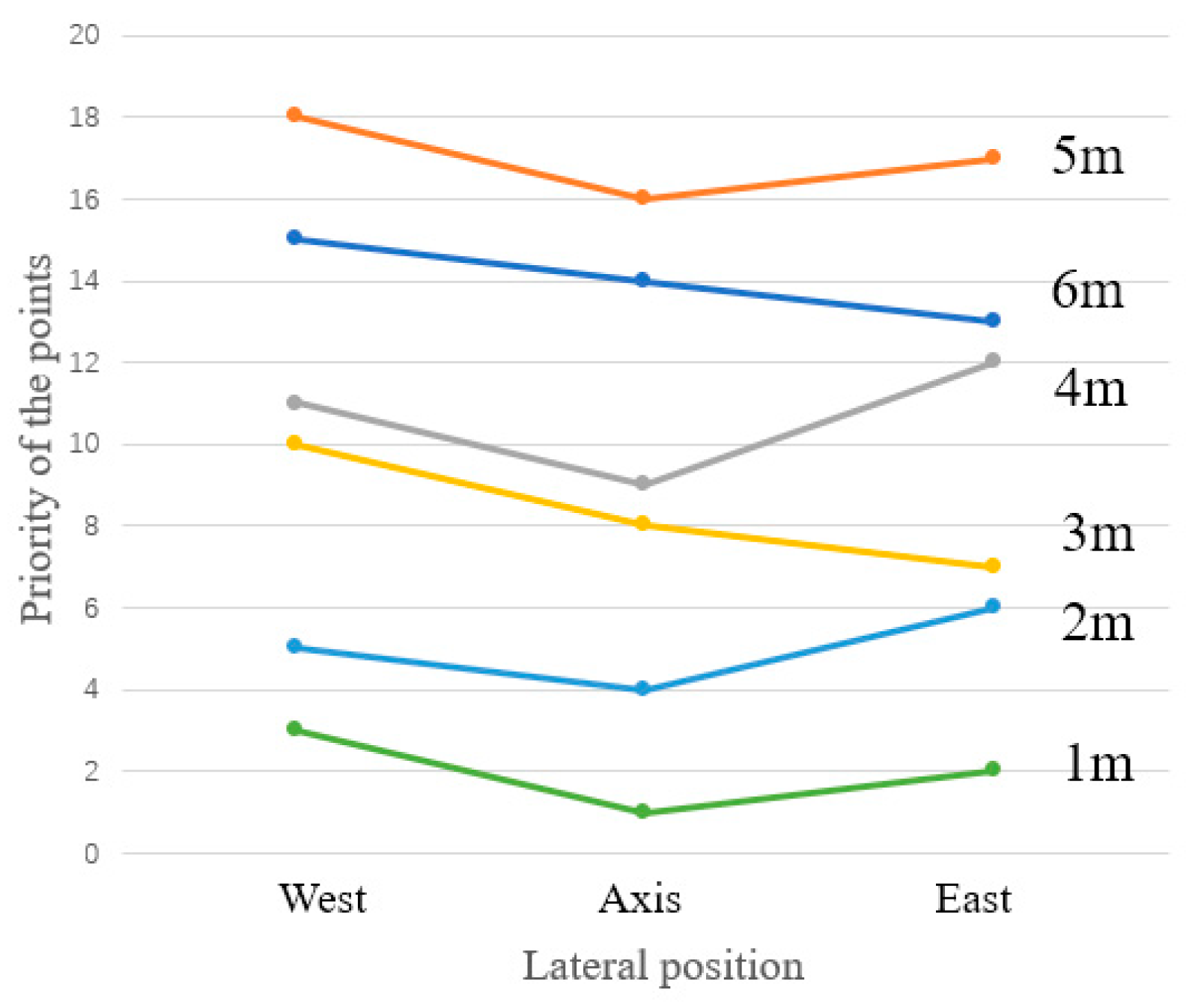
4.2.1. The Characteristics of the Sensor Location in a Small Office Room

The lighting index $UD{I}_{450-2000\mathrm{lux}} \left[50\%\right]$ and glare index $UD{I}_{2000\mathrm{lux}}$ [50%] are used to evaluate the indoor light environment for shading control based on each reference sensor setpoint. According to the light environment requirements, $UD{I}_{450-2000\mathrm{lux}} \left[50\%\right]$ should be larger, and $UD{I}_{2000\mathrm{lux}}$ [50%] should be smaller. The results of all reference sensor locations in the small office room are shown in

Table 5. Adjustment results of all reference sensor locations in the small office room.

Location	$\mathit{U}\mathit{D}{\mathit{I}}_{450-2000\mathbf{lux}} \left[50\mathit{\%}\right]$	$\mathit{U}\mathit{D}{\mathit{I}}_{2000\mathbf{lux}} \left[50\mathit{\%}\right]$
R1-EAST	0.178	0.063
R1-MIDDLE	0.178	0.063
R1-WEST	0.178	0.063
R2-EAST	0.240	0.100
R2-MIDDLE	0.223	0.088
R2-WEST	0.223	0.088
R3-EAST	0.315	0.125
R3-MIDDLE	0.305	0.125
R3-WEST	0.285	0.125
R4-EAST	0.334	0.156
R4-MIDDLE	0.349	0.131
R4-WEST	0.343	0.138
R5-EAST	0.355	0.175
R5-MIDDLE	0.351	0.169
R5-WEST	0.341	0.169
R6-EAST	0.365	0.175
R6-MIDDLE	0.365	0.175
R6-WEST	0.365	0.175

.

According to the Entropy Weight method (by Equations (7)–(12)), the weights of $UD{I}_{450-2000\mathrm{lux}} \left[50\%\right]$ and $UD{I}_{2000\mathrm{lux}}$ [50%] in the small office room are shown in

Table 6. The weights of $UD{I}_{450-2000\mathrm{lux}} \left[50\%\right]$ and 𝑈𝐷𝐼_2000lux [50%] in the small office space.

Index	Weight
𝑈𝐷𝐼450−2000lux [50%]	0.360
$UD{I}_{2000\mathrm{lux}}$ [50%]	0.640

. The weight of glare control is much greater than that of effective daylighting. A change in the sensor location greatly affected the glare but had a relatively small effect on the lighting. According to the TOPSIS method (by Equations (1)–(6)), the order of the priority of each position obtained is shown in Figure 3. The smaller the number in the figure, the higher the priority of the scheme, and the numbers from small to large indicate that the color changes from dark to light.

As shown in Figure 4, the closer the sensor is to the south-facing window, the higher the priority. In the case of the same depth, the sensor location at the central axis is superior to the point position on both sides. Within 5 m of the window, the influence of the axial depth on the sensor location priority is greater than that of transverse distance, and with the change of depth, the priority of the sensor location has an obvious step change. When the axial distance is more than 4 m with increasing depth, the priority of the point position appears to show an inverse phenomenon. This occurs because when the point depth is greater than 5 m, the marginal effect of glare control is rapidly weakened with a further increase in depth, and it is no longer feasible to sacrifice daylighting for glare control.

For the small office room, the influence of glare control on the sensor location is greater than daylighting. It is suitable to arrange the sensor location of shading control near the window, but not 5 m away from the depth.

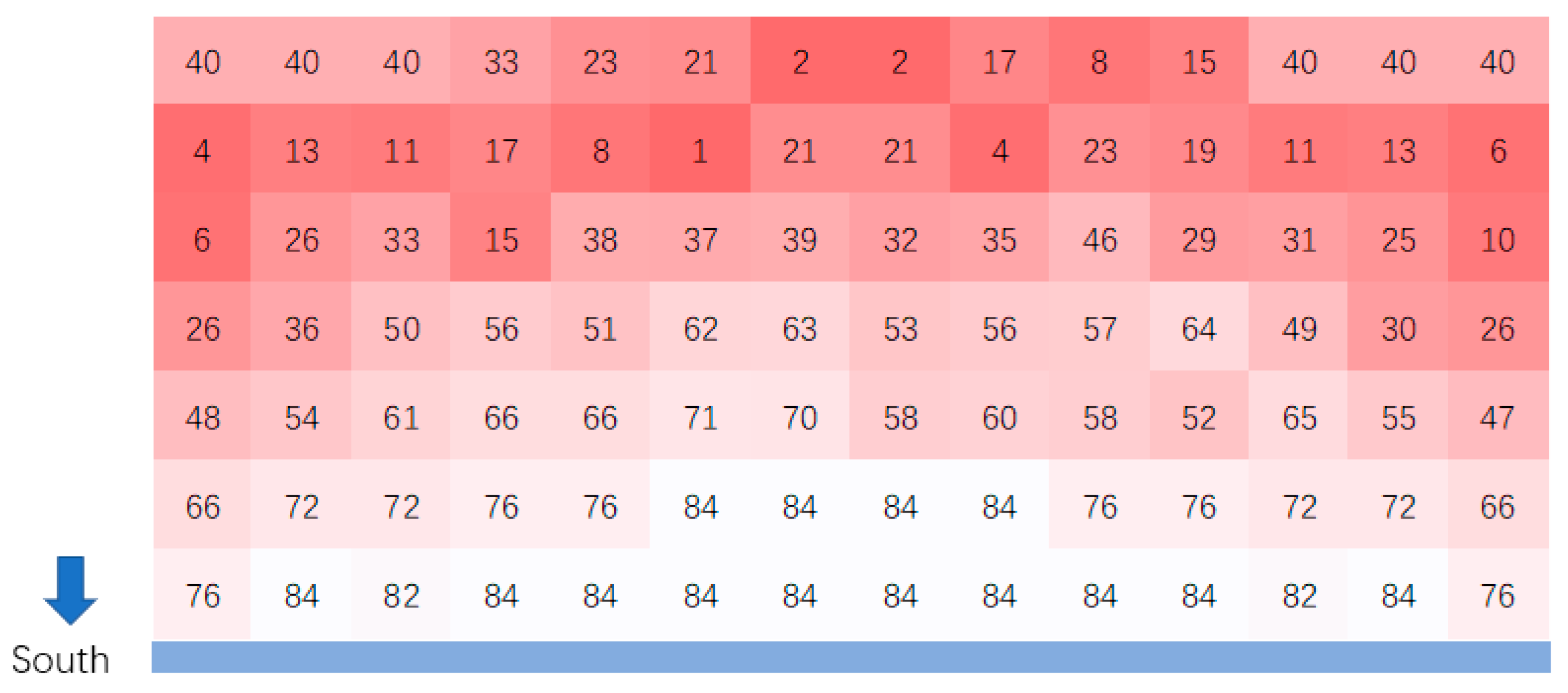
4.2.2. The Characteristics of Sensor Locations in the Open-Plan Office Room

According to the Entropy Weight method (by Equations (7)–(12)), the $UD{I}_{450-2000\mathrm{lux}} \left[50\%\right]$ and $UD{I}_{2000\mathrm{lux}}$ [50%] values of all sensor location in open-plan office room can also be calculated. The weights obtained are shown in

Table 7. The weights of 𝑈𝐷𝐼_{450−2000lux} [50%] and 𝑈𝐷𝐼_2000lux [50%] in the open-plan office room.

Index	Weight
$UD{I}_{450-2000\mathrm{lux}} \left[50\%\right]$	0.726
$UD{I}_{2000\mathrm{lux}}$ [50%]	0.274

.

According to the principle of the Entropy Weight method, the weight of daylighting is greater than glare control for the open-plan office room. This means that the change of sensor location greatly affected daylighting, and the effect on glare control was relatively small. The result is the exact opposite in the small office room. According to the TOPSIS method (by Equations (1)–(6)), the order of merits and demerits of each point obtained is shown in Figure 5. A smaller number indicates a higher priority in the figure. As shown in Figure 5, the best position is in the middle and back of the space.

According to the priority level of each point scheme, the sensor location priority in the space is divided, as shown in Figure 6. The green area is a relatively poor point range, the yellow region is a relatively general point range, and the pink region is a relatively good point range. At the same depth, the closer the sensor locations are to the central axis, the higher the priority, and the best point range is at a depth of 5 to 6 m.

4.3. Shading Control Sensor Position on Different Window-to-Wall Ratios

To evaluate the small office space example, the sensor positions selected for shading control, the influence of different window-to-wall ratios on the attribute weights distribution, and the Equal Priority Domains are investigated.

The simulation calculations are carried out on the sensor position in the small office room using three different window-to-wall ratios. The weights of the daylighting index and glare index according to the three ratios are shown in

Table 8. Weights of $UD{I}_{450-2000\mathrm{lux}} \left[50\%\right]$ and $UD{I}_{2000\mathrm{lux}}$ [50%] under different window-to-wall ratios for the small south-facing office room.

Window-to-Wall Ratio	$\mathit{U}\mathit{D}{\mathit{I}}_{450-2000\mathbf{lux}} \left[50\mathit{\%}\right]$	$\mathit{U}\mathit{D}{\mathit{I}}_{2000\mathbf{lux}} \left[50\mathit{\%}\right]$
0.3	0.188	0.812
0.5	0.360	0.640
0.7	0.549	0.451

(by Equations (7)–(12)). The change in the south-facing window-to-wall ratio (SWWR) caused a relatively large change in the weight of $UD{I}_{450-2000\mathrm{lux}} \left[50\%\right]$ and $UD{I}_{2000\mathrm{lux}}$ [50%]. As the SWWR increased, the weight of $UD{I}_{450-2000\mathrm{lux}} \left[50\%\right]$ increased, and the weight of $UD{I}_{2000\mathrm{lux}}$ [50%] decreased. With an increase in the window-to-wall ratio, the difference of the glare index among the sensor positions in the room became smaller. Until the window-to-wall ratio reached 0.7, the difference in the daylighting index between the schemes was greater than the difference in the glare index. At the same time, the weight of the daylighting index became greater than the weight of the glare index.

The simulation results of an indoor environment under different shading controls in the DIVA software are shown in Figure 7; they are made up of 18 simulation results throughout the year. For every small part, the horizontal axis is month from January to December, and the vertical axis is time from 0:00 to 24:00.

When the window-to-wall ratio in the southern zone is greater than or equal to 0.7, each depth of the room is affected by glare. The glare effect is different for the different ratios of the room width and depth. When the window-to-wall ratio in the southern zone is 0.3 or less, it is affected by glare only within a certain depth. Therefore, when the window-to-wall ratio is less than or equal to 0.3, the glare values monitored throughout the year are quite different among the sensor positions. In summary, the smaller the window-to-wall ratio, the greater the weight of the glare index.

According to the TOPSIS method (by Equations (1)–(6)), the division of the priority domain of the shading control sensor position in the horizontal plane of each space with different window-to-wall ratios is shown in Figure 8. When the SWWR increased, the “recommended area” and the “general area” moved backwards and appeared alternately. This is due to the enclosure structure of the south wall that is formed by connecting a number of vertical strip windows and the wall and is closer to the actual office space in the model. The results showed that the light distribution in the space is divided to a certain extent. When the window-to-wall ratio is relatively small (e.g., 0.3), the recommended shading control sensor locations are within 3 m in depth. When the window-to-wall ratio is relatively large (e.g., 0.7), the shading control sensor position should have been placed at the back of the room, where the area is affected by direct radiation earlier in the day.

4.4. Shading Control Sensor Position on Different Building Orientations

Considering the small office rooms as examples, the recommended areas for the sensor position in a north-facing office room, and in an east-facing office room are discussed. The optional positions in the two types of office rooms are shown in Figure 9. The annual glare levels at each location in the two rooms–which are simulated in DIVA software–are shown in Figure 10 and Figure 11. Figure 10 shows the combined simulation results of 18 sensor locations for shading control. Figure 11 shows the combined simulation results of 21 sensor locations for shading control. For every small part in Figure 10 and Figure 11, the horizontal axis is month from January to December, and the vertical axis is time from 0:00 to 24:00.

As shown in Figure 10, the annual glare level of the north-facing room is relatively weak. The glare only appears within 1 m of the window, and it gradually weakens from summer to winter. This contrasts with the year-round trend of glare in the south-facing room. This is due to the sun’s altitude angle being lower in winter, making it easier for the sunlight to enter the south-facing room. In summer, there is less large-scale glare in the south-facing room due to the angle of the sun’s altitude. For the north-facing room, the glare is only possible when the altitude angle is high.

As shown in Figure 11, the glare level in the east-facing room is greater, and the glare appeared relatively early. When the distance from the window increased, the timepoint for the earliest glare appeared unchanged and the disappearance time gradually advanced. On the central axis of the room, within 1 m from the window, the summer glare disappeared at about 16:00 and the winter glare disappeared at about 14:00. At a distance of 3 m from the window, the year-round glare generally ended around 10:00 a.m. The glare in the north part of the room is greater in winter than in summer. The glare in the southern part of the room is greater in summer than in winter. Otherwise, the severity of the glare in the northern area is higher than the glare level in the southern area. This is because Shanghai’s geographical longitude and latitude leads to a lower solar altitude in winter, which affects the north area of the east-facing room with direct sunlight, while the south area receives less direct solar radiation throughout the year.

The calculated proportions of lighting abundance and the glare indexes for the east- and north-facing rooms (by Equations (7)–(12)) are shown in

Table 9. The weights of $UD{I}_{450-2000\mathrm{lux}} \left[50\%\right]$ and $UD{I}_{2000\mathrm{lux}}$ [50%] in the north- and east-facing rooms.

Orientation	𝑈𝐷𝐼450−2000lux [50%]	𝑈𝐷𝐼2000lux [50%]
East	0.790	0.210
North	0.100	0.900

. The priority domain distribution of the sensor location in the two rooms (by calculating used Equations (1)–(6)) is shown in Figure 12 and Figure 13.

The index weights for each of the room orientations are shown in

Table 10. The weights of $UD{I}_{450-2000\mathrm{lux}} \left[50\%\right]$ and $UD{I}_{2000\mathrm{lux}}$ [50%] in each orientation room.

Orientation	Window-to-Wall Ratio	𝑈𝐷𝐼450−2000lux [50%]	𝑈𝐷𝐼2000lux [50%]
East	0.4	0.790	0.210
North	0.2	0.100	0.900
South	0.3	0.188	0.812
South	0.5	0.360	0.640
South	0.7	0.549	0.451

. The orientation has a great influence on the weight of the lighting index and the glare index. The east-facing room takes daylighting as the main consideration, while the north-facing room is completely opposite. For the south-facing room, changes to the weights of the two indices are affected by the window-to-wall ratio.

5. Conclusions

Currently the problem of visual comfort in offices is more serious than thermal comfort, and the most common reason for manual shading adjustment is the glare, so optimization of the light environment should be included when studying shading control. This research aimed to find a method to determine the best sensor location for shading control. Based on the of literature review, the key parameters for shading control in office buildings are analyzed. When evaluating the effects of indoor light environment regulation on shading control, daylighting adequacy and the suppression of glare should be considered. The $UD{I}_{450-2000\mathrm{lux}} \left[50\%\right]$ index and $UD{I}_{2000\mathrm{lux}}$ [50%] index effectively describe the benefits of shading in terms of full room daylighting and glare control throughout the year.

The final location of the shading control is determined by the Entropy Weight and TOPSIS methods, and the method is applied to the architectural model; the influence of the space scale, window-to-wall ratio, and building orientation on the sensor location for shading control is researched and analyzed. For south-facing offices, the scale of the space has a greater impact on the weighting of daylighting and glare indices. For small office rooms, the recommended sensor positions are at the central axis of the window; while in open-plan office rooms, the recommended sensor positions are at the far window, preferably at a depth of 5–6 m. As the window-to-wall ratio increases, the weight of the daylighting index gradually increases, while the weight of the glare index gradually decreases. In the range of 0.3–0.7 window-to-wall ratio, the weights of the daylighting and glare indices basically change linearly, and the recommended sensor location gradually moves away from the windows and toward to the interior of the room. For different building orientation, the shading control sensor location for north-facing rooms should be located as close as possible to the north window, for east-facing rooms should be located as close as possible to the north wall, and for south-facing rooms will be further influenced by the window-to-wall ratio of the south wall.

The simulation case study was carried out to understand the impact of different spaces, window-to-wall ratios, and building orientations on the sensor location for shading control in Shanghai, and a method to determine the best sensor location for shading control in smart building is explored. More research on cities with different climate characteristics is needed in the future.

References

1. Albert, A.T.; Djamel, O. Shading and day-lighting controls energy savings in offices with fully-Glazed façades in hot climates. Energy Build. 2017, 151, 263–274. [Google Scholar] [CrossRef]
2. Pedro, C.S.; Vítor, L.; Marilyne, A. Influence of shading control patterns on the energy assessment of office spaces. Energy Build. 2012, 50, 35–48. [Google Scholar] [CrossRef] [Green Version]
3. Chaiwiwatworakul, P.; Chirarattananon, S.; Rakkwamsuk, P. Application of automated blind for daylighting in tropical region. Energy Convers. Manag. 2009, 50, 2927–2943. [Google Scholar] [CrossRef]
4. Zhang, S.; Birru, D. An open-loop venetian blind control to avoid direct sunlight and enhance daylight utilization. Sol. Energy 2012, 86, 860–866. [Google Scholar] [CrossRef]
5. Borowczyński, A.; Heim, D.; Szczepańska, R.E. Application of Sky Digital Images for Controlling of Louver System. Energy Procedia 2015, 78, 1769–1774. [Google Scholar] [CrossRef] [Green Version]
6. Chan, Y.-C.; Tzempelikos, A. Efficient venetian blind control strategies considering daylight utilization and glare protection. Sol. Energy 2013, 98, 241–254. [Google Scholar] [CrossRef]
7. Meek, C.; Brennan, M. Automated and Manual Solar Shading and Glare Control: A Design Framework for Meeting Occupant Comfort and Realized Energy Performance. In Proceedings of the 40th ASES National Solar Conference 2011 (SOLAR 2011), Raleigh, NC, USA, 17–20 May 2011. [Google Scholar]
8. Iwata, T.; Taniguchi, T.; Sakuma, R. Automated blind control based on glare prevention with dimmable light in open-plan offices. Build. Environ. 2017, 113, 232–246. [Google Scholar] [CrossRef]
9. Goovaerts, C.; Descamps, F.; Jacobs, V. Shading control strategy to avoid visual discomfort by using a low-cost camera: A field study of two cases. Build. Environ. 2017, 125, 26–38. [Google Scholar] [CrossRef]
10. Gunay, H.B.; O’Brien, W.; Beausoleil-Morrison, I.; Gilani, S. Development and implementation of an adaptive lighting and blinds control algorithm. Build. Environ. 2017, 113, 185–199. [Google Scholar] [CrossRef]
11. Thalfeldt, M.; Kurnitski, J. External shading optimal control macros for 1- and 2-piece automated blinds in European climates. Build. Simul. 2014, 8, 13–25. [Google Scholar] [CrossRef]
12. Oh, M.H.; Lee, K.H.; Yoon, J.H. Automated control strategies of inside slat-type blind considering visual comfort and building energy performance. Energy Build. 2012, 55, 728–737. [Google Scholar] [CrossRef]
13. Koo, S.Y.; Yeo, M.S.; Kim, K.W. Automated blind control to maximize the benefits of daylight in buildings. Build. Environ. 2010, 45, 1508–1520. [Google Scholar] [CrossRef]
14. Hu, J.; Olbina, S. Illuminance-based slat angle selection model for automated control of split blinds. Build. Environ. 2011, 46, 786–796. [Google Scholar] [CrossRef]
15. Yun, G.; Yoon, K.C.; Kim, K.S. The influence of shading control strategies on the visual comfort and energy demand of office buildings. Energy Build. 2014, 84, 70–85. [Google Scholar] [CrossRef]
16. Tyukhova, Y.I. Discomfort Glare from Small, High Luminance Light Sources in Outdoor Nighttime Environments. Ph.D Thesis, University of Nebraska—Lincoln, Lincoln, NE, USA, 2015. [Google Scholar]
17. Atzeri, A.M.; Cappelletti, F.; Gasparella, A. Comparison of different glare indices through metrics for long term and zonal visual comfort assessment, Ratio. WWR 2017, 45, 75. [Google Scholar]
18. Carlucci, S.; Causone, F.; De Rosa, F.; Pagliano, L. A review of indices for assessing visual comfort with a view to their use in optimization processes to support building integrated design. Renew. Sustain. Energy Rev. 2015, 47, 1016–1033. [Google Scholar] [CrossRef] [Green Version]
19. Hopkinson, R. Glare from daylighting in buildings. Appl. Ergon. 1972, 3, 206–215. [Google Scholar] [CrossRef]
20. Wienold, J.; Christoffersen, J. Evaluation methods and development of a new glare prediction model for daylight environments with the use of CCD cameras. Energy Build. 2006, 38, 743–757. [Google Scholar] [CrossRef]
21. Mcneil, A.; Burrell, G. Applicability of DGP and DGI for evaluating glare in a Brightly Daylit Space. In Proceedings of the ASHRAE and IBPSA-USA SimBuild 2016, Building Performance Modeling Conference, Salt Lake City, UT, USA, 8–12 August 2016. [Google Scholar]
22. Nabil, A.; Mardaljevic, J. Useful daylight illuminance: A new paradigm for assessing daylight in buildings. Light. Res. Technol. 2005, 37, 41–57. [Google Scholar] [CrossRef]
23. Nabil, A.; Mardaljevic, J. Useful daylight illuminances: A replacement for daylight factors. Energy Build. 2006, 38, 905–913. [Google Scholar] [CrossRef]
24. GB/T 50033-2013; Standard for Daylighting Design of Buildings. China Architecture and Architecture Press: Beijing, China, 2012.
25. GB/T 5699-2017; Method of Daylighting Measurements. China Architecture and Architecture Press: Beijing, China, 2016.
26. Hwang, C.L.; Yoon, K. Multiple Attribute Decision Making: Methods and Applications; Springer: Berlin/Heidelberg, Germany, 1981. [Google Scholar]
Figure 1. Distribution diagram of alternative sensor locations in the open-plan office space.
Energies 15 04931 g001
Figure 2. Distribution diagram of alternative sensor locations in the small office space.
Energies 15 04931 g002
Figure 3. Prioritization of location in the small office space.
Energies 15 04931 g003
Figure 4. Priorities of each depth of the small office space.
Energies 15 04931 g004
Figure 5. Prioritization of sensor location in the open-plan office space.
Energies 15 04931 g005
Figure 6. The priority domain distribution of sensor location in the open-plan office space.
Energies 15 04931 g006
Figure 7. Annual glare levels at each depth of the room when SWWR = 0.3/0.5/0.7.
Energies 15 04931 g007aEnergies 15 04931 g007b
Figure 8. The priority domain distribution of the indoor sensor position when SWWR is equal to 0.3/0.5/0.7.
Energies 15 04931 g008
Figure 9. The distribution of optional sensor locations in the north-facing room and east-facing room.
Energies 15 04931 g009
Figure 10. Annual glare level at each depth of the north-facing room.
Energies 15 04931 g010
Figure 11. Annual glare level at each depth of the east-facing room.
Energies 15 04931 g011
Figure 12. The priority domain distribution of the sensor locations in the north-facing room.
Energies 15 04931 g012
Figure 13. The priority domain distribution of the sensor locations in the east-facing room.
Energies 15 04931 g013