
False Data Injection Attack Detection in Smart Grid Using Energy Consumption Forecasting


Abstract
:1. Introduction
- proposes a real-time forecasting aided anomaly detection technique to identify a specific type of cyber attack in the SCADA system known as false data injection attack.
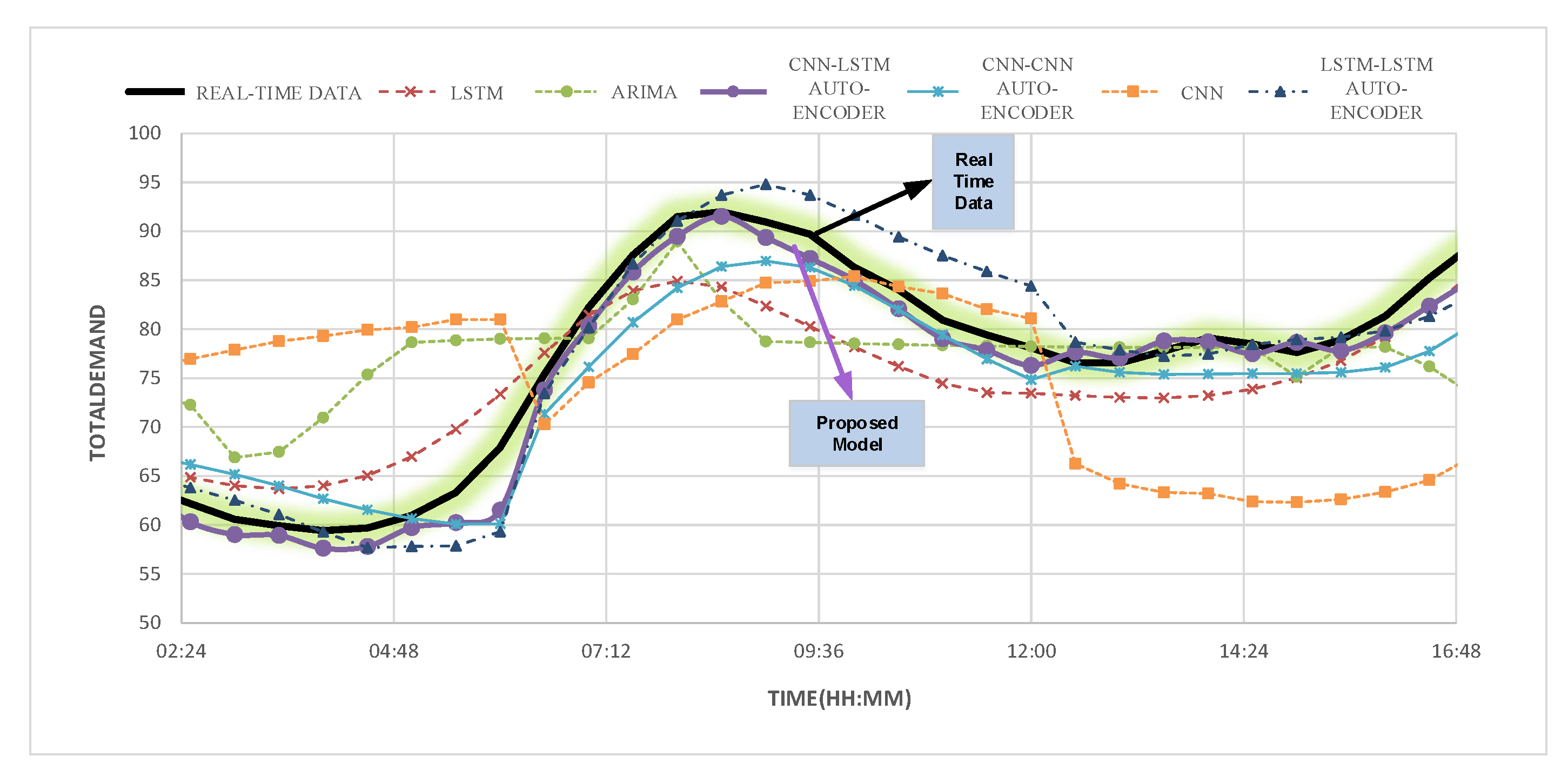
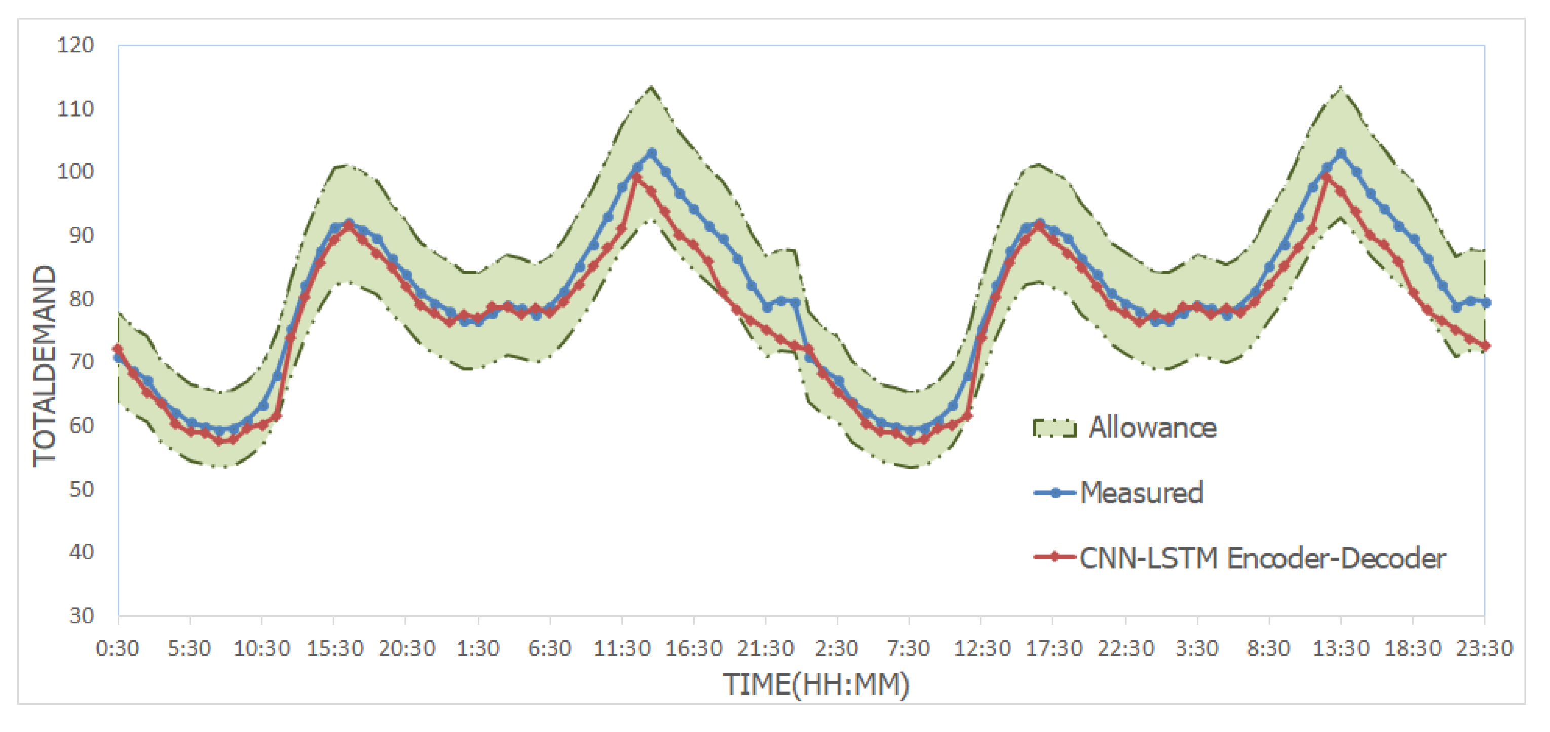
- present CNN-LSTM auto-encoder architecture and determine the existence of the intrusions if the field measurements deviate significantly from the forecasts.
- experiment is conducted on a real-time dataset (Australian Energy Market Operator) that shows a significant gain in performance in comparison to benchmark methods.
2. Related Work
2.1. Forecasting Models
2.2. Forecasting Based Anomaly Detection
3. Proposed Method
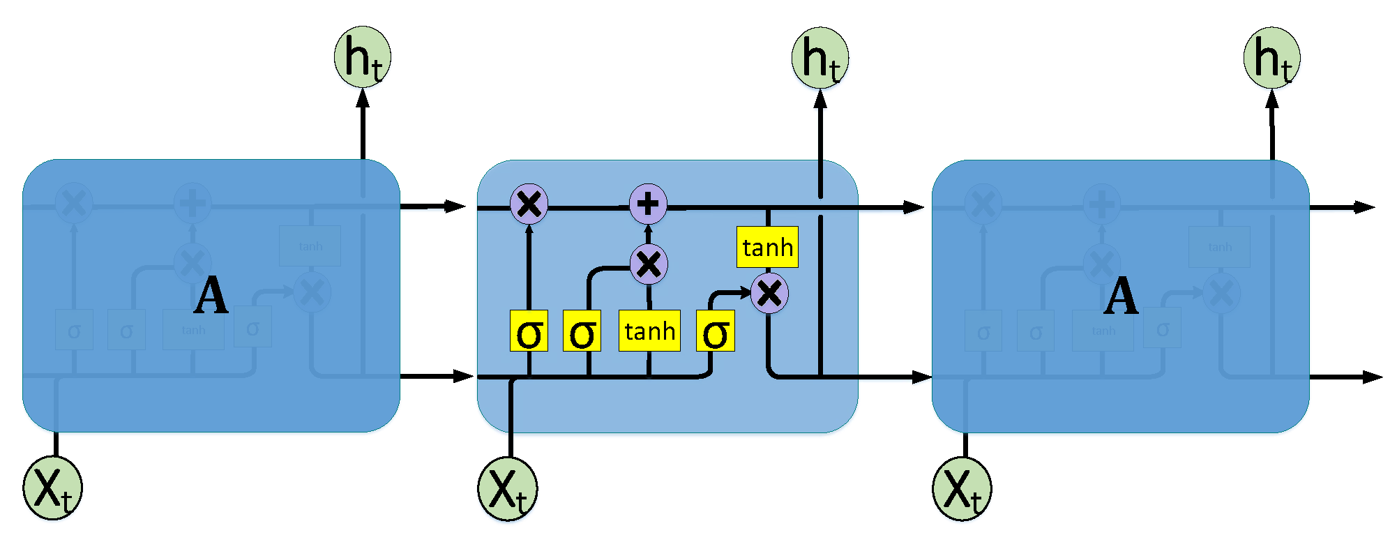
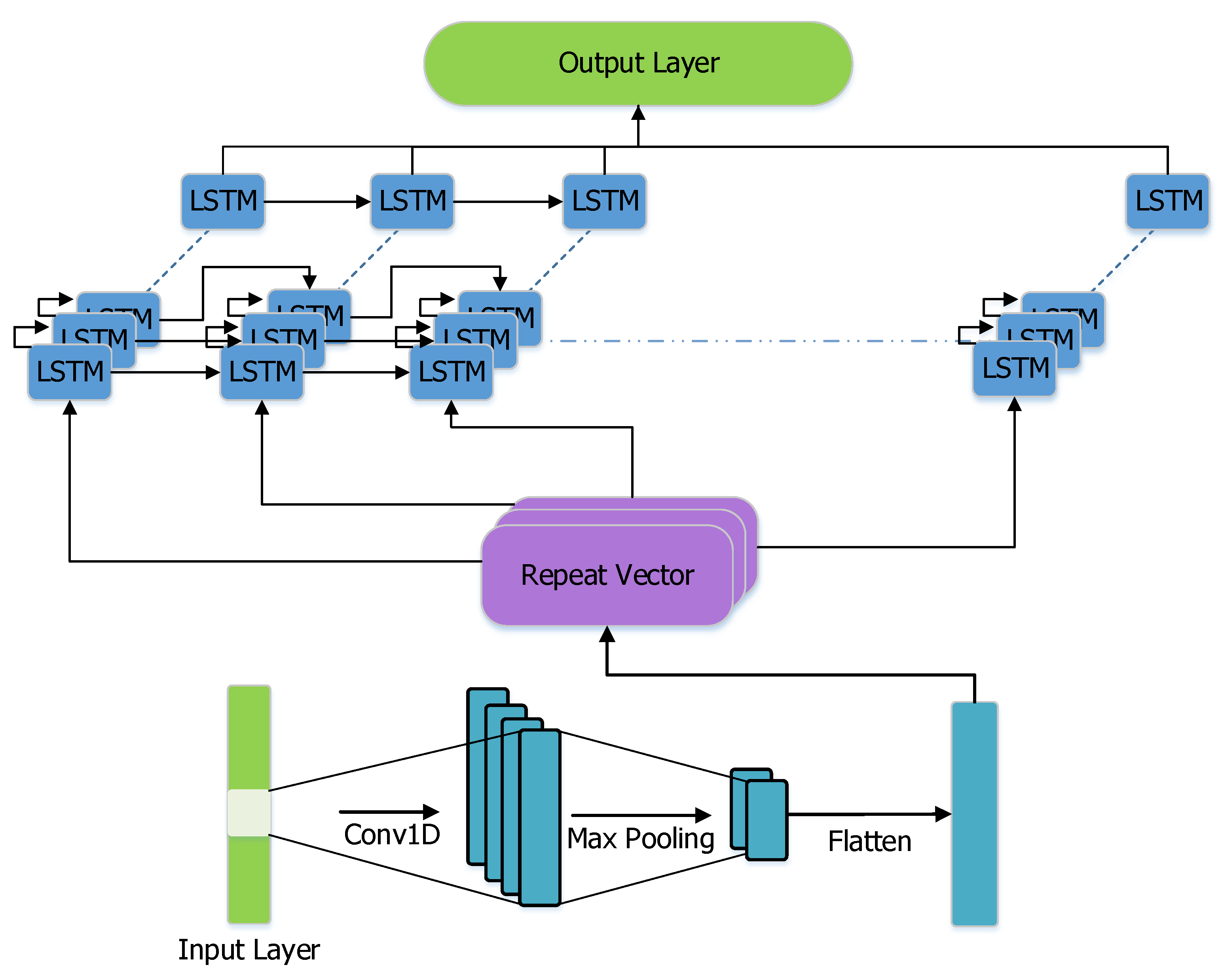
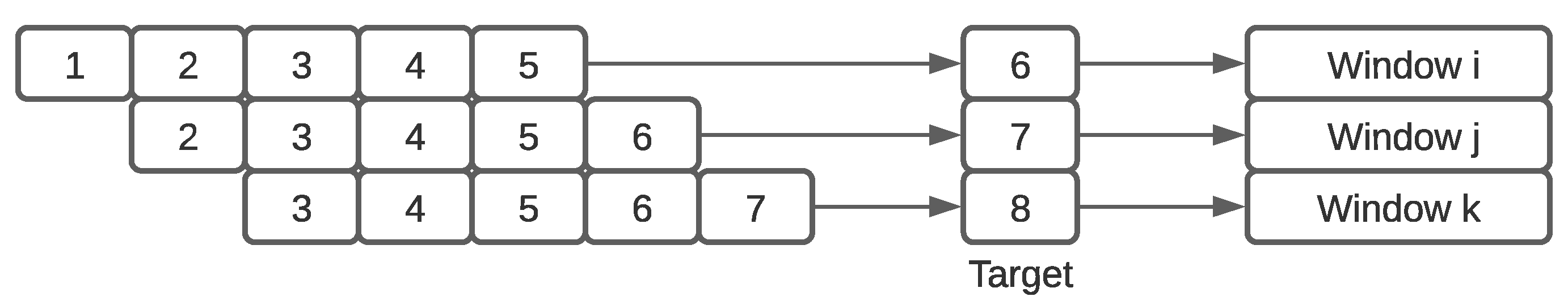
3.1. Energy Consumption Forecasting Using CNN-LSTM Auto-Encoder Sequence to Sequence Architecture
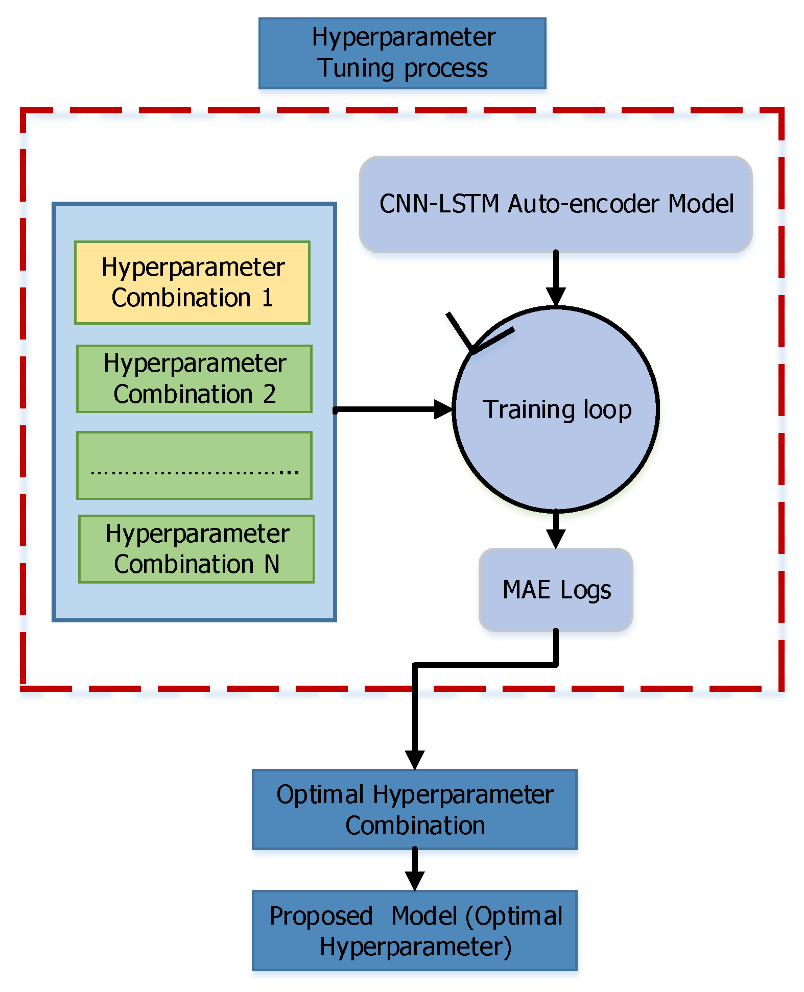
3.2. Hyperparameter Tuning
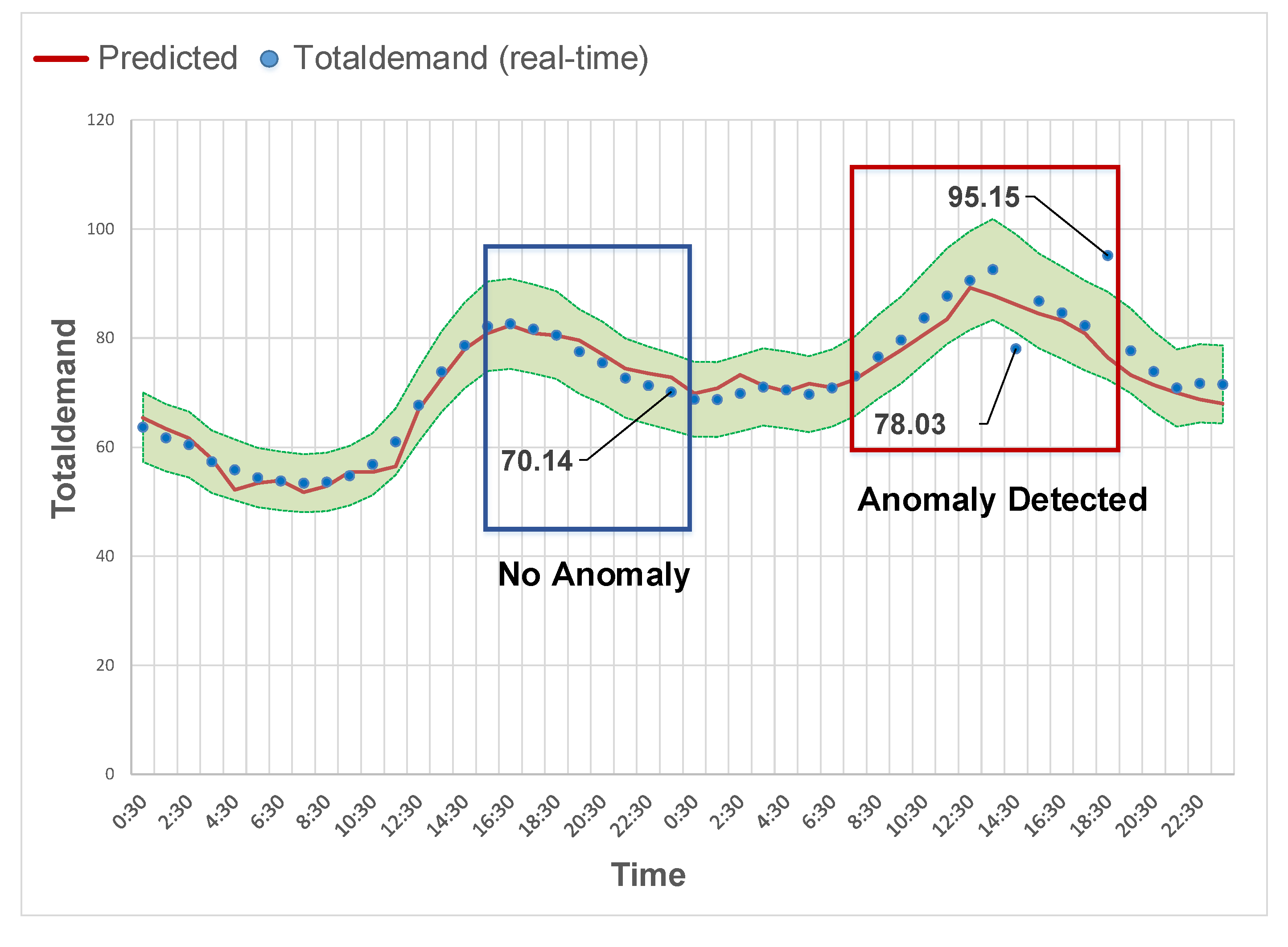
3.3. Real-Time Anomaly Detection Based on Accurate Forecasting
4. Results and Evaluation
4.1. Experimental Dataset
4.2. Error Matrix
4.3. Results
Attack Types
4.4. False Positive Rate
4.5. False Negative Rate
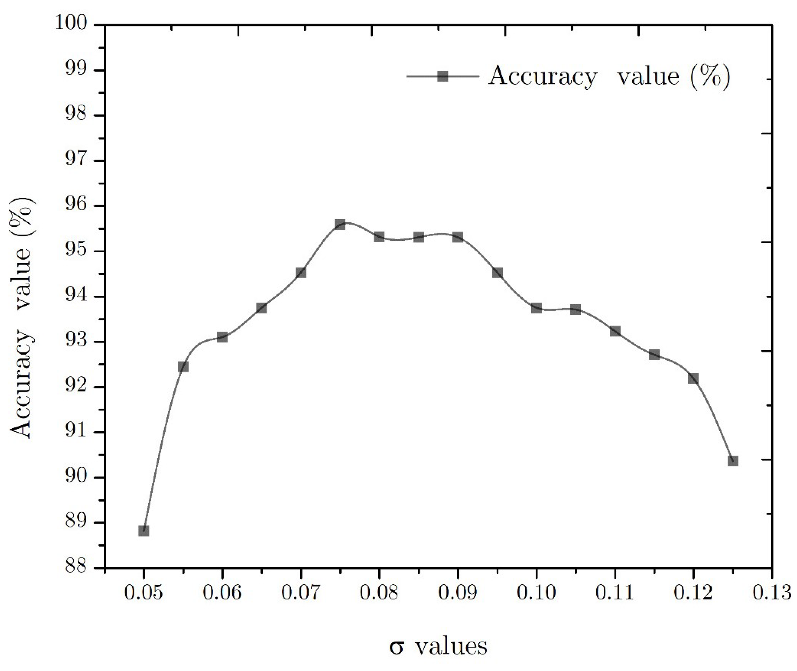
4.6. Accuracy Value
4.7. Discussion
5. Conclusions
Author Contributions
Funding
Institutional Review Board Statement
Informed Consent Statement
Data Availability Statement
Conflicts of Interest
Abbreviations
| SCADA | Supervisory Control and Data Acquisition |
| FDI | False Data Injection |
| PMU | Phasor Measurement Units |
| CNN | Convolutional Neural Network |
| LSTM | Long Short-term Memory |
| SVM | Support Vector Machine |
| ANN | Artificial Neural Networks |
| ARIMA | Autoregressive Integrated Moving Average |
| MLAD | Machine Learning based Anomaly Detection |
| FP | False Positive |
| FN | False Negative |
| ACC | Accuracy |
| AEMO | Australian Energy Market Operator |
| MAE | Mean Absolute Error |
| MAPE | Mean Absolute Percentage Error |
| MSE | Mean Squared Error |
| RMSE | Root Mean Squared Error |
References
- Güngör, V.C.; Sahin, D.; Kocak, T.; Ergüt, S.; Buccella, C.; Cecati, C.; Hancke, G.P. Smart grid technologies: Communication technologies and standards. IEEE Trans. Ind. Inform. 2011, 7, 529–539. [Google Scholar] [CrossRef] [Green Version]
- Wang, Y.; Pordanjani, I.R.; Xu, W. An event-driven demand response scheme for power system security enhancement. IEEE Trans. Smart Grid 2011, 2, 11–17. [Google Scholar] [CrossRef]
- Anwar, A.; Mahmood, A.N.; Pickering, M. Modeling and performance evaluation of stealthy false data injection attacks on smart grid in the presence of corrupted measurements. J. Comput. Syst. Sci. 2017, 83, 58–72. [Google Scholar] [CrossRef] [Green Version]
- Liang, G.; Weller, S.R.; Zhao, J.; Luo, F.; Dong, Z.Y. The 2015 Ukraine Blackout: Implications for False Data Injection Attacks. IEEE Trans. Power Syst. 2017, 32, 3317–3318. [Google Scholar] [CrossRef]
- Mallick, P. Cyber Attack on Kudankulam Nuclear Power Plant—A Wake Up Call; Vivekananda International Foundation: New Delhi, India, 2019. [Google Scholar]
- Lab, K. Threat Landscape for Industrial Automation Systems in H2 2019. ICS Cert 2019, 1–37. [Google Scholar]
- Morris, T.; Pan, S.; Lewis, J.; Moorhead, J.; Younan, N.; King, R.; Freund, M.; Madani, V. Cybersecurity risk testing of substation phasor measurement units and phasor data concentrators. In Proceedings of the Seventh Annual Workshop on Cyber Security and Information Intelligence Research, Oak Ridg, TN, USA, 12–14 October 2011. [Google Scholar] [CrossRef]
- Dondossola, G.; Szanto, J.; Masera, M.; Fovino, I.N. Effects of intentional threats to power substation control systems. Int. J. Crit. Infrastructures 2008, 4, 129–143. [Google Scholar] [CrossRef]
- Wang, J.W.; Rong, L.L. Cascade-based attack vulnerability on the US power grid. Saf. Sci. 2009, 47, 1332–1336. [Google Scholar] [CrossRef]
- Huang, Z.; Wang, C.; Zhu, T.; Nayak, A. Cascading failures in smart grid: Joint effect of load propagation and interdependence. IEEE Access 2015, 3, 2520–2530. [Google Scholar] [CrossRef]
- LaWell, M. The state of industrial: Robots. Ind. Week 2017, 266, 10–13. [Google Scholar]
- Stouffer, K.; Falco, J.; Scarfone, K. GUIDE to industrial control systems (ICS) security. Stuxnet Comput. Worm Ind. Control Syst. Secur. 2011, 800, 11–158. [Google Scholar]
- Anwar, A.; Mahmood, A.N. Vulnerabilities of Smart Grid State Estimation Against False Data Injection Attack. In Green Energy and Technology; Springer: Berlin/Heidelberg, Germany, 2014; pp. 411–428. [Google Scholar] [CrossRef] [Green Version]
- Inl/ext-06; Kuipers, D.; Fabro, M. Control Systems Cyber Security: Defense in Depth Strategies; Idaho National Laboratory: Idaho Falls, ID, USA, 2006; p. 8.
- Ameli, A.; Hooshyar, A.; El-saadany, E.F.; Youssef, A.M.; Member, S. Generation Control Systems. Attack Detection and Identification for Automatic Generation Control Systems. IEEE Trans. Power Syst. 2018, 33, 4760–4774. [Google Scholar] [CrossRef]
- Musleh, A.S.; Chen, G.; Dong, Z.Y. A Survey on the Detection Algorithms for False Data Injection Attacks in Smart Grids. IEEE Trans. Smart Grid 2020, 11, 2218–2234. [Google Scholar] [CrossRef]
- Huang, Y.F.; Werner, S.; Huang, J.; Kashyap, N.; Gupta, V. State estimation in electric power grids: Meeting new challenges presented by the requirements of the future grid. IEEE Signal Process. Mag. 2012, 29, 33–43. [Google Scholar] [CrossRef] [Green Version]
- College, D.S.; Helms, M.M.; Chapman, S. supply chain management Supply chain forecasting. Bus. Process Manag. J. 2000, 6, 392–407. [Google Scholar]
- Kim, K.J. Financial time series forecasting using support vector machines. Neurocomputing 2003, 55, 307–319. [Google Scholar] [CrossRef]
- Zhang, G.P.; Qi, M. Neural network forecasting for seasonal and trend time series. Eur. J. Oper. Res. 2005, 160, 501–514. [Google Scholar] [CrossRef]
- Gan, M.; Cheng, Y.; Liu, K.; Zhang, G.L. Seasonal and trend time series forecasting based on a quasi-linear autoregressive model. Appl. Soft Comput. J. 2014, 24, 13–18. [Google Scholar] [CrossRef]
- Pai, P.F.; Lin, K.P.; Lin, C.S.; Chang, P.T. Time series forecasting by a seasonal support vector regression model. Expert Syst. Appl. 2010, 37, 4261–4265. [Google Scholar] [CrossRef]
- Khashei, M.; Bijari, M.; Hejazi, S.R. Combining seasonal ARIMA models with computational intelligence techniques for time series forecasting. Soft Comput. 2012, 16, 1091–1105. [Google Scholar] [CrossRef]
- Chiemeke, S.C.; Oladipupo, A.O. African Journal of Science and Technology (AJST). Engineering 1982, 2, 101–107. [Google Scholar]
- Abhishek, K.; Singh, M.; Ghosh, S.; Anand, A. Weather Forecasting Model using Artificial Neural Network. Procedia Technol. 2012, 4, 311–318. [Google Scholar] [CrossRef] [Green Version]
- Abedinia, O.; Amjady, N.; Ghadimi, N. Solar energy forecasting based on hybrid neural network and improved metaheuristic algorithm. Comput. Intell. 2018, 34, 241–260. [Google Scholar] [CrossRef]
- Han, L.; Romero, C.E.; Yao, Z. Wind power forecasting based on principle component phase space reconstruction. Renew. Energy 2015, 81, 737–744. [Google Scholar] [CrossRef]
- Ahmed, A.; Khalid, M. An intelligent framework for short-term multi-step wind speed forecasting based on Functional Networks. Appl. Energy 2018, 225, 902–911. [Google Scholar] [CrossRef]
- Wang, H.; Lei, Z.; Zhang, X.; Zhou, B.; Peng, J. A review of deep learning for renewable energy forecasting. Energy Convers. Manag. 2019, 198, 111799. [Google Scholar] [CrossRef]
- Wang, H.Z.; Li, G.Q.; Wang, G.B.; Peng, J.C.; Jiang, H.; Liu, Y.T. Deep learning based ensemble approach for probabilistic wind power forecasting. Appl. Energy 2017, 188, 56–70. [Google Scholar] [CrossRef]
- Cheng, D.; Yang, F.; Xiang, S.; Liu, J. Financial time series forecasting with multi-modality graph neural network. Pattern Recognit. 2022, 121, 108218. [Google Scholar] [CrossRef]
- Ayoobi, N.; Sharifrazi, D.; Alizadehsani, R.; Shoeibi, A.; Gorriz, J.M.; Moosaei, H.; Khosravi, A.; Nahavandi, S.; Gholamzadeh Chofreh, A.; Goni, F.A.; et al. Time series forecasting of new cases and new deaths rate for COVID-19 using deep learning methods. Results Phys. 2021, 27, 104495. [Google Scholar] [CrossRef]
- Casado-Vara, R.; Martin del Rey, A.; Pérez-Palau, D.; De-la Fuente-Valentín, L.; Corchado, J.M. Web Traffic Time Series Forecasting Using LSTM Neural Networks with Distributed Asynchronous Training. Mathematics 2021, 9, 421. [Google Scholar] [CrossRef]
- Reda, H.T.; Anwar, A.; Mahmood, A. Comprehensive survey and taxonomies of false data injection attacks in smart grids: Attack models, targets, and impacts. Renew. Sustain. Energy Rev. 2022, 163, 112423. [Google Scholar] [CrossRef]
- Alfeld, S.; Zhu, X.; Barford, P. Data poisoning attacks against autoregressive models. In Proceedings of the 30th AAAI Conference on Artificial Intelligence, AAAI 2016, Phoenix, AZ, USA, 12–17 February 2016; pp. 1452–1458. [Google Scholar]
- Cui, M.; Wang, J.; Yue, M. Machine Learning-Based Anomaly Detection for Load Forecasting Under Cyberattacks. IEEE Trans. Smart Grid 2019, 10, 5724–5734. [Google Scholar] [CrossRef]
- Drayer, E.; Routtenberg, T. Detection of false data injection attacks in smart grids based on graph signal processing. IEEE Syst. J. 2019, 14, 1886–1896. [Google Scholar] [CrossRef] [Green Version]
- Zhao, J.; Zhang, G.; Dong, Z.Y.; Wong, K.P. Forecasting-aided imperfect false data injection attacks against power system nonlinear state estimation. IEEE Trans. Smart Grid 2016, 7, 6–8. [Google Scholar] [CrossRef]
- Sobhani, M.; Hong, T.; Martin, C. Temperature anomaly detection for electric load forecasting. Int. J. Forecast. 2020, 36, 324–333. [Google Scholar] [CrossRef]
- Nguyen, H.D.; Tran, K.P.; Thomassey, S.; Hamad, M. Forecasting and Anomaly Detection approaches using LSTM and LSTM Autoencoder techniques with the applications in supply chain management. Int. J. Inf. Manag. 2020, 57, 102282. [Google Scholar] [CrossRef]
- Fährmann, D.; Damer, N.; Kirchbuchner, F.; Kuijper, A. Lightweight Long Short-Term Memory Variational Auto-Encoder for Multivariate Time Series Anomaly Detection in Industrial Control Systems. Sensors 2022, 22, 2886. [Google Scholar] [CrossRef]
- Pasini, K.; Khouadjia, M.; Samé, A.; Trépanier, M.; Oukhellou, L. Contextual anomaly detection on time series: A case study of metro ridership analysis. Neural Comput. Appl. 2022, 34, 1483–1507. [Google Scholar] [CrossRef]
- Sun, M.; He, L.; Zhang, J. Deep learning-based probabilistic anomaly detection for solar forecasting under cyberattacks. Int. J. Electr. Power Energy Syst. 2022, 137, 107752. [Google Scholar] [CrossRef]
- Reda, H.T.; Anwar, A.; Mahmood, A.; Chilamkurti, N. Data-driven Approach for State Prediction and Detection of False Data Injection Attacks in Smart Grid. J. Mod. Power Syst. Clean Energy 2022, 1–13. [Google Scholar] [CrossRef]
- El Hariri, M.; Harmon, E.; Youssef, T.; Saleh, M.; Habib, H.; Mohammed, O. The IEC 61850 Sampled Measured Values Protocol: Analysis, Threat Identification, and Feasibility of Using NN Forecasters to Detect Spoofed Packets. Energies 2019, 12, 3731. [Google Scholar] [CrossRef] [Green Version]
- Australian Energy Market Operator. Available online: https://aemo.com.au (accessed on 15 February 2022).
- Sridhar, S.; Govindarasu, M. Model-based attack detection and mitigation for automatic generation control. IEEE Trans. Smart Grid 2014, 5, 580–591. [Google Scholar] [CrossRef]


| Hyperparameter Type | Hyperparameter Value |
|---|---|
| Conv1d Filter number | 32 |
| Conv1d Kernel size | 3 |
| Maxpooling1d pool size | 2 |
| LSTM unit number | 220 |
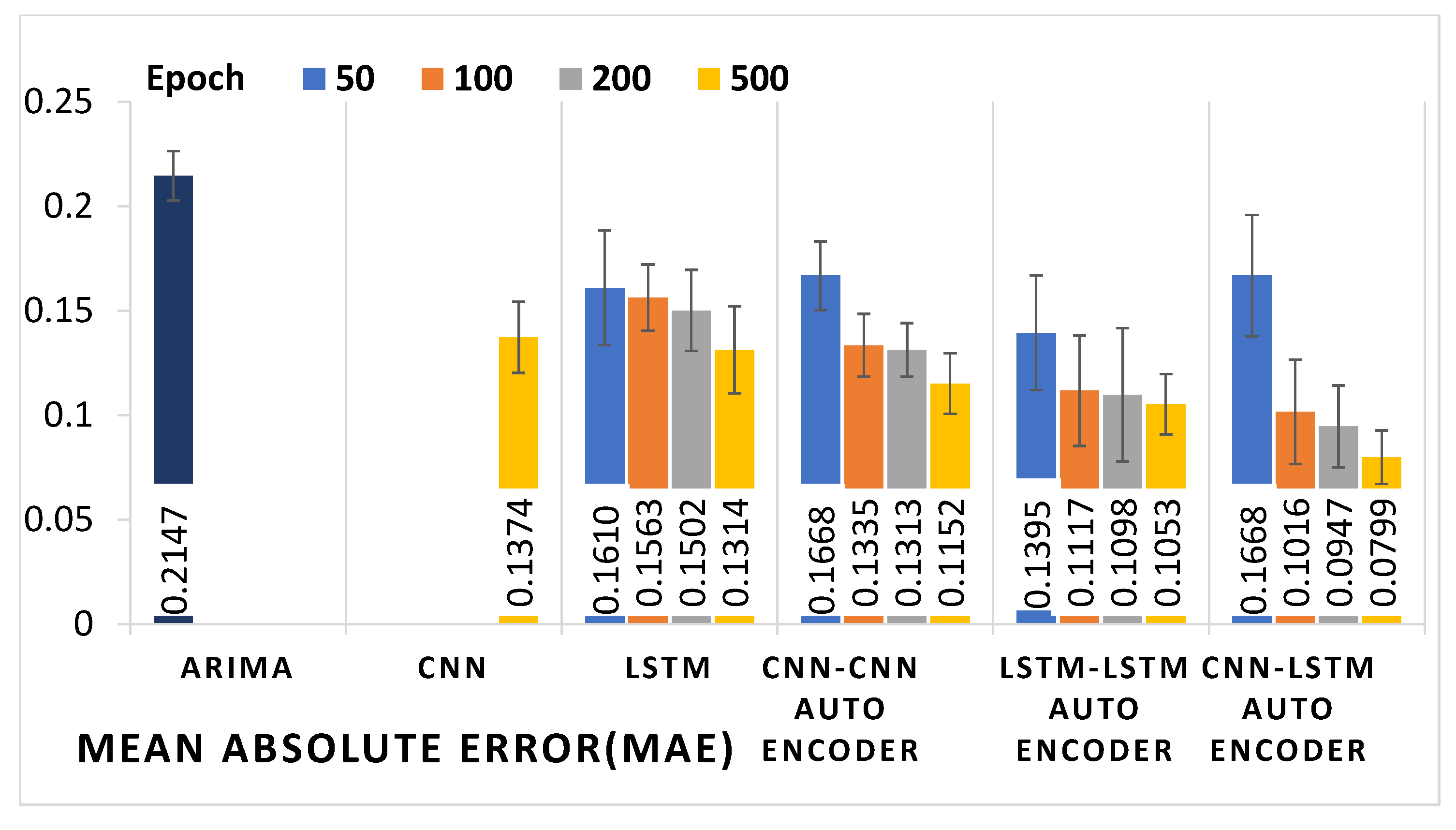
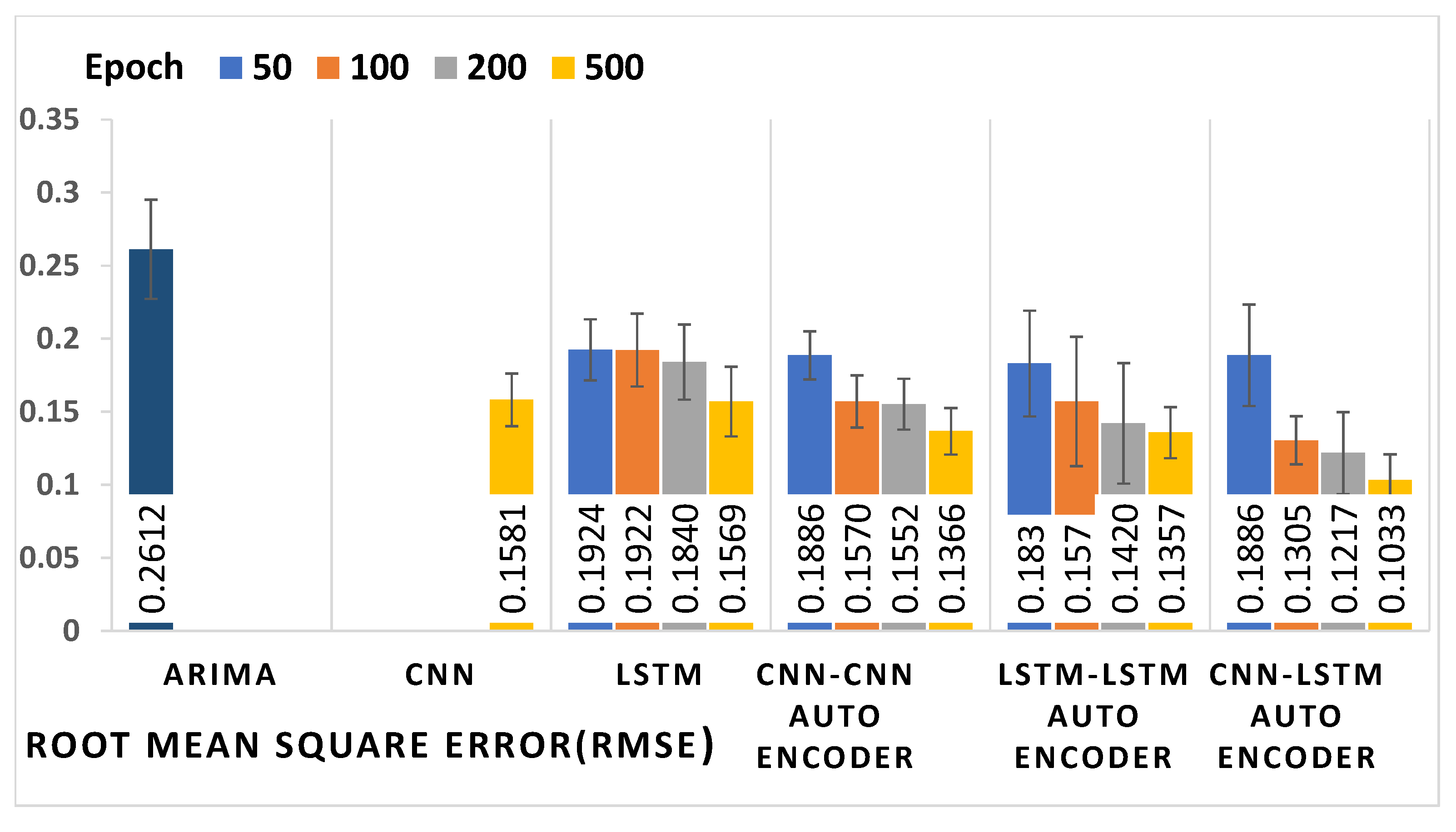
| Models | Epoch | MAE | MAPE (%) | MSE | RMSE |
|---|---|---|---|---|---|
| ARIMA | - | 0.2147 0.0118 | 32.68 2.69 | 0.0682 0.0014 | 0.2612 0.0339 |
| CNN | 500 | 0.1374 0.0171 | 22.98 0.86 | 0.0249 0.0003 | 0.1581 0.0181 |
| LSTM | 50 | 0.1610 0.0274 | 27.24 1.32 | 0.0370 0.0004 | 0.1924 0.0209 |
| 100 | 0.1563 0.0159 | 24.39 0.85 | 0.0369 0.0006 | 0.1922 0.0249 | |
| 200 | 0.1502 0.0194 | 23.09 0.92 | 0.0338 0.0006 | 0.1840 0.0257 | |
| 500 | 0.1314 0.0208 | 21.52 0.97 | 0.2461 0.0005 | 0.1569 0.0238 | |
| CNN-CNN | 50 | 0.1668 0.0165 | 26.15 0.87 | 0.0355 0.0002 | 0.1886 0.0165 |
| Auto-encoder | 100 | 0.1335 0.0150 | 22.18 0.72 | 0.0246 0.0003 | 0.1570 0.0179 |
| 200 | 0.1313 0.0128 | 21.69 0.65 | 0.0240 0.0003 | 0.1552 0.0174 | |
| 500 | 0.1152 0.0145 | 18.08 0.69 | 0.0186 0.0002 | 0.1366 0.0159 | |
| LSTM-LSTM | 50 | 0.1395 0.0275 | 22.49 2.86 | 0.0334 0.0013 | 0.1830 0.0362 |
| Auto-encoder | 100 | 0.1117 0.0264 | 17.65 1.16 | 0.0246 0.0019 | 0.1570 0.0443 |
| 200 | 0.1098 0.0319 | 13.07 1.82 | 0.0201 0.0016 | 0.1420 0.0412 | |
| 500 | 0.1053 0.0144 | 12.09 0.74 | 0.0184 0.0003 | 0.1357 0.0175 | |
| CNN-LSTM | 50 | 0.1668 0.0291 | 25.91 2.95 | 0.0357 0.0012 | 0.1886 0.0347 |
| Auto-encoder | 100 | 0.1016 0.0250 | 15.96 1.45 | 0.0170 0.0002 | 0.1305 0.0165 |
| 200 | 0.0947 0.0196 | 10.87 1.22 | 0.0148 0.0007 | 0.1217 0.0281 | |
| 500 | 0.0799 0.0128 | 8.07 0.62 | 0.0106 0.0003 | 0.1033 0.0176 |
Publisher’s Note: MDPI stays neutral with regard to jurisdictional claims in published maps and institutional affiliations. |
© 2022 by the authors. Licensee MDPI, Basel, Switzerland. This article is an open access article distributed under the terms and conditions of the Creative Commons Attribution (CC BY) license (https://creativecommons.org/licenses/by/4.0/).
Share and Cite
Mahi-al-rashid, A.; Hossain, F.; Anwar, A.; Azam, S. False Data Injection Attack Detection in Smart Grid Using Energy Consumption Forecasting. Energies 2022, 15, 4877. https://doi.org/10.3390/en15134877
Mahi-al-rashid A, Hossain F, Anwar A, Azam S. False Data Injection Attack Detection in Smart Grid Using Energy Consumption Forecasting. Energies. 2022; 15(13):4877. https://doi.org/10.3390/en15134877
Chicago/Turabian StyleMahi-al-rashid, Abrar, Fahmid Hossain, Adnan Anwar, and Sami Azam. 2022. "False Data Injection Attack Detection in Smart Grid Using Energy Consumption Forecasting" Energies 15, no. 13: 4877. https://doi.org/10.3390/en15134877
APA StyleMahi-al-rashid, A., Hossain, F., Anwar, A., & Azam, S. (2022). False Data Injection Attack Detection in Smart Grid Using Energy Consumption Forecasting. Energies, 15(13), 4877. https://doi.org/10.3390/en15134877