
A Comprehensive Energy Model for an Optimal Design of a Hybrid Refrigerated Van

 ,
,  ,
,  , , and
Abstract
:1. Introduction
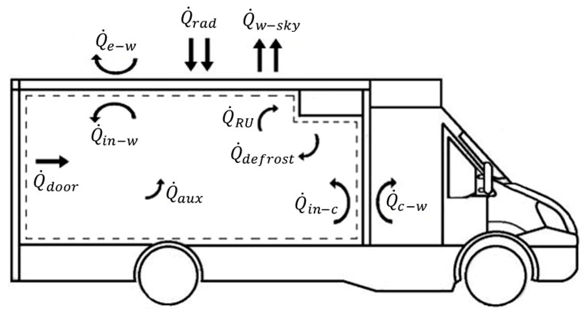
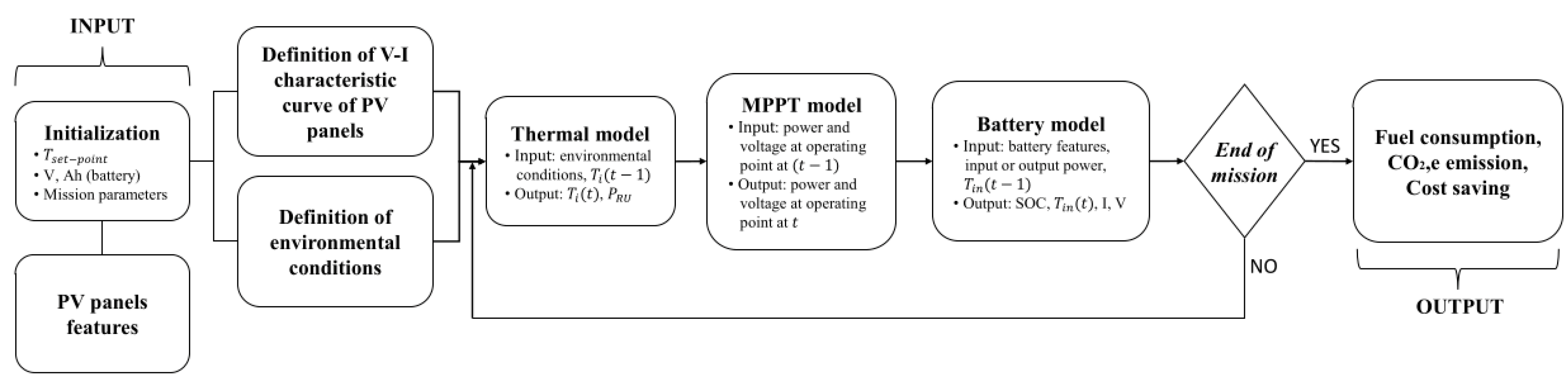
2. Comprehensive Energy Model
3. Results and Discussion
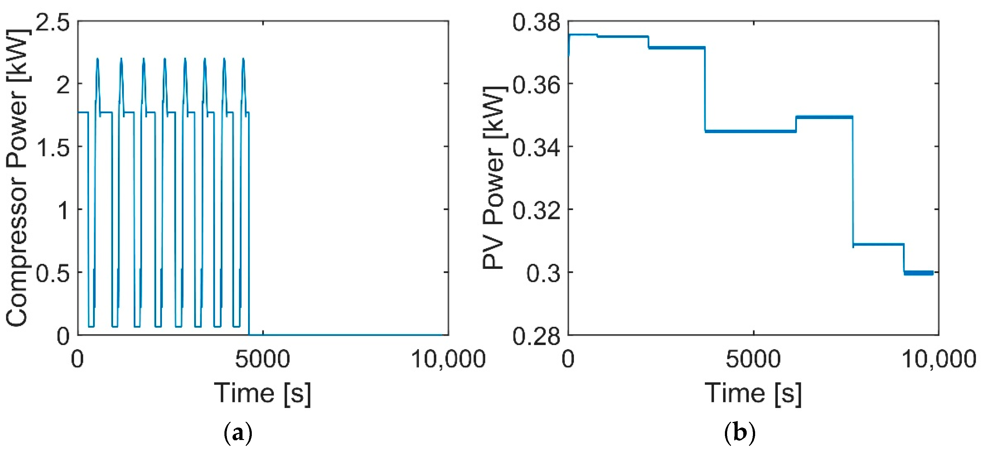
3.1. Single-Delivery Scenario
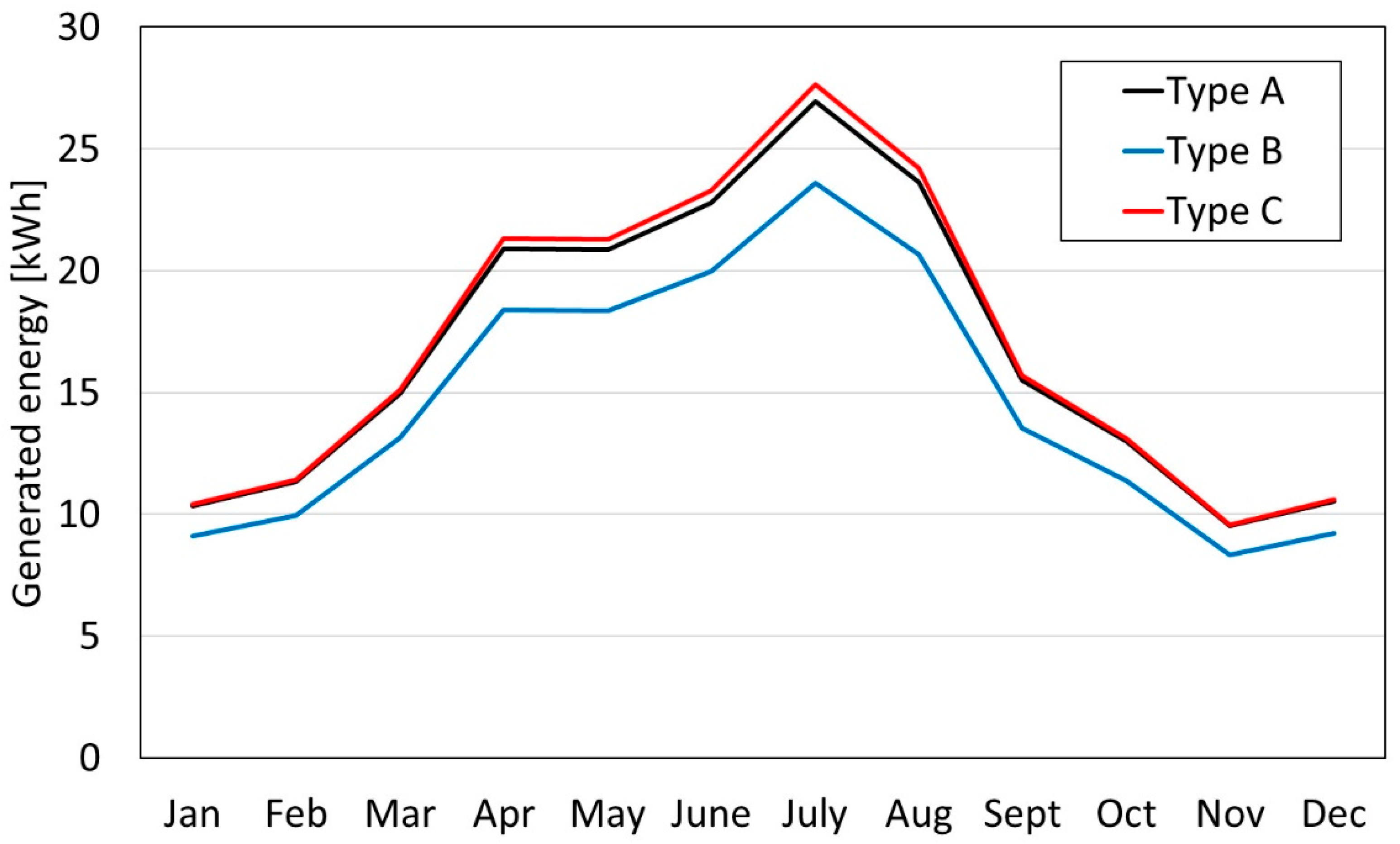
3.1.1. Selection of PV Panels
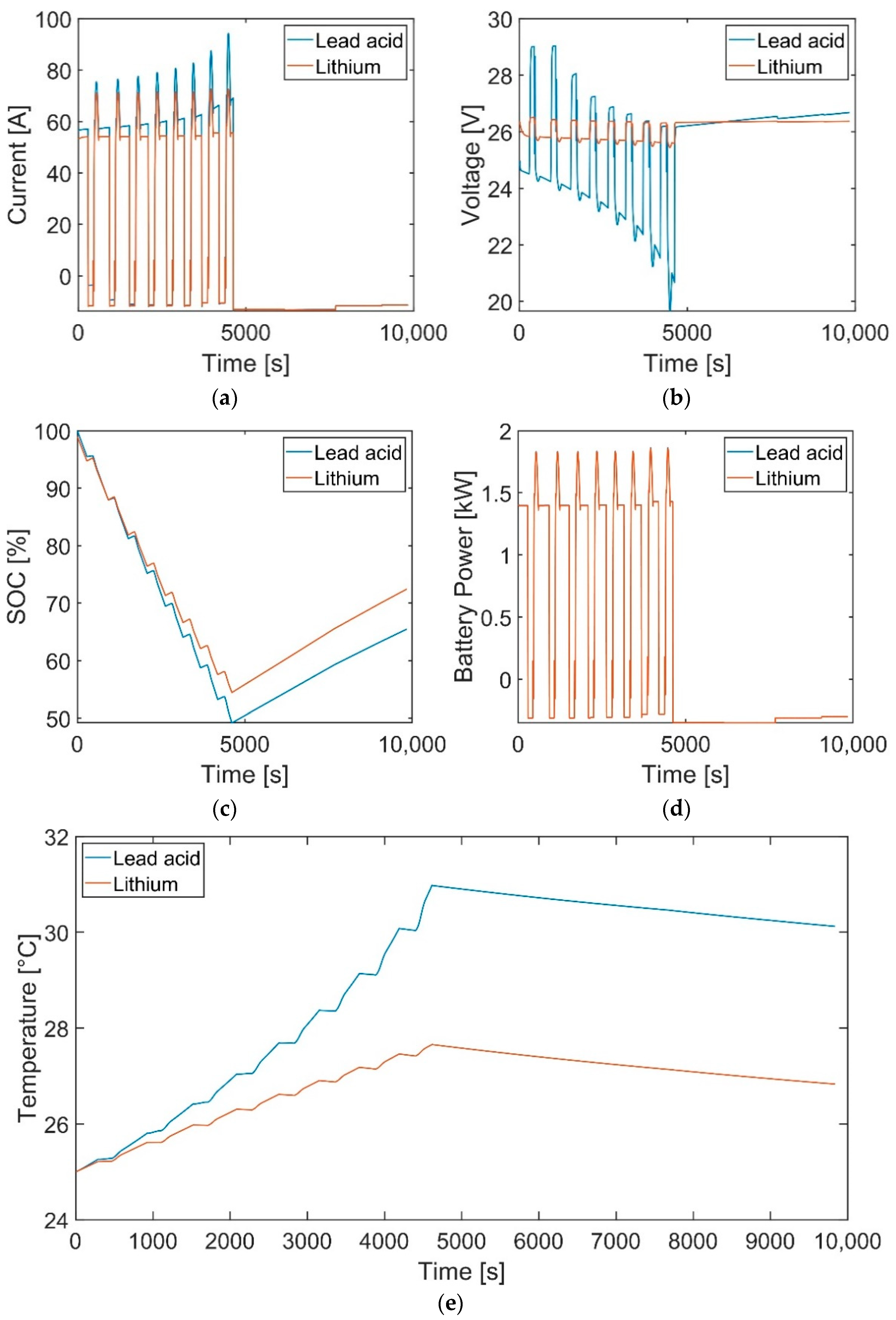
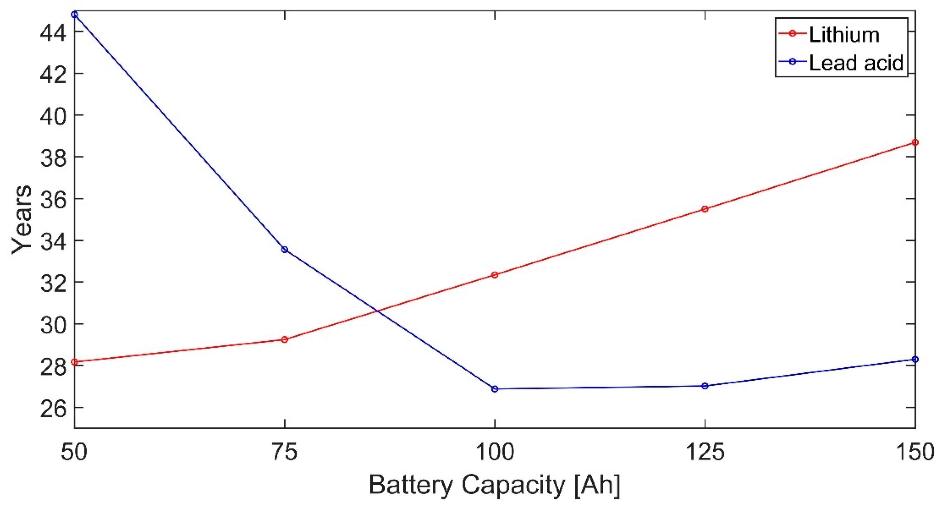
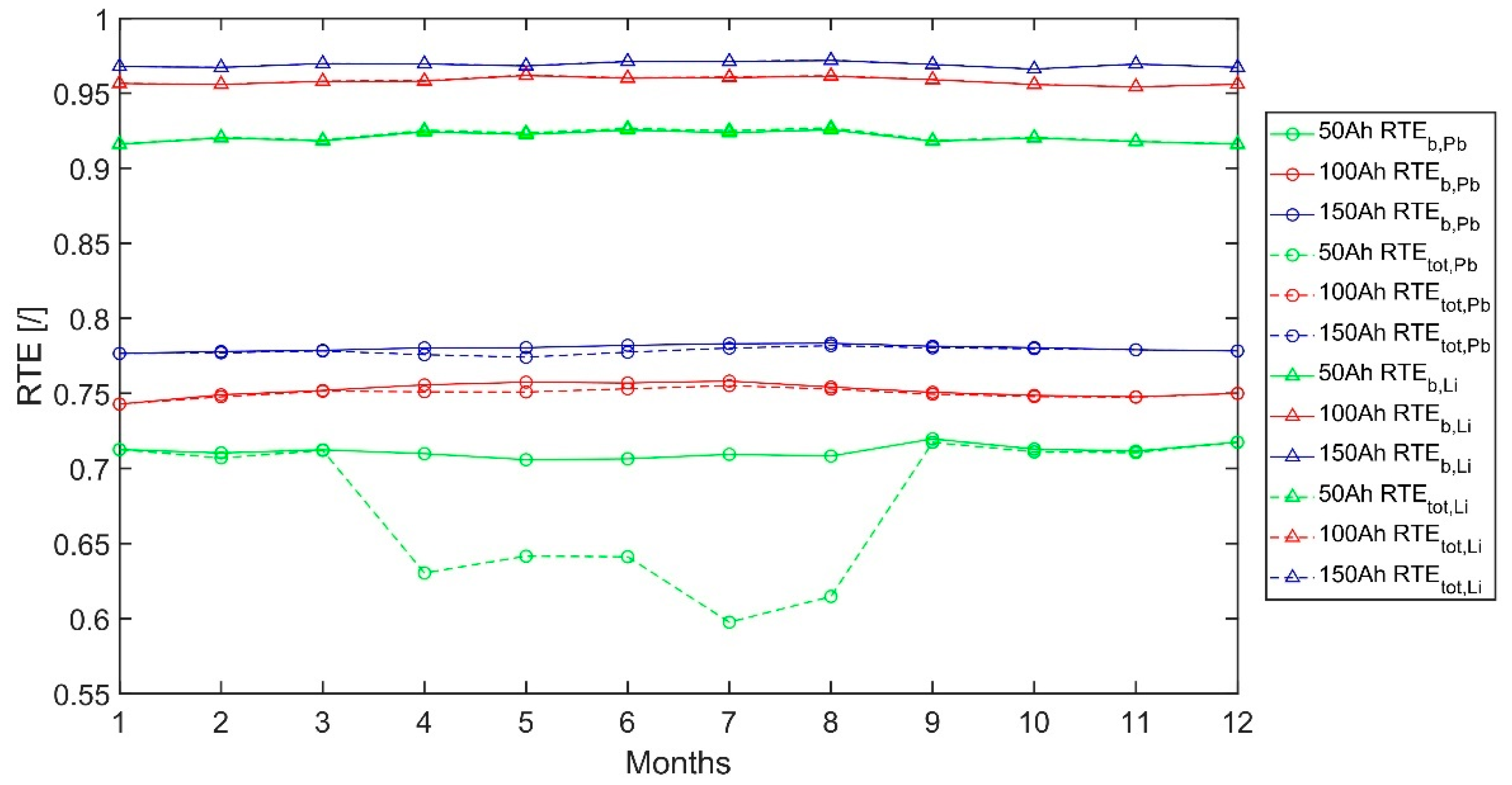
3.1.2. Selection of Batteries
3.1.3. Overall Results
3.2. Multiple-Deliveries Scenario
4. Conclusions
Author Contributions
Funding
Institutional Review Board Statement
Informed Consent Statement
Conflicts of Interest
Nomenclature
| Symbols | |
| A | amplitude of the exponential area [V] |
| B | constant of time in the exponential area [Ah−1] |
| c | specific heat [J kg−1 K−1] |
| Cd | coefficient of aerodynamic drag [-] |
| Cinf | infiltration coefficient [m1/2 s−1] |
| C | cost [€] |
| CorrR | resistance correction parameter [Ah−1] |
| CorrK | polarization constant correction parameter [A−1] |
| Cr | rolling resistance coefficient [-] |
| Cu | unit cost of methane [€ kg−1] |
| d | distance [m] |
| Den | engine displacement [m−3] |
| E | electric energy [kWh] |
| Exp | exponential voltage [V] |
| emission factor [kgCO2,e MJ−1] | |
| F | fuel consumption [kg] |
| FR | instantaneous rate of fuel consumption [kg s−1] |
| g | gravity [m s−2] |
| G | solar radiation [W m−2] |
| h | convective heat transfer coefficient- [W m−2 K−1] |
| H | door’s height [m] |
| i | current [A] |
| * | filtered current [A] |
| it | actual charge of the battery [Ah] |
| j | specific enthalpy [kJ kg−1] |
| k | engine friction value [-] |
| K | polarization constant [V Ah−1] |
| l | transport load [kg] |
| LHV | lower heating value [kJ kg−1 or MJ kh−1] |
| m | mass [kg] |
| mass flow rate [kg s−1] | |
| Nen | engine rotation speed [rps] |
| P | electric power [W] |
| Q | battery capacity [Ah] |
| heat transfer [W] | |
| heat flow rate [W m−2] | |
| R | internal resistance of the battery [Ω] |
| RTE | Round Trip Efficiency [-] |
| s | width [m] |
| S | surface [m2] |
| SOC | State Of Charge [%] |
| T | temperature [°C or K] |
| t | time [s] |
| v | speed [m s−1] |
| V | voltage [V] |
| constant voltage [V] | |
| Greek symbols | |
| η | efficiency [-] |
| ηi | Coulombic efficiency [-] |
| σ | Stephan–Boltzmann constant [W m−2 K−4] |
| ρ | density [kg m−3] |
| τ | characteristic time constant of the considered battery [s] |
| Subscripts | |
| AG | air gap |
| amb | ambient |
| aux | auxiliary components |
| b | battery |
| B | body |
| back | back side |
| c | cabinet |
| conv | conversion |
| defrost | defrost system |
| door | door |
| drive | drive |
| e | external |
| en | engine |
| front | front side |
| fuel | fuel |
| g | global |
| in | inside |
| Li | Lithium battery |
| mec | mechanical |
| mp | maximum power |
| nom | nominal |
| oc | open circuit |
| Pb | lead-acid battery |
| PV | photovoltaic |
| rad | radiation |
| real | real or indicated |
| ref | reference |
| Reintegrated | reintegrated from the grid |
| roof | roof |
| RU | refrigeration unit |
| sc | short circuit |
| sol | solar |
| sky | sky |
| w | wall |
| Abbreviations | |
| CO2,e | Carbon dioxide equivalent |
| MPPT | Maximum Power Point Tracking |
| PV | Photovoltaic |
Appendix A. Refrigerated Van and PV System Features

| Parameter | Characteristics |
|---|---|
| Engine (F1CFA401A) | Four-stroke bi-fuel spark ignition (petrol-methane) maximum power (methane): 100 kW (136 CV) @ 2730–3500 rpm maximum torque (methane): 350 N·m @ 1500–2730 rpm Displacement: 2998 cm3 |
| Refrigerated cabin | Reinforced isothermal class F (thermal transmittance of the walls between 0.29 and 0.4 W m−2K−1), minimum temperature inside the cabin of −20 °C |
| Refrigeration unit | R-452A refrigerant, hermetic compressor with inverter (30 to 80 Hz) |
| Refrigeration unit power supply | Electric mains or dedicated auxiliary alternator, directly driven by the heat engine |
| Parameter | Body | Polyurethane | Glass Fiber Reinforced Polymer (GRFP) |
|---|---|---|---|
| Heat transfer transmittance, λ (W m−1 K−1) | 60 | 0.024 | 0.64 |
| Width, s (m) | 0.005 | 0.064 | 0.002 |
| Density, ρ (kg m−3) | 2700 | 40 | 1800 |
| Specific heat capacity, c (J kg−1 K−1) | 900 | 1400 | 1255 |
| Parameter | Type A | Type B | Type C |
|---|---|---|---|
| Technology | HJT | Monocrystalline | Monocrystalline |
| Peak power [W] | 120 | 108 | 52 |
| Voc [V] | 17.3 | 15.3 | 10.9 |
| Vmp [V] | 14 | 12.6 | 9.1 |
| imp [A] | 8.6 | 8.6 | 5.7 |
| isc [A] | 9 | 9 | 6 |
| Dimensions [mm] | 1046 × 683 | 1046 × 683 | 1109 × 293 |
| Weight [kg] | 1.7 | 1.7 | 0.8 |
| Parameter | Value |
|---|---|
| Nominal power [VA/W] | 3000/3000 |
| Voltage [VAC] | 230 |
| AC Voltage regulation (battery mode) [VAC] | 230 ± 5% 170–280 (For Personal Computers) 280 (For Home Appliances) |
| Peak power [VA] | 6000 |
| Efficiency peak [/] | 90% to 93% |
| Transfer time [ms] | 10 (For Personal Computers) 20 (For Home Appliances) |
| Waveshape | PURE WAVE |
| Battery/charge voltage [VDC] | 24/27 |
| Overcharge protection [VDC] | 33 |
| Type of charge controller | MPPT |
| Maximum capacity PV [W] | 1500 |
| Maximum PV array open-circuit voltage [VDC] | 145 |
| PV Array MPPT Voltage Range [VDC] | 30 to 115 |
| Maximum charge current: solar and AC/rest [A] | 60/120 |
| Relative humidity | 5% to 95% |
| Operating/storage temperature [°C] | −10 to 50/−15 to 60 |
Appendix B
| Type of Heat Transfer | Equation |
|---|---|
| Convective between the walls’ external surface and the external air [34] | |
| Convective between the walls’ external surface and the air inside the driver’s cabin [34] | |
| Incident solar radiation [34] | |
| Radiative with the celestial vault (the vehicle is considered a small convex object placed inside a cavity) [34] | |
| Convective between the internal air and the surface of the inner wall bordering the outside | |
| Convective between the internal air and the walls’ inner surface bordering the driver’s cabin | |
| Internal due to the auxiliaries | |
| Door opening (≠0 only in the goods loading/unloading phases, known duration) [35] | where, |
| Defrost system, given by electrical resistances (≠0 only during activation, known duration) | |
| Cooling capacity of the refrigeration system |
| Condition | Equation |
|---|---|
| With the ambient | |
| With the cabin | |
| With the internal air (wall that exchanges with the ambient) | |
| With the internal air (wall that exchanges with the driver’s cabin) | |
| Between two adjacent layers of the stratigraphy (i and j) |
| Density | Width | Specific Heat Capacity | Absorptivity (Front Side) | Absorptivity (Back Side) | Emissivity |
|---|---|---|---|---|---|
| 2700 kg m−3 | 0.003 m | 900 J kg−1 K−1 | 0.72 | 0.2 | 0.91 |
Appendix C
Appendix C.1. Lithium Battery
- is the constant voltage of the battery [V];
- K is the Polarization constant [V A−1h−1] or Polarization resistance [Ω];
- Q is the battery capacity [Ah];
- it is the actual charge of the battery [Ah];
- A is the width of the exponential area [V];
- B is the constant of time in the exponential area [Ah−1];
- R is the internal resistance of the battery [Ω];
- i is the current [A];
- i* is the filtered current [A].
Appendix C.2. Lead-Acid Battery
- Q(i) is the battery capacity, in Ah, at the discharge current i;
- Qnom is the nominal battery capacity at a reference discharge current i0;
- Q(i2) and Q(i1) are two different battery capacities at different discharge rates i2 and i1;
- Exp (t) is the exponential voltage [V], given by:
Appendix C.3. Generalization of the Model
References
- AssoGasMetano. Available online: https://www.assogasmetano.it/prezzo-medio-nazionale-2018/ (accessed on 6 March 2020).
- Barth, M.; Younglove, T.; Scora, G. Development of a Heavy-Duty Diesel Modal Emissions and Fuel Consumption Model. 2005. UC Berkeley California Partners for Advanced Transportation Technology. Available online: https//escholarship.org/uc/item/67f0v3zf (accessed on 2 June 2022).
- Blasko, V.; Bendapudi, S.; Oggianu, S.M. Solar Power Assisted Transport Refrigeration Systems, Transport Refrigeration Units and Methods for Same. U.S. Patent US20130000342A1, 3 January 2013. [Google Scholar]
- Cenex. Refrigerated Transport Insights-A ZERO White Paper; Cenex: Loughborough, UK, 2021. [Google Scholar]
- Chang, W.-Y. The State of Charge Estimating Methods for Battery: A Review. ISRN Appl. Math. 2013, 2013, 953792. [Google Scholar] [CrossRef]
- Citarella, B.; Viscito, L.; Mochizuki, K.; Mauro, A.W. Multi-criteria (thermo-economic) optimization and environmental analysis of a food refrigeration system working with low environmental impact refrigerants. Energy Convers. Manag. 2022, 253, 115152. [Google Scholar] [CrossRef]
- Franceschetti, A.; Honhon, D.; Van Woensel, T.; Bektaş, T.; Laporte, G. The time-dependent pollution-routing problem. Transp. Res. Part B Methodol. 2013, 56, 265–293. [Google Scholar] [CrossRef] [Green Version]
- Górny, K.; Stachowiak, A.; Tyczewski, P.; Zwierzycki, W. Lubricity of selected oils in mixtures with the refrigerants R452A, R404A, and R600a. Tribol. Int. 2019, 134, 50–59. [Google Scholar] [CrossRef]
- Infante Ferreira, C.; Kim, D.-S. Techno-economic review of solar cooling technologies based on location-specific data. Int. J. Refrig. 2014, 39, 23–37. [Google Scholar] [CrossRef]
- ISPRA. 2019. Available online: https://www.isprambiente.gov.it/files2019/pubblicazioni/rapporti/R_303_19_gas_serra_settore_elettrico.pdf (accessed on 6 March 2020).
- Kim, D.S.; Infante Ferreira, C.A. Solar refrigeration options–a state-of-the-art review. Int. J. Refrig. 2008, 31, 3–15. [Google Scholar] [CrossRef]
- Ladha-Sabur, A.; Bakalis, S.; Fryer, P.J.; Lopez-Quiroga, E. Mapping energy consumption in food manufacturing. Trends Food Sci. Technol. 2019, 86, 270–280. [Google Scholar] [CrossRef]
- Lawton, R.; Curlin, J.S.; Clark, W. Technology Brief IIR-UN Environment Cold Chain Brief on Transport Refrigeration; International Institute of Refrigeration (IIFIIR): Paris, Prance, 2018; Available online: https://wedocs.unep.org/bitstream/handle/20.500.11822/32571/8142Transpor_Ref_EN.pdf?sequence=1&isAllowed=y (accessed on 2 June 2022).
- Lazzarin, R.M. Solar cooling: PV or thermal? A thermodynamic and economical analysis. Int. J. Refrig. 2014, 39, 38–47. [Google Scholar] [CrossRef]
- Lazzarin, R.M.; Noro, M. Past, present, future of solar cooling: Technical and economical considerations. Sol. Energy 2018, 172, 2–13. [Google Scholar] [CrossRef]
- Li, G. Comprehensive investigation of transport refrigeration life cycle climate performance. Sustain. Energy Technol. Assess. 2017, 21, 33–49. [Google Scholar] [CrossRef]
- Mahmoudi, M.; Dehghan, M.; Haghgou, H.; Keyanpour-Rad, M. Techno-economic performance of photovoltaic-powered air-conditioning heat pumps with variable-speed and fixed-speed compression systems. Sustain. Energy Technol. Assess. 2021, 45, 101113. [Google Scholar] [CrossRef]
- Maiorino, A.; Petruzziello, F.; Aprea, C. Refrigerated Transport: State of the Art, Technical Issues, Innovations and Challenges for Sustainability. Energies 2021, 14, 7237. [Google Scholar] [CrossRef]
- Meneghetti, A.; Ceschia, S. Energy-efficient frozen food transports: The Refrigerated Routing Problem. Int. J. Prod. Res. 2020, 58, 4164–4181. [Google Scholar] [CrossRef]
- Mota-Babiloni, A.; Makhnatch, P. Predictions of European refrigerants place on the market following F-gas regulation restrictions. Int. J. Refrig. 2021, 127, 101–110. [Google Scholar] [CrossRef]
- Nasuta, D.; Srichai, R.; Zhang, M.; Martin, C.; Muehlbauer, J. Life Cycle Climate Performance Model for Transport Refrigeration/Air Conditioning Systems. ASHRAE Trans. 2014, 120, 1P–8P. [Google Scholar]
- Njoroge, P.; Ndunya, L.S.; Kabiru, P. Hybrid Solar-Wind Power System for Truck Refrigeration. In Proceedings of the 2018 IEEE PES/IAS PowerAfrica, Cape Town, South Africa, 28–29 June 2018; pp. 1–9. [Google Scholar]
- De Novaes Pires Leite, G.; Weschenfelder, F.; Araújo, A.M.; Villa Ochoa, Á.A.; da Franca Prestrelo Neto, N.; Kraj, A. An economic analysis of the integration between air-conditioning and solar photovoltaic systems. Energy Convers. Manag. 2019, 185, 836–849. [Google Scholar] [CrossRef]
- Rai, A.; Tassou, S.A. Energy demand and environmental impacts of alternative food transport refrigeration systems. Energy Procedia 2017, 123, 113–120. [Google Scholar] [CrossRef]
- Reda, F.; Paiho, S.; Pasonen, R.; Helm, M.; Menhart, F.; Schex, R.; Laitinen, A. Comparison of solar assisted heat pump solutions for office building applications in Northern climate. Renew. Energy 2020, 147, 1392–1417. [Google Scholar] [CrossRef]
- Riva, C.; Roumpedakis, T.C.; Kallis, G.; Rocco, M.V.; Karellas, S. Life cycle analysis of a photovoltaic driven reversible heat pump. Energy Build. 2021, 240, 110894. [Google Scholar] [CrossRef]
- Salilih, E.M.; Birhane, Y.T. Modelling and performance analysis of directly coupled vapor compression solar refrigeration system. Sol. Energy 2019, 190, 228–238. [Google Scholar] [CrossRef]
- Sarbu, I.; Sebarchievici, C. Review of solar refrigeration and cooling systems. Energy Build. 2013, 67, 286–297. [Google Scholar] [CrossRef]
- Sovacool, B.K.; Bazilian, M.; Griffiths, S.; Kim, J.; Foley, A.; Rooney, D. Decarbonizing the food and beverages industry: A critical and systematic review of developments, sociotechnical systems and policy options. Renew. Sustain. Energy Rev. 2021, 143, 110856. [Google Scholar] [CrossRef]
- Stoecker, W.F. Industrial Refrigeration Handbook; McGraw-Hill Education: New York, NY, USA, 1998. [Google Scholar]
- Su, P.; Ji, J.; Cai, J.; Gao, Y.; Han, K. Dynamic simulation and experimental study of a variable speed photovoltaic DC refrigerator. Renew. Energy 2020, 152, 155–164. [Google Scholar] [CrossRef]
- Tassou, S.A.; De-Lille, G.; Ge, Y.T. Food transport refrigeration—Approaches to reduce energy consumption and environmental impacts of road transport. Appl. Therm. Eng. 2009, 29, 1467–1477. [Google Scholar] [CrossRef] [Green Version]
- Torregrosa-Jaime, B.; Bjurling, F.; Corberán, J.M.; Di Sciullo, F.; Payá, J. Transient thermal model of a vehicle’s cabin validated under variable ambient conditions. Appl. Therm. Eng. 2015, 75, 45–53. [Google Scholar] [CrossRef] [Green Version]
- Tremblay, O.; Dessaint, L.A. Experimental validation of a battery dynamic model for EV applications. World Electr. Veh. J. 2009, 3, 289–298. [Google Scholar] [CrossRef] [Green Version]
- UNECE. Climate Change and Sustainable Transport; UNECE: Geneva, Switzerland, 2021. [Google Scholar]
- Wu, X.; Hu, S.; Mo, S. Carbon footprint model for evaluating the global warming impact of food transport refrigeration systems. J. Clean. Prod. 2013, 54, 115–124. [Google Scholar] [CrossRef]
- Yang, Z.; Tate, J.E.; Morganti, E.; Shepherd, S.P. Real-world CO2 and NOX emissions from refrigerated vans. Sci. Total Environ. 2021, 763, 142974. [Google Scholar] [CrossRef]


| Parameter | Model | Test |
|---|---|---|
| Total distance (km) | 90.2 | |
| Total time (min) | 63 | |
| Departure | 11.10 | |
| Drive (kg) | 10.02 | Not applicable |
| Refrigeration (kg) | 0.46 | Not applicable |
| Total consumption (kg) | 10.5 | 10.1 |
| Total cost (€) | 9.96 | 10.0 |
| Total CO2 emissions (kg) | 28.1 | 28.2 |
| Code | Address | Coordinates |
|---|---|---|
| O | Via Santa Maria La Neve, Tramonti (SA) | 40.70, 14.66 |
| D1 | Via Benedetto Croce 63, Avellino (AV) | 40.92, 14.78 |
| D2 | Corso Giuseppe Garibaldi 12, Castellammare di Stabia (NA) | 40.70, 14.48 |
| D3 | Via Salvatore D’Alessandro 42, Nocera Inferiore (SA) | 40.75, 14.63 |
| Component | Unit Cost [€] | Units | Total Cost [€] |
|---|---|---|---|
| MC4 connectors | 4.80 | 1 | 4.80 |
| Extension cable | 1.20 | 14 | 16.80 |
| Double-sided adhesive | 18.00 | 5 | 90.00 |
| Inverter-MPPT | 473.72 | 1 | 473.72 |
| 24 V 100 Ah battery | 480.00 | 1 | 480.00 |
| Total | 1065.32 | ||
| PV Panel | Unit Cost [€] | Units | Cost PV Panels [€] | Total Cost [€] |
|---|---|---|---|---|
| Type A | 430.00 | 5 | 2150.00 € | 3215.32 |
| Type B | 290.00 | 5 | 1450.00 € | 2515.32 |
| Type C | 260.00 | 12 | 3120.00 € | 4185.32 |
| Parameter | Baseline | Type A | Type B | Type C |
|---|---|---|---|---|
| Investment cost [€] | NA | 3215.32 | 2515.32 | 4185.32 |
| Power grid cost [€] | NA | 19.97 | 20.82 | 19.79 |
| Annual costs [€] | 1606.46 | 1488.46 | 1492.68 | 1488.06 |
| Net Present Value [€] | NA | 118.00 | 113.78 | 118.40 |
| Payback period [years] | NA | 27 | 22 | 36 |
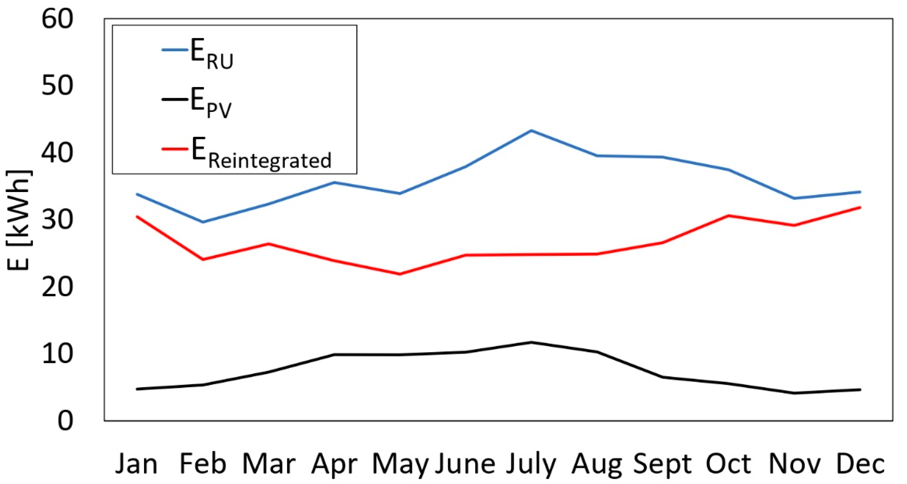
| Parameter | Jan | Feb | Mar | Apr | May | Jun | Jul | Aug | Sep | Oct | Nov | Dec |
|---|---|---|---|---|---|---|---|---|---|---|---|---|
| Distance [km] | 72.10 | |||||||||||
| Time [min] | 77.00 | |||||||||||
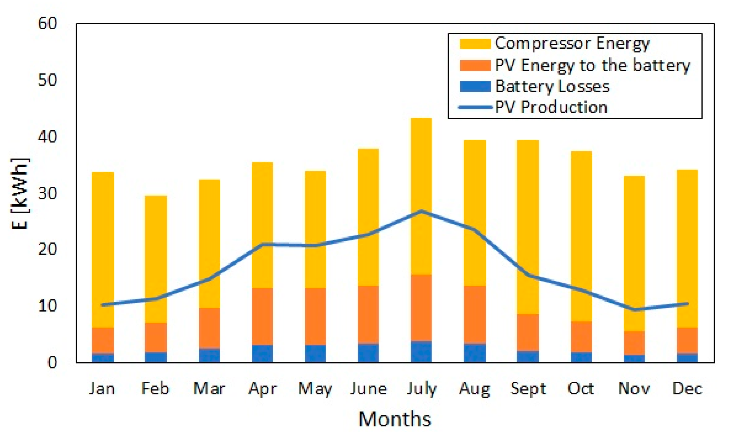
| ERU [kWh] | 33.7 | 29.1 | 32.4 | 35.5 | 34.0 | 38.0 | 43.3 | 39.6 | 39.1 | 37.7 | 33.0 | 33.8 |
| EPS [kWh] | 5.2 | 5.3 | 7.4 | 10.4 | 10.4 | 11.6 | 13.4 | 11.6 | 9.0 | 7.4 | 5.2 | 5.8 |
| Ebat [kWh] | 0.9 | 0.8 | 0.8 | 0.7 | 0.6 | 0.7 | 0.7 | 0.7 | 0.8 | 0.9 | 1.0 | 1.0 |
| EReintegrated [kWh] | 30.4 | 24.0 | 26.4 | 23.9 | 21.9 | 24.7 | 24.8 | 24.9 | 26.6 | 30.6 | 29.1 | 31.8 |
| LossesPV [kWh] | 0.6 | 0.6 | 0.8 | 1.1 | 1.1 | 1.2 | 1.5 | 1.3 | 1.0 | 0.8 | 0.6 | 0.6 |
| Lossesbat [kWh] | 0.1 | 0.1 | 0.1 | 0.1 | 0.1 | 0.1 | 0.1 | 0.1 | 0.1 | 0.1 | 0.1 | 0.1 |
| LossesRU [kWh] | 9.7 | 8.4 | 9.3 | 10.1 | 9.7 | 10.7 | 12.2 | 11.2 | 11.2 | 10.7 | 9.5 | 9.7 |
| Losses inverter [kWh] | 3.2 | 2.8 | 3.2 | 3.6 | 3.4 | 3.8 | 4.2 | 3.9 | 3.6 | 3.6 | 3.1 | 3.4 |
| Losses tot [kWh] | 13.6 | 11.8 | 13.4 | 14.9 | 14.3 | 15.9 | 18.0 | 16.4 | 15.7 | 15.5 | 13.2 | 13.8 |
| Savings [%] | 4.0% | 12.1% | 18.4% | 32.8% | 35.6% | 34.9% | 39.2% | 30.4% | 22.7% | 12.9% | 5.2% | 5.7% |
Publisher’s Note: MDPI stays neutral with regard to jurisdictional claims in published maps and institutional affiliations. |
© 2022 by the authors. Licensee MDPI, Basel, Switzerland. This article is an open access article distributed under the terms and conditions of the Creative Commons Attribution (CC BY) license (https://creativecommons.org/licenses/by/4.0/).
Share and Cite
Maiorino, A.; Mota-Babiloni, A.; Petruzziello, F.; Del Duca, M.G.; Ariano, A.; Aprea, C. A Comprehensive Energy Model for an Optimal Design of a Hybrid Refrigerated Van. Energies 2022, 15, 4864. https://doi.org/10.3390/en15134864
Maiorino A, Mota-Babiloni A, Petruzziello F, Del Duca MG, Ariano A, Aprea C. A Comprehensive Energy Model for an Optimal Design of a Hybrid Refrigerated Van. Energies. 2022; 15(13):4864. https://doi.org/10.3390/en15134864
Chicago/Turabian StyleMaiorino, Angelo, Adrián Mota-Babiloni, Fabio Petruzziello, Manuel Gesù Del Duca, Andrea Ariano, and Ciro Aprea. 2022. "A Comprehensive Energy Model for an Optimal Design of a Hybrid Refrigerated Van" Energies 15, no. 13: 4864. https://doi.org/10.3390/en15134864
APA StyleMaiorino, A., Mota-Babiloni, A., Petruzziello, F., Del Duca, M. G., Ariano, A., & Aprea, C. (2022). A Comprehensive Energy Model for an Optimal Design of a Hybrid Refrigerated Van. Energies, 15(13), 4864. https://doi.org/10.3390/en15134864