Abstract
An accurate prediction of the remaining useful life (RUL) of a proton exchange membrane fuel cell (PEMFC) is of great significance for its large-scale commercialization and life extension. This paper aims to develop a PEMFC degradation prediction method that incorporates short-term and long-term predictions. In the short-term prediction, a long short-term memory (LSTM) neural network is combined with a Gaussian process regression (GPR) probabilistic model to form a hybrid LSTM-GPR model with a deep structure. The model not only can accurately forecast the nonlinear details of PEMFC degradation but also provide a reliable confidence interval for the prediction results. The results showed that the proposed LSTM-GPR model outperforms the single models in both prediction accuracy and confidence interval. For the long-term prediction, a novel RUL prediction model based on an extended Kalman filter (EKF) and GPR is proposed. The GPR model is used to solve the problem that the EKF cannot update the model parameters in the prediction stage. The results showed that the proposed EKF-GPR model can achieve better RUL prediction than the model-based approach and the data-driven approach.
1. Introduction
Proton exchange membrane fuel cell (PEMFC) with its merit of high-efficiency and zero-pollution has been considered one of the most promising alternative energy sources in the future and is widely deployed in many fields such as electric vehicles, unmanned aerial vehicles, and portable power supplies [1,2,3]. However, the lack of durability due to its material degradation limits its large-scale deployment and commercialization [4,5,6]. Accurate prediction of the remaining useful life (RUL) can help users take maintenance measures at the right time to avoid unnecessary failures and reduce equipment downtime [7]. Depending on the length of the prediction horizon, the degradation prediction can be classified into short-term and long-term predictions. Short-term prediction focuses on the local degradation changes, while long-term prediction focuses more on the aging trend. The existing PEMFC prognostic methods can be divided into three types: model-based methods, data-driven methods, and hybrid methods.
The model-based method [8,9,10,11,12,13] predicts the degradation of PEMFC by constructing physical models such as: mechanistic, empirical, semi-mechanical, or semi-empirical models [5]. This method does not require a large amount of training data and enables the intuitive observation of the internal degradation state of the PEMFC through the established physical model. Jouin et al. [8] proposed a method to predict the RUL of PEMFC based on a particle filtering framework, and the RUL prediction performances of three empirical models (linear, logarithmic, and exponential) were tested. Bressel et al. [9] introduced the extended Kalman filter (EKF) algorithm to RUL estimation and developed a semi-empirical degradation model derived from the polarization curve. The degradation model contains two health state indicators (the limit current and the total resistance). Additionally, the robustness of both the algorithm and model under different operating conditions was verified by experiments. Chen et al. [10] developed a fused health indicator consisting of stack voltage and power and implemented the RUL prediction based on the second-order Gaussian degradation model with an unscented particle filter. Chen et al. [11] applied the unscented Kalman filter (UKF) algorithm to the PEMFC degradation prediction and tested the prediction algorithm performance under real conditions. The results showed that the UKF method could accurately estimate the degradation trend of the fuel cell. Zhang et al. [12] proposed a health indicator consisting of stack voltage and stack health state and implemented RUL prediction by particle filter.
Since the degradation mechanism of fuel cell has not been fully discovered, it is hard to describe the degradation process accurately with models [14,15]. Data-driven approaches [16,17,18,19,20,21,22,23,24,25,26,27,28], on the contrary, can make predictions without fully understanding the degradation mechanisms as long as sufficient data are available. Therefore data-driven approaches have received wide attention [26]. Silva et al. [16] proposed an adaptive neuro-fuzzy inference system (ANFIS) based on time series. Aiming at the sudden changes in output voltage, the voltage signal is divided into two parts, the normal output and the external disturbance. Simulation results showed that ANFIS is suitable for predicting the degradation trend of the PEMFC but has a large error in short-term prediction. Hua et al. [17] introduced the echo state network (ESN). In addition to the stack voltage, operating parameters such as stack current, temperature, and the pressure of the reactants were also considered in the degradation prediction. Zhu et al. [20] developed a prediction method based on the Gaussian process state space (GPSS) model, and the 95% confidence interval of the prediction results can be obtained from the variance calculated by the GPSS model. Zhang et al. [25] developed a long short-term memory (LSTM) network to implement the short and long-term prognostics of PEMFC. In the short-term prediction, five multi-step-ahead prediction strategies were compared. In the long-term prediction, a variable-step strategy was proposed, but it requires short-term prediction for correction. Wang et al. [26] used a navigation sequence to drive the LSTM network to improve the prediction performance of LSTM models and overcome the error accumulation in long-term prediction. However, the data-driven approach also has drawbacks. Its prediction performance depends significantly on the quantity and quality of data in the training set. Furthermore, the changes in the internal aging state and parameters of the fuel cell cannot be observed due to its black-box nature [14].
The hybrid method [14,15,29,30] is a combination of model-based methods and data-driven methods. Cheng et al. [29] developed a hybrid prediction algorithm based on the least squares support vector machine (LSSVM) and a regularized particle filter (RPF) and used the prediction results of LSSVM to solve the problem that RPF cannot update the model parameters during the prediction process. Pan et al. [14] proposed a hybrid prognostic method based on an adaptive extended Kalman filter (AEKF) and a nonlinear autoregressive, with an external input (NARX), neural network. The predicted voltage consists of two components; AEKF is responsible for predicting the aging trend, while the recovery and detail information is predicted by NARX. Xie et al. [30] fused the model-based particle filtering (PF) with the data-driven long and short-term memory network (LSTM). The method enables both RUL estimation and short-term degradation prediction. In the short-term prediction, the weighted average of the particle filter and LSTM outputs is used as the final prediction result. Additionally, in the long-term prediction, the LSTM is used to update the model parameters.
In summary, for short-term forecasting, the existing research [18,19,21,22,24,25] has achieved progress in improving the short-term prediction accuracy. However, the confidence degree of the forecasting results was not taken into consideration. Confidence degree is an important indicator that can improve the reliability of prediction and provide more information for the health management of PEMFC systems [31]. GPR is a probabilistic prediction method that can rigorously compute the estimation uncertainty [32,33]. The DGP prediction model with depth structure not only has a strong aging feature learning capability but also can provide confidence intervals [31]. However, the distribution of confidence intervals of the DGP method is far beyond satisfaction when the training samples are not sufficient. Considering the powerful nonlinear time series prediction ability of LSTM [26,32], combining the LSTM network and GPR model to form the LSTM-GPR model with a depth structure is expected to achieve accurate degradation voltage prediction and reliable confidence interval prediction. For long-term forecasting, model-based approaches, such as EKF [9], have a lower forecasting accuracy due to the absence of measurement data as observations during the forecasting process. Hybrid methods [15,29,30] used the predicted values of data-driven methods as the observation of model-based methods. However, the measurement noise variance needs to be set empirically and is kept constant during the prediction phase, which is inconsistent with the actual situation. Combining the probabilistic prediction method with the EKF, during the prediction phase, the GPR model is used to provide the observed stack voltage and its variance for the EKF, which is expected to achieve high-precision RUL predictions.
The remaining parts of this paper are organized as follows. In Section 2, the fuel cell aging experimental setup and implementation are presented. Section 3 introduces the design details of the proposed fuel cell degradation prediction method. The experimental results and discussion for the short- and long-term prediction of PEMFC are presented in Section 4. Additionally, the conclusion is given in Section 5.
2. Experiment and Dataset Analysis
Our research is grounded on the datasets from the PHM 2014 Challenge and the FCLAB Research Federation [34].
The experimental platform is as shown in Figure 1. The PEMFC system consists of five monolithic fuel cells, and each of them has an active area of . The nominal current density of the stack is , and its maximum value is . In the aging experiments, the PEMFC stack continued to operate for more than 1000 h at the nominal current density. In addition, considering the long operating time of the stack and the possibility of failures during the aging experiments, characterization tests (polarization tests and electrochemical impedance spectroscopy measurements) were carried out approximately once a week. In order to ensure that the fuel cell worked in a normal condition, operating conditions parameters, such as fuel cell temperature, cathode and anode pressure, and air relative humidity were all controlled at appropriate values. At the same time, the voltage, current, temperature, and other operational data of the stack were measured and recorded online. In this paper, the output voltage of PEMFC was chosen as the health indicator to be considered.
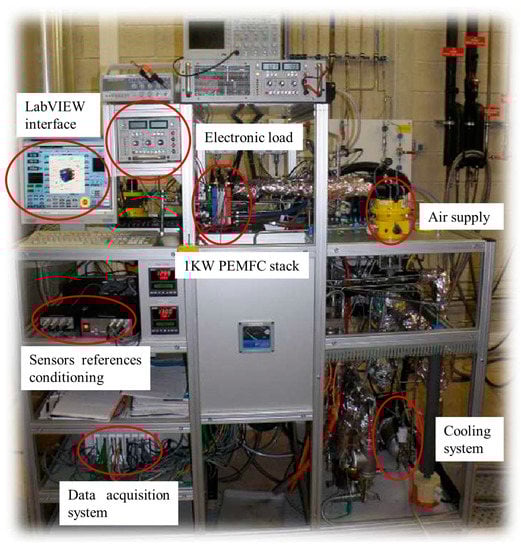
Figure 1.
PEMFC system experimental platform [34].
Since the raw voltage data contains a lot of noise and spike, the data needed to be preprocessed. The singular spectrum analysis (SSA) method can well extract the trend, periodic, and noise signals from the fuel cell voltage [31]. Therefore, the raw data were denoised by SSA in this paper. The detailed steps of SSA [31] are as follows:
Suppose the raw PEMFC degradation voltage series is , and is the window length. The L-lagged vectors can be defined as . The trajectory matrix can be obtained:
is the covariance matrix and . The singular value decomposition (SVD) is used to produce the eigenvalue and eigenvector . Let , and ; the SVD of can be described as follows:
Assuming that a group of indices , is described as , the trajectory matrix is .
Let be a matrix, , , and set ; else . Diagonal averaging transfers matrix into a series by Equation (3):
In addition, since the voltage sequence denoised by SSA still contains more than 140,000 data points, it will take a lot of time to process and calculate. Therefore, the denoised voltage sequence was resampled at an interval of 1 h, to obtain a reconstructed voltage sequence containing 1155 data. The preprocessed voltage data are shown in Figure 2.
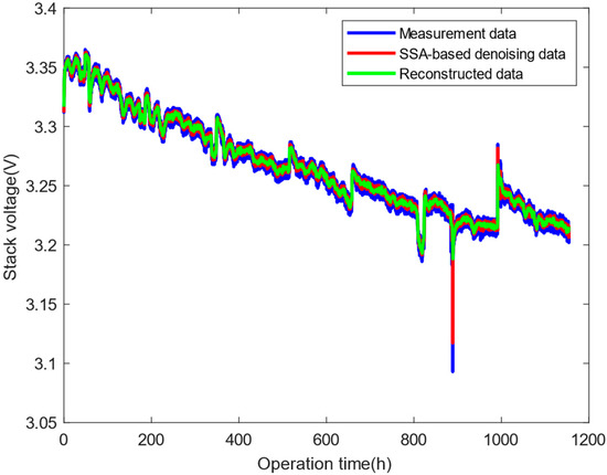
Figure 2.
The SSA denoised voltage sequence.
3. Methodology
3.1. LSTM Architecture
As a special type of recurrent neural network (RNN), LSTM has the ability to avoid the long-term dependency. Thus, the ability to remember information for a long time is inherent in LSTM. The architecture of LSTM is shown in Figure 3. LSTM has two memory states, the hidden state () and the cell state (). The memory states of LSTM are controlled by three types of gates, namely the input gate , the forget gate , and the output gate . The expressions of LSTM [21] are as follows.
where is the input sequence at the current moment, and and denote the current and previous outputs of hidden state, respectively. and denote the memory cell state of the current and previous moment, respectively. , , , and represent weights matrixes, and , , , and represent the bias vectors. represents the sigmoid function, and is the hyperbolic tangent function.
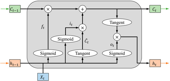
Figure 3.
LSTM architecture.
The fundamental procedure of LSTM is as follows. First, the LSTM determines what information in the cell state is supposed to be retained or forgotten, which is decided by the forget gate. Then, the hidden state of the last LSTM cell and the current input are taken to determine the information that needs to be stored in the cell state. After the current cell state is acquired, the hidden state can be calculated by using the cell state and the current input.
3.2. Gaussian Process Regression
GPR is a probabilistic prediction algorithm based on statistical learning and Bayesian theory [35,36]. For a given training dataset , where is the dimensional input vector, is the dimensional input matrix, is the corresponding output scalar, and is the output vector, a simple regression model can be described as [36]:
where is the observation contaminated by additive noise, is the input vector of the training set, and denotes the functional relationship. Suppose is a Gaussian distributed noise with variance of , . Then, the prior distribution of the observation can be derived.
Based on Bayesian principle, the joint Gaussian distribution of the predicted output and the observation y is obtained.
where is the kernel function, and is the n-dimensional identity matrix. The kernel function denotes the symmetric positive definite covariance matrix for computing the covariance of the training set itself. Similarly, the covariance of the test set itself and the covariance between and can be calculated by and , respectively. Then, based on the Bayesian framework, the posterior distribution of the predicted value can be obtained.
where is the predicted value of the test set data calculated by the Gaussian process regression model, and is the variance corresponding to the predicted value.
Then, based on and , the 95% confidence interval of the predicted value can be obtained as [, ]. In this paper, Matern 5/2 was chosen as the kernel function, and the expression is as follows.
where and are the hyperparameters of the kernel function that can be obtained by maximizing the likelihood function during the training process.
3.3. Extend Kalman Filter
The semi-empirical degradation model [9] is shown below.
where is the stack voltage; is the open-circuit voltage; is the number of cells; is the total resistance of the stack; is the stack temperature; , , and are the stack current, the exchange current, and the limiting current, respectively; and A and B are the Tafel constant and the concentration constant, respectively. According to [9], and are chosen as time-varying parameters to depict the degradation phenomenon. In addition, the other initial parameters of the semi-empirical degradation model were acquired from [14].
where α denotes the degradation degree of the fuel cell, and β denotes the degradation rate which can be considered as constant. Thus, the degradation of the fuel cell voltage can be described as a nonlinear process as shown in Equation (21). Additionally, the observation equation of the model is shown in Equation (24).
where is the system aging state; and are the system input and output, respectively; and and denote the process noise and measurement noise, respectively. The process of the EKF algorithm [9] is illustrated in Table 1.

Table 1.
The process of the EKF.
3.4. The Novel Hybrid Method for PEMFC Prognosis
As mentioned above, in the short-term prognostic, most of the existing research only focuses on improving prediction accuracy, and the confidence degree of the prediction results is not considered. For long-term prognostics, the variation in measurement noise variance is not considered during the prediction phase in some hybrid methods. In this paper, a short- and long-term prognostic method for PEM fuel cells based on Gaussian process regression is proposed.
The novel hybrid performance degradation prediction method of PEMFC is shown in Figure 4, which consists of three main parts: the main flow of the fuel cell degradation prediction method, the short-term degradation prediction method based on LSTM-GPR, and the long-term degradation prediction method based on EKF-GPR.
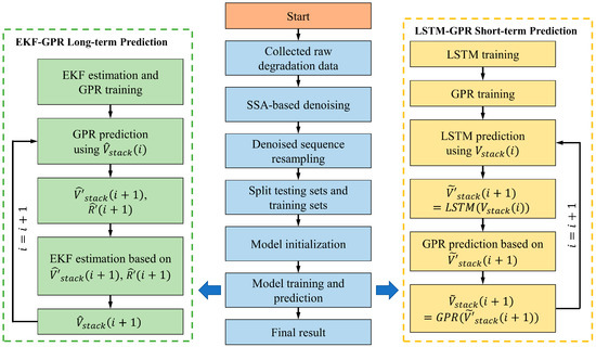
Figure 4.
The diagram of the hybrid performance degradation prediction method.
3.4.1. Short-Term Prediction Based on LSTM-GPR
The short-term prediction algorithm based on LSTM-GPR consists of a training phase and prediction phrase. During the training phases (TPs), the LSTM is first trained using the training set , where and are the input vectors and observations of the training set, respectively. Second, input the training set into the trained LSTM to obtain the prediction result . Then, use the training set to train the GPR to establish the relationship between the LSTM prediction results and the real voltage. During the prediction phase, LSTM predicts the next moment voltage based on the current moment voltage. Then, LSTM prediction results are fed to GPR for the second prediction. In Figure 4, , , and are the real fuel cell voltage, LSTM predicted voltage, and GPR predicted voltage, respectively. The training and prediction process of the LSTM-GPR method is shown in Algorithm 1.
| Algorithm 1: LSTM-GPR Method Algorithm |
| Split training sets and testing sets For j = 1:TP LSTM training using and Get LSTM network and prediction based on training sets End For j = 1:TP GPR training using and Get GPR network End For i = TP: length , , End Using the as the final prediction |
3.4.2. Long-Term Prediction Based on EKF-GPR
The long-term prediction algorithm based on EKF-GPR consists of a training phase and prediction phrase. During the TPs, the aging parameters are estimated by the EKF, and the fuel cell output voltage is used to train the GPR. During the prediction phase, the EKF estimates the stack voltage based on the voltage and variance predicted by the GPR. The estimation result of the EKF at the current moment is then sent to the GPR for the next prediction. In Figure 4, and are the fuel cell voltage and variance predicted by GPR, respectively, and is the voltage estimated by the EKF. The training and prediction process of EKF-GPR method is in Algorithm 2.
| Algorithm 2: EKF-GPR Method Algorithm |
| For j = 1:TP GPR training, EKF estimation Get and GPR network End For i = TP: length , Using as the observation of EKF, Using as the measurement noise variance of EKF Get End Using the as the final prediction |
4. Experimental Results and Discussion
For short-term degradation prediction, the performance of the prediction method can be evaluated by mean absolute error (MAE), mean absolute percentage error (MAPE), and root mean square error (RMSE). The evaluation criteria of prediction performance of PEMFC are defined as follows.
where is the number of voltage points in the test set, is the predicted voltage, and is the true stack voltage.
For long-term degradation prediction, assuming that the prediction starts at time , the predicted RUL is defined as the difference between the predicted end-of-life (EOL) time and the current time [37], as shown in the following equation.
4.1. Short-Term Prediction Results Based on LSTM-GPR
4.1.1. Performance Comparison of Different Prediction Methods
In order to verify the effectiveness of LSTM-GPR, the proposed hybrid model is compared with the individual models, namely the LSTM model and the GPR model. It should be noted that the LSTM model and GPR model are completely consistent with the corresponding parts in the hybrid model, respectively.
In the comparison experiments, all models are trained with the first 450 h of voltage data, and the employed training datasets are the voltage data that has been SSA denoised and resampled. In addition, each method makes predictions based on the voltage data one hour before the target moment. The single-step prediction results of the three methods are illustrated in Figure 5, and the prediction performance comparison is shown in Table 2.
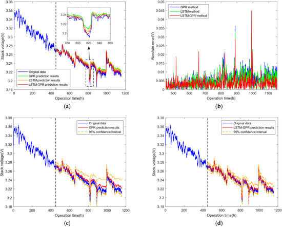
Figure 5.
Comparison of the prediction performance of the proposed LSTM-GPR method with the individual models: (a) voltage prediction results of the three methods; (b) absolute error of the three methods; (c) GPR prediction result; and (d) LSTM-GPR prediction results.
Table 2.
Comparison of the prediction results of the proposed method with individual model methods.
It can be seen from Figure 5a,b that all three methods can track the target voltage very well. The LSTM-GPR prediction model has a higher prediction accuracy than the other two models. As is seen in Table 2, all indicators of LSTM-GPR are better than the other two models. This is due to the deep structure formed by the combination of LSTM and GPR in the hybrid model, which has a stronger learning ability and can more accurately characterize the nonlinear details and the degradation trend of PEMFC.
By comparing Figure 5c,d, it can be seen that as the prediction time goes on, the voltage predicted by the GPR model will gradually deviate from the true voltage. Although the 95% confidence interval provided by the GPR model can cover most of the target voltage values, it will gradually increase with the prediction time, showing a divergence trend. Owing to the high-precision prediction of the LSTM network and the second prediction of the GPR, the predicted voltage curve of the LSTM-GPR model can better track the actual voltage curve, and the confidence interval can not only cover most of the target voltage but also has a more reliable distribution.
4.1.2. Performance Evaluation of LSTM-GPR with Different Sizes of Training Samples
The size of the training data has a significant impact on the performance of the degradation prediction model. The model is trained using the first 550 h, 650 h, 750 h, and 850 h aging voltage data as training data, respectively, to investigate the effect of the size of the training data in this section. The prediction results are illustrated in Figure 6. As can be seen, the size of the training data affects not only the prediction performance but also the distribution of the confidence interval. When the LSTM-GPR model is trained with more data, the prediction accuracy will be improved, and the distribution of its confidence interval will be more reliable.
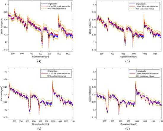
Figure 6.
LSTM-GPR model prediction performance with TP at: (a) 450 h; (b) 550 h; (c) 650 h; and (d) 750 h.
In order to verify the robustness of the LSTM-GPR method in PEMFC performance degradation prediction, the LSTM-GPR model is compared with DGP [31], which also has a deep structure at different TPs. The results are presented in Table 3; it can be seen that compared with DGP, LSTM-GPR has a higher accuracy at TPs of 450 h, 550 h, and 650 h. When TP is 750 h, both LSTM-GPR and DGP achieve a relatively high accuracy. Furthermore LSTM-GPR is less affected by the size of the training data.
Table 3.
Comparison of the prediction results of the proposed method with the DGP method at different training phases.
Based on the above analysis, it can be concluded that the proposed LSTM-GPR short-term degradation prediction model possesses advanced prediction performance and better robustness. Additionally, the method can not only predict the degradation details of PEMFC accurately but also provide reliable confidence intervals for the prediction results.
4.2. Long-Term Prediction Results Based on EKF-GPR
To verify the effectiveness of the EKF-GPR model in the long-term aging prediction of PEMFC, the model was trained using the first 600 h voltage data. According to [25], the voltage threshold of end-of-life was set to 3.5% of the initial voltage (Vinit = 3.345 V) of the fuel cell. Then its actual initial RUL is 792 h. The prognostics results of EKF-GPR at TP of 600 h are displayed in Figure 7. From Figure 7a, it can be seen that EKF-GPR can predict the degradation trend of fuel cell voltage very well. Additionally, the predicted RUL value is in good agreement with the actual data. In addition, it can be seen from Figure 7b that during the prediction stage, the measurement noise variance predicted by EKF-GPR is a divergent trend with the prediction time. It is because the prediction error will accumulate when there is no measured voltage data for model parameters updating during the prediction phase, resulting in the increase of the measurement noise variance. The experimental results show that the EKF-GPR method can achieve effectively RUL prediction.
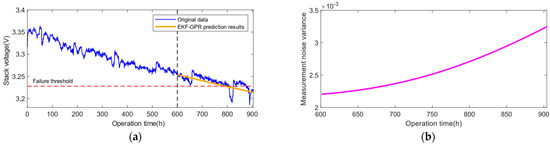
Figure 7.
Prediction results of the EKF-GPR approach at the TP of 600 h: (a)voltage prediction results and (b) measurement noise variance prediction results.
To test the accuracy and generality of the proposed method in RUL prediction, the proposed method is compared with EKF and GPR. The voltage prediction results of the three methods at different TPs (including 500 h, 550 h, 600 h, 650 h, 700 h, and 750 h) are depicted in Figure 8.
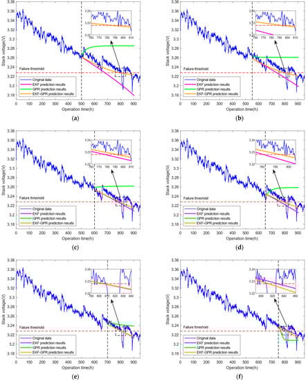
Figure 8.
Prediction performance of the EKF-GPR model at different training stages: (a) TP at 500 h; (b) TP at 550 h; (c) TP at 600 h; (d) TP at 650 h; (e) TP at 700 h; and (f) TP at 750 h.
As is shown in Figure 8, the prediction results of GPR model show a nonlinear trend but are far from the actual voltage data. Since there is no actual measurement data to update the model parameters, the prediction results of EKF show a linear trend. Therefore, the voltage degradation rate predicted by EKF is almost constant. It should be noted that the RUL prediction results of EKF at a TP greater than 600 h are more consistent with the actual RUL than that at a TP less than 600 h. It is because the prediction of EKF is based on the model parameters identified in the last step of TP, and its prediction performance is greatly affected by the status of the starting point. However, the EKF-GPR can predict the degradation trend very well at different TPs, thanks to its hybrid structure. The core idea of the EKF-GPR method is to use the predicted voltage of GPR as the observation of EKF and the predicted variance of GPR as the measurement noise variance of EKF. In addition, the input to GPR is the voltage filtered by EKF. Since GPR has good nonlinear prediction performance in the short term and can give reliable uncertainty, although the long-term prediction result of EKF is poor, it can also be improved by the prediction result of GPR.
Since the RUL prediction results of GPR are not available in most cases, this paper only presents the RUL prediction results of EKF and EKF-GPR methods, as shown in Figure 9. To obtain satisfactory results, the estimated RUL should be within the bounds ±10% of the true RUL. It can be seen from Figure 9 that most of the RULs estimated based on the EKF-GPR method are within the bounds ±10% of the actual RULs, and the prediction fluctuations are comparatively small. In contrast, the EKF method cannot guarantee the prediction accuracy at different TPs. Most of the estimated RULs of EKF are out of the bounds and fluctuate largely. The comparison results show that the proposed EKF-GPR method can achieve a more accurate RUL prediction.
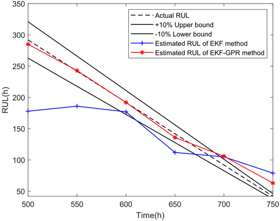
Figure 9.
Comparison of EKF-GPR method and EKF method of RUL prediction performance.
5. Conclusions
In this paper, a hybrid prognostic method is proposed to achieve short-term and long-term degradation predictions of PEMFC under stable operating conditions. The results showed that in the short-term prediction, the proposed LSTM-GPR method can extract depth degradation features from PEMFC degradation data due to its depth structure. This method effectively improves the short-term prediction accuracy and confidence interval reliability. Specifically, compared with the individual models (LSTM and GPR), the LSTM-GPR method could improve RMSE, MAE, and MAPE by at least 25.8%, 32.1%, and 38.9%, respectively. In comparison with DGP [31], which also has a deep structure, the average RMSE and MAE values of the LSTM-GPR method are reduced by nearly 13.7% and 18.2%, respectively. In the long-term prediction, the proposed EKF-GPR method has a higher accuracy compared with the EKF method and GPR method. Most of the RULs estimated by the EKF-GPR method are within the bounds ±10% of the actual RULs. However, the GPR method cannot obtain RUL prediction results in most cases, and the EKF method cannot guarantee the accuracy at different TPs. In summary, the proposed hybrid degradation prediction method has perfect performance in both short-term and long-term prognostics.
Nevertheless, there are also limitations in this study. Neither the short-term nor long-term prediction method takes into account variable load conditions. The adaptability of this method under complex operating conditions remains an issue. In addition, the PEMFC degradation mechanism has not been fully discovered, and how to construct an accurate PEMFC degradation model requires further research.
Author Contributions
Conceptualization, T.W.; Data curation, T.W. and C.Z.; Funding acquisition, H.Z.; Methodology, T.W.; Project administration, H.Z.; Software, C.Z.; Supervision, H.Z.; Validation, C.Z.; Writing—original draft, T.W.; Writing—review and editing, T.W. and H.Z. All authors have read and agreed to the published version of the manuscript.
Funding
This research was funded by the National Key R&D Program of China under the Grant No. 2018YFB1305402.
Institutional Review Board Statement
Not applicable.
Informed Consent Statement
Not applicable.
Data Availability Statement
Not applicable.
Conflicts of Interest
The authors declare no conflict of interest.
References
- Bahari, M.; Rostami, M.; Entezari, A.; Ghahremani, S.; Etminan, M. Performance evaluation and multi-objective optimization of a novel UAV propulsion system based on PEM fuel cell. Fuel 2022, 311, 122554. [Google Scholar] [CrossRef]
- Liu, H.; Chen, J.; Hissel, D.; Lu, J.; Hou, M.; Shao, Z. Prognostics methods and degradation indexes of proton exchange membrane fuel cells: A review. Renew. Sustain. Energy Rev. 2020, 123, 109721. [Google Scholar] [CrossRef]
- Eudy, L.; Post, M.B. Fuel Cell Buses in U.S. Transit Fleets: Current Status 2018; NREL: Golden, CO, USA, 2019. [Google Scholar]
- Das, V.; Padmanaban, S.; Venkitusamy, K.; Selvamuthukumaran, R.; Blaabjerg, F.; Siano, P. Recent advances and challenges of fuel cell based power system architectures and control—A review. Renew. Sustain. Energy Rev. 2017, 73, 10–18. [Google Scholar] [CrossRef]
- Yue, M.; Jemei, S.; Zerhouni, N.; Gouriveau, R. Proton exchange membrane fuel cell system prognostics and decision-making: Current status and perspectives. Renew. Energy 2021, 179, 2277–2294. [Google Scholar] [CrossRef]
- Sutharssan, T.; Montalvao, D.; Chen, Y.K.; Wang, W.-C.; Pisac, C.; Elemara, H. A review on prognostics and health monitoring of proton exchange membrane fuel cell. Renew. Sustain. Energy Rev. 2017, 75, 440–450. [Google Scholar] [CrossRef] [Green Version]
- Jouin, M.; Gouriveau, R.; Hissel, D.; Péra, M.-C.; Zerhouni, N. Prognostics and Health Management of PEMFC—State of the art and remaining challenges. Int. J. Hydrogen Energy 2013, 38, 15307–15317. [Google Scholar] [CrossRef] [Green Version]
- Jouin, M.; Gouriveau, R.; Hissel, D.; Péra, M.-C.; Zerhouni, N. Prognostics of PEM fuel cell in a particle filtering framework. Int. J. Hydrogen Energy 2014, 39, 481–494. [Google Scholar] [CrossRef] [Green Version]
- Bressel, M.; Hilairet, M.; Hissel, D.; Ould Bouamama, B. Extended Kalman Filter for prognostic of Proton Exchange Membrane Fuel Cell. Appl. Energy 2016, 164, 220–227. [Google Scholar] [CrossRef]
- Chen, J.; Zhou, D.; Lyu, C.; Lu, C. A novel health indicator for PEMFC state of health estimation and remaining useful life prediction. Int. J. Hydrogen Energy 2017, 42, 20230–20238. [Google Scholar] [CrossRef]
- Chen, K.; Laghrouche, S.; Djerdir, A. Fuel cell health prognosis using Unscented Kalman Filter: Postal fuel cell electric vehicles case study. Int. J. Hydrogen Energy 2019, 44, 1930–1939. [Google Scholar] [CrossRef]
- Zhang, D.; Baraldi, P.; Cadet, C.; Yousfi-Steiner, N.; Bérenguer, C.; Zio, E. An ensemble of models for integrating dependent sources of information for the prognosis of the remaining useful life of Proton Exchange Membrane Fuel Cells. Mech. Syst. Signal Process. 2019, 124, 479–501. [Google Scholar] [CrossRef] [Green Version]
- Ao, Y.; Laghrouche, S.; Depernet, D.; Chen, K. Proton Exchange Membrane Fuel Cell Prognosis Based on Frequency-Domain Kalman Filter. IEEE Trans. Transp. Electrif. 2021, 7, 2332–2343. [Google Scholar] [CrossRef]
- Pan, R.; Yang, D.; Wang, Y.; Chen, Z. Performance degradation prediction of proton exchange membrane fuel cell using a hybrid prognostic approach. Int. J. Hydrogen Energy 2020, 45, 30994–31008. [Google Scholar] [CrossRef]
- Ma, R.; Xie, R.; Xu, L.; Huangfu, Y.; Li, Y. A Hybrid Prognostic Method for PEMFC With Aging Parameter Prediction. IEEE Trans. Transp. Electrif. 2021, 7, 2318–2331. [Google Scholar] [CrossRef]
- Silva, R.E.; Gouriveau, R.; Jemeï, S.; Hissel, D.; Boulon, L.; Agbossou, K.; Yousfi Steiner, N. Proton exchange membrane fuel cell degradation prediction based on Adaptive Neuro-Fuzzy Inference Systems. Int. J. Hydrogen Energy 2014, 39, 11128–11144. [Google Scholar] [CrossRef] [Green Version]
- Hua, Z.; Zheng, Z.; Péra, M.-C.; Gao, F. Remaining useful life prediction of PEMFC systems based on the multi-input echo state network. Appl. Energy 2020, 265, 114791. [Google Scholar] [CrossRef]
- Ma, R.; Breaz, E.; Liu, C.; Bai, H.; Briois, P.; Gao, F. Data-driven Prognostics for PEM Fuel Cell Degradation by Long Short-Term Memory Network. In Proceedings of the 2018 IEEE Transportation Electrification Conference and Expo (ITEC), Long Beach, CA, USA, 13–15 June 2018; pp. 102–107. [Google Scholar]
- Ma, R.; Yang, T.; Breaz, E.; Li, Z.; Briois, P.; Gao, F. Data-driven proton exchange membrane fuel cell degradation predication through deep learning method. Appl. Energy 2018, 231, 102–115. [Google Scholar] [CrossRef]
- Zhu, L.; Chen, J. Prognostics of PEM fuel cells based on Gaussian process state space models. Energy 2018, 149, 63–73. [Google Scholar] [CrossRef]
- Liu, J.; Li, Q.; Chen, W.; Yan, Y.; Qiu, Y.; Cao, T. Remaining useful life prediction of PEMFC based on long short-term memory recurrent neural networks. Int. J. Hydrogen Energy 2019, 44, 5470–5480. [Google Scholar] [CrossRef]
- Liu, J.; Li, Q.; Han, Y.; Zhang, G.; Meng, X.; Yu, J.; Chen, W. PEMFC Residual Life Prediction Using Sparse Autoencoder-Based Deep Neural Network. IEEE Trans. Transp. Electrif. 2019, 5, 1279–1293. [Google Scholar] [CrossRef]
- Ma, R.; Li, Z.; Breaz, E.; Liu, C.; Bai, H.; Briois, P.; Gao, F. Data-Fusion Prognostics of Proton Exchange Membrane Fuel Cell Degradation. IEEE Trans. Ind. Appl. 2019, 55, 4321–4331. [Google Scholar] [CrossRef]
- Wang, F.-K.; Cheng, X.-B.; Hsiao, K.-C. Stacked long short-term memory model for proton exchange membrane fuel cell systems degradation. J. Power Sources 2020, 448, 227591. [Google Scholar] [CrossRef]
- Zhang, Z.; Wang, Y.-X.; He, H.; Sun, F. A short- and long-term prognostic associating with remaining useful life estimation for proton exchange membrane fuel cell. Appl. Energy 2021, 304, 117841. [Google Scholar] [CrossRef]
- Wang, C.; Li, Z.; Outbib, R.; Dou, M.; Zhao, D. A novel long short-term memory networks-based data-driven prognostic strategy for proton exchange membrane fuel cells. Int. J. Hydrogen Energy 2022, 47, 10395–10408. [Google Scholar] [CrossRef]
- Meiling, Y.; Zhongliang, L.; Robin, R.; Samir, J.; Noureddine, Z. Degradation identification and prognostics of proton exchange membrane fuel cell under dynamic load. Control Eng. Pract. 2022, 118, 104959. [Google Scholar]
- Benaggoune, K.; Yue, M.; Jemei, S.; Zerhouni, N. A data-driven method for multi-step-ahead prediction and long-term prognostics of proton exchange membrane fuel cell. Appl. Energy 2022, 313, 118835. [Google Scholar] [CrossRef]
- Cheng, Y.; Zerhouni, N.; Lu, C. A hybrid remaining useful life prognostic method for proton exchange membrane fuel cell. Int. J. Hydrogen Energy 2018, 43, 12314–12327. [Google Scholar] [CrossRef]
- Xie, R.; Ma, R.; Pu, S.; Xu, L.; Zhao, D.; Huangfu, Y. Prognostic for fuel cell based on particle filter and recurrent neural network fusion structure. Energy AI 2020, 2, 100017. [Google Scholar] [CrossRef]
- Xie, Y.; Zou, J.; Peng, C.; Zhu, Y.; Gao, F. A novel PEM fuel cell remaining useful life prediction method based on singular spectrum analysis and deep Gaussian processes. Int. J. Hydrogen Energy 2020, 45, 30942–30956. [Google Scholar] [CrossRef]
- Wang, Y.; Feng, B.; Hua, Q.-S.; Sun, L. Short-Term Solar Power Forecasting: A Combined Long Short-Term Memory and Gaussian Process Regression Method. Sustainability 2021, 13, 3665. [Google Scholar] [CrossRef]
- Sheng, H.; Xiao, J.; Wang, P. Lithium Iron Phosphate Battery Electric Vehicle State-of-Charge Estimation Based on Evolutionary Gaussian Mixture Regression. IEEE Trans. Ind. Electron. 2017, 64, 544–551. [Google Scholar] [CrossRef]
- Fabien Harel (2021): IEEE PHM Data Challenge 2014. Fuel Cell Lab (UAR 2200). Available online: https://dataosu.obs-besancon.fr/FR-18008901306731-2021-07-19_IEEE-PHM-Data-Challenge-2014.html (accessed on 3 May 2022).
- Kang, L.; Chen, R.S.; Xiong, N.; Chen, Y.C.; Hu, Y.X.; Chen, C.M. Selecting Hyper-Parameters of Gaussian Process Regression Based on Non-Inertial Particle Swarm Optimization in Internet of Things. IEEE Access 2019, 7, 59504–59513. [Google Scholar] [CrossRef]
- Rasmussen, C.E.; Williams, C.K.I. Gaussian Processes for Machine Learning; The MIT Press: Cambridge, MA, USA, 2005. [Google Scholar]
- Chen, K.; Laghrouche, S.; Djerdir, A. Health state prognostic of fuel cell based on wavelet neural network and cuckoo search algorithm. ISA Trans. 2021, 113, 175–184. [Google Scholar] [CrossRef] [PubMed]
Publisher’s Note: MDPI stays neutral with regard to jurisdictional claims in published maps and institutional affiliations. |
© 2022 by the authors. Licensee MDPI, Basel, Switzerland. This article is an open access article distributed under the terms and conditions of the Creative Commons Attribution (CC BY) license (https://creativecommons.org/licenses/by/4.0/).