Abstract
The increasing Photovoltaic (PV) penetration in residential Low Voltage (LV) networks is likely to result in a voltage rise problem. One of the potential solutions to deal with this problem is to adopt a distribution transformer fitted with an On-Load Tap Changer (OLTC). The control of the OLTC in response to local measurements reduces the need for expensive communication channels and remote measuring devices. However, this requires developing an advanced decision-making algorithm to estimate the existence of voltage issues and define the best set point of the OLTC. This paper presents a decentralized data-driven control approach to operate the OLTC using local measurements at a distribution transformer (i.e., active power and voltage at the secondary side of the transformer). To do so, Monte Carlo simulations are utilized offline to produce a comprehensive dataset of power flows throughout the distribution transformer and customers’ voltages for different PV penetrations. By the application of the curve-fitting technique to the resulting dataset, models to estimate the maximum and the minimum customers’ voltages are defined and embedded into the control logic to manage the OLTC in real time. The application of the approach to a real UK LV feeder shows its effectiveness in improving PV hosting capacity without the need for remote monitoring elements.
1. Introduction
1.1. Background
In the last decade, different energy policies have been introduced to encourage the uptake of residential solar Photovoltaics (PV) as a crucial step to facilitate the transition toward low-carbon energy systems [1]. For instance, the net-metering and the feed-in tariff schemes adopted in different countries provide significant incentives to support PV installations [2]. However, the rapid growth in residential PV capacities has placed technical impacts on distribution networks, particularly at the Low Voltage (LV) networks [3]. This, in particular, during time intervals with high PV generation and minimum demand. The excess PV generation flowing back to the upstream grid (i.e., reverse power flow) may cause voltage rise issues above the allowed voltage range [4]. To mitigate the PV impacts, Distribution Network Operators (DNOs) adopt conservative PV connection rules to restrict the maximum PV capacity connected to a LV feeder [5].
The technological advancements in PV inverters enable actively managing customers’ voltages by controlling excess PV generation below a defined export limit [6,7,8,9]. However, this may result in an unnecessarily large volume of energy curtailment with the adoption of a relatively small export limit to cater to the worst-case scenario of maximum generation and minimum demand. Further, this approach requires amending the existing regulatory rules to allow the application of PV curtailment.
Alternative DNO-based control solutions are needed to accelerate the uptake of residential PV systems [10,11,12]. One of the potential solutions is to reduce voltages at the LV busbar of distribution transformers to allow additional headroom of voltage rise at customers’ connection points [13]. In particular, a larger volume of voltage reduction is required at high PV penetrations to mitigate the PV impacts [14]. Thus, it is necessary to read just the LV busbar voltage during evening and nighttime periods to prevent voltage drop issues when there is the peak demand of residential feeders [15]. However, the frequent daily voltage changes cannot be directly implemented in practice with the conventional distribution transformers equipped with off-load tap changers since load disconnections are needed to modify the tap position [16]. In addition, the limited voltage capability range of the off-load tap changer (e.g., ±5%) may not be sufficient to mitigate voltage issues taking into account that the ratios of distribution transformers are normally designed to provide voltage gain above the rated voltage (e.g., 3.75% voltage boost at the nominal tap position) [17].
1.2. Literature Review
To cater for the above challenges, distribution transformers could be equipped with an on-load tap changer (OLTC) to automatically regulate LV busbar voltages and mitigate PV impacts [18,19]. In the literature, the employment of OLTCs in LV networks has been extensively studied particularly from the control perspective.
Most of the studies in the literature consider managing the operations of OLTCs using optimization-based approaches. These studies demonstrate the effectiveness of Optimal Power Flow (OPF) to manage LV constraints through the optimal control of OLTCs and other network controllable elements such as PV inverters, switching elements, and capacitor banks [20,21,22]. Nonetheless, the implementation of OPF-based control approaches in practice is challenging. To drive the OPF with real-time voltage and power measurements, a significant number of monitoring elements are needed at both customers’ connection points and throughout LV feeders. Further, extensive communication infrastructure is required to track the changes in voltages and power measurements.
Alternative rule-based control approaches are proposed in [23,24]. To define the best set points of OLTCs, remote voltage measurements are placed at critical locations whose voltages are the maximum ones in the network. However, the locations of maximum voltage might not be the same for all PV penetrations. Thus, it is still needed to increase remote measurement elements with the evolution of PV penetration.
Advanced local voltage control approaches are proposed in [25,26] to estimate maximum network voltages based only on local measurements at the distribution transformer without the need for remote monitoring elements. However, complex algorithms are adopted to drive the control logic such as estimating the number of customers, topology, and impedances of LV feeders. In addition, multiple parameters have to be properly defined and fine-tuned. Alternatively, the rolling out of smart meters along with the efforts to produce readily available data of LV feeders in recent years provide a significant volume of data that could be harnessed to facilitate the development of simpler and more implementable voltage control approaches.
To implement the OLTC control approach in practice, it is important, first, to assess, using simulations, its effectiveness to solve voltage issues under different network operating conditions. In addition, the impacts of the real-time operational aspects on the number of tap changes have to be adequately quantified. To do so, Monte Carlo simulations have been adopted in the literature to cater to uncertainties in demand and PV [27,28]. However, the scenarios covered in the Monte Carlo simulations are randomly produced without properly and securely capturing the most-critical and effective scenarios.
1.3. Research Gap with Novelty
To adequately address the aforementioned emerging challenges and bridge the gaps that have arisen in the literature, this work proposes a new data-driven-based control approach to manage the operation of OLTCs in residential LV networks with high PV penetration. The optimal set points of OLTCs are found using local measurements at the distribution transformer (i.e., active power and voltage at the secondary side of the transformer). For this purpose, block-based Monte Carlo simulations are utilized to produce an ‘off-line’ full dataset of the potential combinations of power flows at the distribution transformer and the customers’ voltages. The dataset is also produced considering different values of LV busbar voltage. By the application of the curve-fitting technique to the resulting dataset, mathematical models of the estimated customers’ voltages are defined. The resulting models are embedded in the control logic to produce the best set point of the OLTC to solve voltage rise problems whilst keeping voltages at demand-led LV feeders above the lower statutory limit. The control approach is applied to a real UK underground residential LV network. The performance of the proposed approach is investigated considering different control cycles, in particular, the number of tap operations and the compliance of voltages with the allowed voltage range in the EN50160 standard (applied in the UK).
This paper is structured as follows: Section 2 presents an overview of the voltage control approach. The formulations are given in Section 3. In Section 4 and Section 5, the results from the application of the approach on a UK residential LV network with PV are presented and discussed. Conclusions are drawn in Section 6.
2. Overview
The aim of the proposed approach is to manage voltages in LV networks using OLTCs without the need for remote monitoring elements. To do so, it is important to develop mathematical models that allow estimating customers’ voltages in real time according to the available local measurements at the distribution transformer. This includes measurements related to the active and reactive power measurements at the distribution transformer and the voltage at the secondary side of the transformer (LV busbar voltage). The adequate definition of the mathematical model requires capturing the type of relationships (e.g., linear, non-linear) between customers’ voltages and the available local measurements. In addition, the sensitivities of customers’ voltages to the changes in each individual measurement have to be extracted and expressed as the model coefficients. To do so, a large volume of readily available data is needed. For this purpose, a block-matrix-based Monte Carlo approach is adopted to produce the dataset. It was produced by performing multiple three-phase unbalanced power flow simulations that are carried out to cover the potential combinations of PV locations and sizes as well as PV generation and customers’ load profiles. Further, the simulations are carried out considering different values of LV busbar voltage. For each power flow simulation, the maximum and minimum customers’ voltages are registered along with the corresponding power flows at the distribution transformer. By the application of the curve-fitting technique to the resulting dataset, the mathematical models required to estimate customers’ voltages are defined. The resulting models are embedded in the control logic to estimate the maximum and minimum customers’ voltages to define the best set point of OLTC.
To demonstrate the proposed approach to control OLTC, Figure 1 presents graphically an example of the mathematical models to estimate maximum voltage in the network (the vertical axis) based on the active power flows at the distribution transformer (the horizontal axis). Multiple curves are also presented. Each of them corresponds to a particular value of LV busbar voltage (Vreg). The upper curve (red line) is the one with the highest target voltage (Vreg1). It can be seen that the maximum voltage increases linearly with higher levels of export power at the distribution transformer (i.e., negative values of active power flows). It can be noticed that it is possible to estimate the occurrence of a voltage rise problem based on the intensity of export power. With a busbar voltage of Vreg2 (green line), for instance, it can be expected that one of the customers (at the least) receives voltage beyond the upper statutory limit (Vmax) when the absolute value of export power exceeds P2. Once the control approach detects the existence of voltage issues, the LV busbar voltage has to be updated. Let us assume that the reverse power flow throughout the transformer is P3 while the LV busbar is set to Vreg2. This means that there is a voltage rise problem in the network. By adjusting (reducing) the target voltage of the OLTC to Vreg3 (blue line), it is possible to bring back customers’ voltages within limits. Before updating the target voltage to Vreg3, it is important to check whether it may cause voltage drop issues at demand-led LV feeders. This is performed by estimating the minimum voltage in the network using the corresponding offline defined mathematical models. Thus, the best LV busbar voltage is selected to maintain customers’ voltages within the upper and the lower limits. The control logic continues monitoring power flows throughout each control cycle (e.g., every five minutes) of the transformer to estimate customers’ voltages and update the OLTC’s set point.
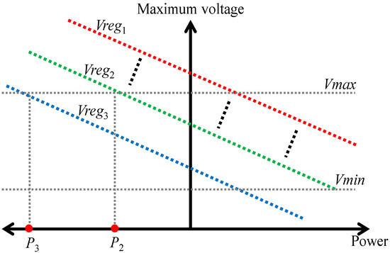
Figure 1.
A graphical example of the relationships between the power at the distribution transformer and the maximum voltage at residential customers for different LV busbar voltage.
3. Methodology
This section presents the details and the formulations of the methodology to manage voltages in LV networks. The methodology encompasses the planning stage to produce offline the best models to estimate voltages. The operational stage to control the OLTC in real time is then provided.
3.1. Planning Stage
The model to estimate voltages in LV networks is defined in a two-step process. First, a Monte Carlo-based approach is adopted to generate the dataset required to extract the coefficients. Then, a curve-fitting approach is utilized to produce the coefficients of the model.
3.1.1. Dataset Generation “Block-Matrix Monte Carlo Approach”
The estimation of customers’ voltages according to the intensities and directions of power flows at the distribution transformer requires identifying properly the values of critical power flows that indicate the possible occurrence of voltage issues. The inadequate definition of critical power flows may not allow identifying the existence of voltage issues. However, this is a challenging task for the decision-making algorithm considering there is limited/no available information about the locations and sizes of PV systems as well as the load data in the LV network. In particular, the impacts of a specific PV penetration on network voltages depend on the particular combinations of PV and demand data. To cater for these challenges, the first process in the planning stage aims to assess offline the effects of the possible combinations of individual customers’ net demand on the operating conditions of the LV network. The resulting dataset of power flows at the distribution transformer, and customers’ network voltages will be then utilized to support the operation of the voltage control logic. To ensure the spectrum of operating conditions is covered, the block-matrix-based Monte Carlo approach is adopted.
The block-matrix-based Monte Carlo approach assesses the network operating conditions for M number of PV penetration. At each PV penetration, N number of scenarios of PV locations are considered. The allocation of PV is performed to ensure unique combinations of PV locations. To realistically model the PV growth, such as in real-life LV networks, the scenarios are also coupled throughout PV penetrations. In a specific scenario, the transition from a PV penetration to the next higher one is carried out by placing new PV locations next to those from the previous penetration. The number of PV locations is increased progressively throughout PV penetrations until a single PV is placed at each customer (i.e., 100% PV penetration). The PV sizes could be determined according to national statistics for residential rooftop PV deployment. In a specific scenario, the customers’ PV sizes at a lower PV penetration are also maintained the same as at higher penetration. Further, the tool developed by the Centre for Renewable Energy Systems Technology (CREST) model is used to produce daily and seasonal residential load profiles [29]. The resulting profiles are distributed among customers to satisfy national statistics related to the number of residents per house. A single normalized PV power profile is also adopted for all the residential customers with PVs. The PV profile is selected from a set of representative normalized PV power generation profiles (adopted from [30]). For each scenario per PV penetration, three-phase 4-wire daily power flow simulations are performed to calculate network voltages and power flows for each of the representative PV profiles. Further, the power flow simulations will be carried out at each scenario considering different LV busbar voltages.
It is worth highlighting that the definition of scenarios before performing the power flows simulations provides identical platforms to compare control methods with different control cycles and realistically quantifies the improvement brought from the potential solutions employed. Further, the adopted Monte Carlo approach provides contributions from previous approaches in the literature that produce scenarios by simply randomizing PV generation and load data. This facilitates dealing with the uncertainties and the complexity brought from multiple stochastic parameters (e.g., demands, PV sizes and locations) to assess the PV hosting capacity. In addition, the Monte Carlo approach supports identifying the potential risk of voltage violations at each PV penetration and control cycle. The risk corresponds to the frequency of scenarios per PV penetration whose customers’ voltages are outside the voltage limits. In practice, this enables DNOs to adequately determine the PV hosting capacity within a predefined and acceptable risk level.
To demonstrate mathematically the concept of block matrix, the following matrices are defined for a given scenario (set SC indexed by sc) at a PV penetration (set Pent indexed by pent). First, a matrix is defined in Equation (1) to represent the PV locations across K number of residential customers. Its elements are either 1 or 0 (i.e., binary values) to indicate the PV locations (e.g., means that a PV system is assigned to the first customer). Similarly, the matrix in Equation (2) represents the residential PV ratings. This matrix has one row and K columns to represent the PV rating per customer. The demand profiles for the K number of residential customers across a day with T time steps are given in Equation (3). Each column in the matrix corresponds to the daily demand profile per residential customer. For instance, the parameters to indicate the values of daily demand profile for the first customer. Further, the () matrix in Equation (4) indicates the normalized daily PV power profiles per each residential customer with a dimension of T × K.
The above matrices in Equations (1)–(4) are all concatenated vertically to produce the block matrix in Equation (5) with 2T + 2 rows and K columns for the scenario sc and penetration pent.
Once the block matrices are produced for all the scenarios and PV penetration, as formulated in Equation (6), three-phase power flows are carried out to assess the network operating conditions in response to the generation and demand data per each block matrix. In addition, the power flows are repeated for different values of LV busbar voltage (). Based on the power flow data, the mean active and reactive power flows throughout the transformer, the daily customers’ maximum, and minimum voltages are all extracted and registered in the matrices , , and Equations (7)–(10), respectively. These matrices will be then used in the second process of the planning stage to produce the mathematical models required to estimate network voltages.
3.1.2. Voltage Estimation Models “Curve-Fitting Approach”
Here, it is aimed to produce the mathematical functions that express the relationships between customers’ voltages and the active and reactive power throughout the distribution transformer. The resulting functions will be then embedded in the real-time voltage control scheme to manage the voltages. By using the curve-fitting technique, a single function will be defined per each PV penetration and LV busbar voltage. The best-fitted curves will be extracted from the network operating conditions found in the first process of the planning stage whose values are registered in the matrices Equations (7)–(10). For instance, the active and reactive power flows across the N scenarios of the first PV penetration, i.e., the first columns of the matrices in Equations (7) and (8), and the corresponding customers’ maximum voltage, i.e., the first column of the matrix in Equation (9), will be all input to the curve-fitting technique to define the function to predict customers’ maximum voltages at the first PV penetration. In addition, the function to estimate the minimum customers’ voltages at the first PV penetration will be defined according to the data points in the first columns of the matrices Equations (7), (8), and (10). The curves to predict maximum and minimum customers’ voltages () at a LV busbar voltage () are mathematically given in Equations (11) and (12), respectively.
where () are the active and reactive power measurements at the distribution transformer.
To perform the curve fitting technique, it is also required to define the shapes of the curves (e.g., linear). Taking into account the high ratios of resistance to the reactance of LV lines (i.e., R >> X) and the relatively very small changes in voltage phase angles in LV networks, linear relationships are adopted. Thus, it is assumed that the customers’ voltages are linearly varied according to the changes in the power measurements at the distribution transformer. The functions to estimate customers’ maximum and minimum voltages are formulated in Equations (13) and (14), respectively. It is worth highlighting that the functions are also produced for different values of LV busbar voltages.
The functions express the maximum and minimum voltages according to the values of active and reactive power throughout the transformer (two terms). However, it may not be possible to produce a curve that perfectly passes throughout all the data points. There could be some variations between the data points and the fitted curves (i.e., residual errors). Thus, for each function, the curve-fitting technique aims to minimize the sum of squared distances from the data points to the fitted curve (i.e., least square) by estimating the best values for the three coefficients ( and and coefficients). The coefficient represents the estimated customers’ maximum voltage when the active and reactive power equal zero (i.e., no-load condition). Thus, the value of the coefficient is equal to the LV busbar voltage. The adoption of higher values of LV busbar voltage increases both the customers’ voltage and the coefficients. In contrast, the and coefficients represent how well the active and reactive power throughout the transformers can predict the variations in the customers’ voltages. Due to the technical characteristics of LV networks, it is expected that the changes in the reactive power throughout the transformer would have little effect on predicting customers’ voltages and making the sum of squared error smaller. Thus, it is likely that the curve fitting will result in small values of coefficients. Therefore, a linear equation is anticipated between the active power flow throughout the transformer and customers’ voltages. However, it is important to measure mathematically the strength of the linear relationship between both variables. This is performed by identifying the values of the correlation coefficients (). Higher absolute values of the correlation coefficient (i.e., close to unity) indicate the existence of strong linear relationships. It is also important to highlight that the sign of the correlation coefficient represents the direction of relationships (e.g., −1 indicates strong negative relationships). To further improve the estimation models, other statistical-based correlation coefficients could be explored to identify the existence and the strength of the relationship (linear or non-linear) between customers’ voltages and other different parameters such as ambient temperature and irradiance. For instance, the Spearman rank-order correlation coefficient can be adopted to assess the correlation.
3.2. Operational Stage “Control Logic of OLTC”
This section provides a description of the proposed control logic of the OLTC to manage voltages in LV distribution networks. Typically, the OLTC is fitted at the high voltage side of the distribution transformer. By using an automatic voltage control relay, the tap ratio of the OLTC is automatically adjusted to regulate the voltage at the LV busbar of the distribution transformer close to a predefined desired target voltage (). When the measured voltage at the LV busbar () is outside the allowed voltage tolerance (e.g., bandwidth) for consecutive time steps (e.g., 2 min), the control logic is triggered to change the tap position. The required number of tap changes is determined according to the voltage difference between the measured LV busbar voltage and the desired target voltage. Thus, the selection of the target voltage is crucial to ensure the effective voltage management of customers’ voltages within their allowed upper and lower limits (). Taking into account that the proposed voltage management approach is communication-free (without remote monitoring elements), customers’ maximum and minimum voltages () have to be predicted in real time. For this purpose, the functions developed in Equations (13) and (14) are considered by the control logic to guess customers’ voltages according to the real-time active and reactive power measurements throughout the transformer (,) and the voltage of LV busbar (). This means that the desired target voltage keeps adjusting in real-time according to the estimated customers’ maximum and minimum voltages. The proposed control logic is shown in Figure 2. The control logic aims to adjust the target voltage from its current value () by n discrete number of voltage step such that the estimated customers’ maximum and minimum voltages are kept within their limits. Each voltage step corresponds to the voltage change per one tap change. Due to the voltage capabilities of OLTC, the new target voltage has to be kept between its minimum and maximum values (, ).
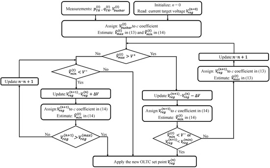
Figure 2.
Flow chart of the operational stage.
The control logic shows in detail the process to define the updated target voltage. Once the voltage estimation indicates the existence of customers’ voltage violations, an iterative approach is performed to select the best setting of the target voltage. At each iteration n, the target voltage is decreased by from its previous value. The corresponding effect on the customers’ maximum voltage is checked by updating the coefficients in Equation (13). This process is continued until either the maximum voltage capability of OLTC to reduce voltage is achieved () or the estimated customers’ minimum voltages according to Equation (14) falls below its lowest limit (). A similar process is also adopted to cater for voltage drop issues such that the target voltage is increased in fixed steps throughout the iterations until the estimated customers’ minimum voltages are above its statutory limit. Once the new voltage set point is identified, it is sent to the OLTC and implemented throughout the next control cycle. In response to the new set point, the automatic voltage control relay sends raise or lower tap position commands. It is worth highlighting that different control cycles (e.g., 10 min) could be adopted. The most adequate control cycle is a trade-off between the effectiveness to manage voltage constraints and the number of tap changes. Further, it is important to highlight that the control logic takes into account the existing PV penetration to properly select the coefficients of functions in Equations (13) and (14).
4. Results: Case Study
In this section, the methodology described in Section 3 is applied to a real underground residential LV network considering demand and PV generation profiles. Realistic PV impact analysis is, later, carried out considering 11 PV penetration (from 0 to 100 with an increment of 10%). The benefits to improve PV hosting capacity are then demonstrated. All the corresponding results are presented.
4.1. Real UK LV Network
The proposed approach is applied to a real underground residential LV network (located in the North West of England) [31]. The network (11 kV/415 V) consists of six radially operated feeders (each one is three phases and four-wire cables). A single-line schematic of the studied network is shown in Figure 3 on which the triangle shape represents the distribution transformer (rated capacity 500 kVA). The LV Feeders are presented with different colors. All customers are with single-phase connections. For this purpose, the distribution network analysis software package OpenDSS is utilized to perform time-series and three-phase unbalanced power flows [32].
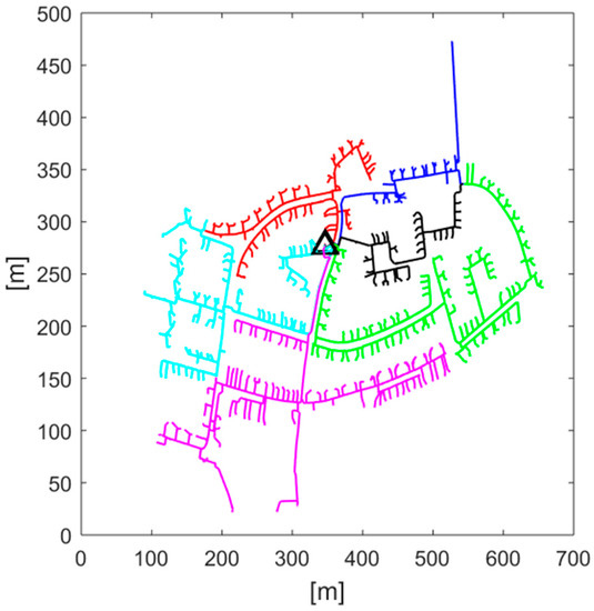
Figure 3.
Schematic for the studied network with six LV Feeders (each LV feeder is presented with different color).
4.2. Demand and PV Generation Profiles
The tool provided by the Centre for Renewable Energy Systems Technology (CREST) in [29] is employed for modeling/producing the residential profiles considering the one-minute resolution. Each load of household is realistically modeled taking into account type of day, seasonality, number of occupancies, and the corresponding usage of electrical appliances. For the studied network, the adopted number of residents per dwelling aligns with UK statistics. For the PV systems, the same day is selected and the corresponding generation output is captured also using the same tool. Since the relatively small area of LV networks for a particular day is studied, all PV systems are considered to have identical solar irradiance for a given simulation. The capacities of PV systems are also determined based on UK statistics [33]. In this work, PV systems are considered to operate at a unity power factor.
4.3. Performance Metrics
The following metrics are considered per PV penetration to allow the capture of the potential improvement brought from the solution proposed, compared to the conventional operation of the off-load tap changer:
Maximum voltages: The maximum voltages in the network considering all the simulations are captured.
Hosting capacity: To determine the hosting capacity of the distribution network, the number of customers with voltage rise issues is quantified at each PV penetration. The BS EN50160 (version 2010) is adopted as a guide to capturing voltage issues. The standard requires that 95% of the customers’ voltage measurements (i.e., average rms values of each 10 min) must be between 1.10 and 0.94 p.u. In addition, the maximum voltage should not go beyond 1.10 and the minimum voltage is kept above 0.85 p.u. It is worth highlighting that the adopted voltage limits in this work are the ones defined in the UK Electricity, Safety, Quality, and Continuity Regulations (ESQCR) [34].
Number of tap operations: This metric is important to understand the extent to which the solution proposed could increase the number of tap operations and lead to the wear and tear of the OLTC-fitted transformer.
4.4. Block-Based Monte Carlo Analysis
The proposed Monte Carlo method presented in Section 3 is here applied to the network so as to cater for uncertainties inherent to demand and PV generation. This allows the complexity of multiple stochastic variables to be managed. The matrices related to the PV locations and PV ratings, as well as demand and PV generation profiles in Equations (1)–(4), are generated to assess the network operating conditions per each block matrix. Afterward, the performance metrics are computed and stored for a given power flow simulation (power flows throughout the transformer, customers’ maximum, and minimum voltage). The PV impacts per each PV penetration are assessed by taking the average and standard deviation of the resulting voltages in all the simulations. In particular, 100 scenarios of unique combinations of PV locations, PV sizes, and daily load profiles are considered per each PV penetration and LV busbar voltage. For each scenario, 12 representative PV-normalized daily power profiles are adopted from [30]. Thus, 1200 time-series power flow simulations (over the course of a day) are performed at each PV penetration and LV busbar voltage considering a 1 min resolution. The adoption of such a significant number of power flows supports capturing the relationships between customers’ voltages and power flows at the distribution transformer. It is worth noting that it is possible to reduce the computational burden of the planning stage by the adoption of a smaller number of scenarios. However, this requires running the planning and the control stages iteratively. To do so, the number of scenarios could be progressively increased in small steps until the changes in the coefficients of the mathematical models become smaller than a predefined tolerance level.
The analysis considers 11 PV penetration levels (from 0 to 100 with an increment of 10%, in this case). Consequently, from carrying out all power flow simulations as shown in Figure 4, voltage rise problems appear at PV penetrations of 30%, 50%, and 60% in Feeder-4, Feeder-5, and Feeder-6, respectively (no voltage issues in the other feeders). From the network perspective, voltage rise occurs at 30% PV penetration.
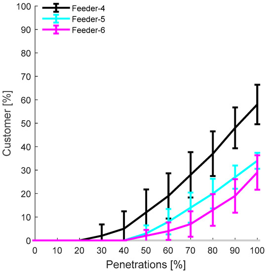
Figure 4.
Percentage of customers with voltage rise problem.
4.5. Curves Identification through Regression Analysis
Regression analysis is performed to produce models to predict the maximum voltage based on the measured power drawn by the busbar. For a given penetration level, the mean values of daily transformer active power drawn are plotted against the corresponding daily maximum voltages so as to find the equation and correlation coefficient. To capture the relationship between the maximum voltage of the network and active power injected into the network, regression analysis is, considering all daily PV penetration levels, carried out in Figure 5 (Vreg is set to 416 V as typically practiced in the UK). The correlation coefficient () is obtained as 0.78, which indicates high correlation. In line with the result obtained above, the results for minute by minute (i.e., considering resolution) should be compared in order to capture more accurate correlations (i.e., when maximum voltage occurs, power to the busbar increase). The corresponding results denote higher correlation as shown in Figure 6 at 100% PV penetration. Given the fact that power injected into the transformer has a direct relationship with the time of the voltage rise, the correlation coefficient is obtained as almost one, which indicates far more correlation (statistically perfect correlation). The result gained here can be obtained for each penetration level, and the tap position could be identified through the equation (obtained by linear regression analysis) at the corresponding penetration level. Since the voltage level changes all day long at the secondary side of the transformer, this analysis was repeated for each LV busbar voltage to be as comprehensive as possible, as shown in Figure 7. Therefore, to investigate further correlation, the penetration of PV systems and combination of all PV penetration level-based measurements can be utilized (minute by minute) to capture the real impact. To this end, it is unnecessary to use separate equations for each penetration level. The approach is inclusive, straightforward, and more viable. However, a large number of equations are obtained (i.e., considering eleven vreg settings and the corresponding eleven penetration levels lead to ninety-nine equations), and, hence, this makes the approach unviable. Consequently, the largest PV penetration level for a given vreg setting could be chosen to cover the largest reverse power. From the regression analysis, the corresponding equation coefficients (i.e., and coefficients) could be employed in control logic. It is noteworthy that in each analysis, the correlation coefficient is found to be above 0.99 (statistically, when is above 0.99, it is defined as fully correlated).
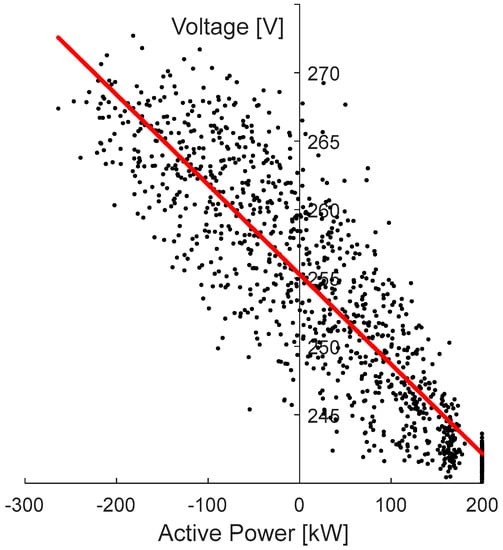
Figure 5.
Maximum voltage in the day versus the corresponding active power drawn by the transformer.
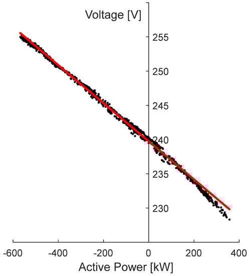
Figure 6.
Maximum voltages in each household at 100% PV penetration level (minute by minute).
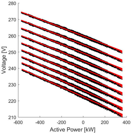
Figure 7.
Active mean power drawn by transformer versus maximum voltage on the network considering all penetration levels (minute by minute).
4.6. OLTC-Control Logic Implementation
By applying the Monte Carlo method from 0 to 100% PV penetration levels (with an increment of 10 percent) for different Vreg settings, the corresponding coefficients in each PV penetration level are captured. For each Vreg setting, , and the corresponding correlation coefficient for 100% PV penetration level are all provided in Table 1 (the reactive power coefficients are very small as expected). These values could be embedded to estimation-based local OLTC control logic so as to operate the tap changer in the most appropriate manner. Bear in mind that the tap position is expected to lower the voltage rise, yet, in the case of late triggering, a voltage rise might occur. Therefore, the voltage rise triggering set cannot be adopted high. However, when the chosen setting is too low, this will lead to higher tap operations. In this case study, the time delay for actions is 1 min.

Table 1.
Coefficients to estimate maximum voltage in the network.
In a given simulation, customer demand and PV output are chosen from the matrix for the same household and presented in Figure 8. This shows how significant voltage reduction benefits from the adoption of OLTCs for the maximum voltage in the network to be obtained. It can be observed from the figure that the tap is positioned at the maximum level, which indicates that no room is left for improvement (the best potential improvement is covered). Thus, the performance could be considered as the maximum benefit that the proposed control approach can offer.
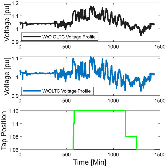
Figure 8.
Voltage profile at the last customer (at Feeder-3) and tap position (green line) at 100% PV penetration level.
In order to realistically assess the effectiveness of the decentralized control approach, the impact analysis for different control cycles is shown in Figure 9. Analysis results indicate the effectiveness of the hosting capacity for the 5 and 10 min control cycle in the first row from left to right, and the 20 and 30 min control cycle in the second row. It is evident that for different control cycles, the performance of the adopted control strategy brings benefits to the network. All feeders (except Feeder-4) manage to keep their voltage within statutory limits (BS EN50160) for the 5 min control cycle. Even Feeder-4 denotes significant improvement in terms of hosting capacity.
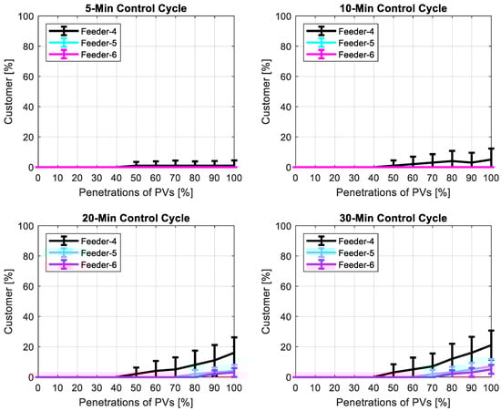
Figure 9.
Hosting capacity for different control cycles.
With larger control cycles, customers with voltage rise issues appear with different feeders. Furthermore, the number of customers having voltage rise issues increases with greater control cycles. The number of tap operations in different control cycles is shown in the box plot in Figure 10, in which it is evident that with greater control cycles, tap operations decrease. Therefore, a DNO can adopt the strategy to use a larger control cycle till technical issues emerge. Afterward, a lower control cycle will facilitate the higher hosting capacity.
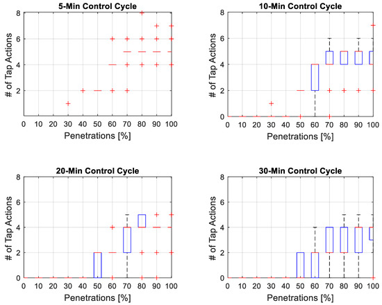
Figure 10.
The number of tap actions for different control cycles using Boxplots.
It is also found the computational complexity of the OLTC control logic is relatively low. In particular, only a few seconds are required to define the set points of the OLTC. This is due to the limited number of inputs and the simple linear mathematical models. In addition, the definition of control actions does not require registering previous power flow measurements (i.e., small memory requirements).
5. Discussions and Implementation Aspects
A real UK LV residential underground network is studied by altering the tap position in OLTC-fitted transformers in case studies; therefore, the results are subject to change for the networks of different regions/countries. Nonetheless, similar results are expected to be observed as the method is generic and can be used in any network. The corresponding settings can be straightforwardly found by DNOs. In a real-world application, the number of residents in a household and the size of the PV panel are known, therefore randomizing all these parameters may not represent the reality. These values can be added to the corresponding matrices in such a way that greater PV penetration levels cover that of lower ones. The curves resulting from regression analysis can be found in an easy manner to apply the method to any network. In order to avoid unnecessary tap operation, DNOs could take action when voltage rise occurs (30% PV penetration level in this case). Furthermore, the proposed control logic could be adopted using larger control cycles greater than a particular PV penetration level (i.e., 50% PV penetration level in this case).
For a penetration level larger than 50%, a lower control cycle could be used to boost the hosting capacity of the network (e.g., control cycle of 5 min). As the tap position is located at its maximum level, the negative impact could lead to another issue (voltage drop). Therefore, control logic considers that voltage drops (DNOs) should be put in place (considering only demand) to avoid further voltage drops for the particularly demanding drive hours. Given the OLTC is likely to boost the hosting capacity of a network along with the number of the customers with voltage problems even at the maximum PV penetration level, it could also facilitate the performance of other potential solutions. The OLTC can be controlled via remotely using measurement devices at the expense of extensive communication infrastructure/costs. However, it is more challenging to coordinate it with other potential solutions adopted in LV networks.
Further, it is worth highlighting that it might be important in practice to define seasonal-based mathematical models to provide better voltage management, particularly with the integration of other low-carbon technologies such as Electrical Vehicles (EVs). In addition, the performance of the approach could be improved by considering weather-dependent parameters (e.g., ambient temperature and irradiance) and the day of the week (e.g., weekday, weekend) in the definition of the mathematical models. Another important aspect that has to be explored to implement the proposed approach in practice is to better understand the effects of sudden variations in the supply voltage (e.g., due to interruptions) and the existence of harmonics in LV networks.
6. Conclusions
This work presents a decentralized control approach to operate an On-Load Tap Changer (OLTC) using local measurements at a distribution transformer to mitigate the impacts of Photovoltaics (PV) on Low Voltage (LV) networks. Taking into account the limited available local measurements, the control approach is driven by models that are defined offline to estimate the maximum and the minimum voltages in the network. The estimation of voltages is carried out for each control cycle using both the power flows throughout the distribution transformer and the voltage at the secondary side of the transformer. The models to estimate voltages are extracted offline by the application of the curve-fitting technique to a dataset of power flows at the distribution transformer and customers’ voltages for different PV penetrations. The dataset is produced by utilizing Monte Carlo simulations to cater for uncertainties in demand and PV generation. The approach is applied to a real UK LV feeder. Further, key performance metrics are considered, in particular, the PV hosting capacity and the number of tap actions.
The results demonstrate the linear correlation between the active power from the LV busbar and the maximum voltage rise. Further, the control approach enables significant hosting capacity improvement along with the small number of tap operations. This shows that it is possible to manage LV network voltages using local control approaches without the need to obtain remote measurements; therefore, no communication infrastructure is needed. In particular, the estimation of maximum and minimum voltages is found to be responsive to voltage changes in real time. Thus, the proposed OLTC control logic can provide guidance to DNOs in order to implement OLTC in their real networks.
Author Contributions
Conceptualization, M.S.A., S.W.A. and S.Z.A.; methodology, M.S.A., S.W.A. and S.Z.A.; software, M.S.A.; supervision, S.W.A.; writing—original draft, M.S.A.; writing—review & editing, S.W.A. and S.Z.A. All authors have read and agreed to the published version of the manuscript.
Funding
This research received no external funding.
Institutional Review Board Statement
Not applicable.
Informed Consent Statement
Not applicable.
Data Availability Statement
Not applicable.
Conflicts of Interest
The authors declare no conflict of interest.
References
- Enabling High Penetration of Solar PV in Electricity Grids; IEA: Paris, France, 2021.
- Irena, I. Renewable Energy Policies in a Time of Transition. IRENA OECD/IEA and REN21. 2018. Available online: https://www.irena.org/-/media/Files/IRENA/Agency/Publication/2018/Apr/IRENA_IEA_REN21_Policies_2018.pdf (accessed on 27 May 2022).
- Mulenga, E.; Bollen, M.H.; Etherden, N. A review of hosting capacity quantification methods for photovoltaics in low-voltage distribution grids. Int. J. Electr. Power Energy Syst. 2020, 115, 105445. [Google Scholar] [CrossRef]
- Alnaser, S.; Ochoa, L.N. Final Report for WP 1.1 and 1.2 Wide-Scale Adoption of PV in UK Distribution Networks. 2017. Available online: https://www.researchgate.net/publication/313038816_Final_Report_for_WP_11_and_12_Wide-Scale_Adoption_of_PV_in_UK_Distribution_Networks (accessed on 27 May 2022).
- Ding, F.; Mather, B. On distributed PV hosting capacity estimation, sensitivity study, and improvement. IEEE Trans. Sustain. Energy 2016, 8, 1010–1020. [Google Scholar] [CrossRef]
- Ghosh, S.; Rahman, S.; Pipattanasomporn, M. Distribution voltage regulation through active power curtailment with PV inverters and solar generation forecasts. IEEE Trans. Sustain. Energy 2016, 8, 13–22. [Google Scholar] [CrossRef]
- Riesen, Y.; Ballif, C.; Wyrsch, N. Control algorithm for a residential photovoltaic system with storage. Appl. Energy 2017, 202, 78–87. [Google Scholar] [CrossRef] [Green Version]
- Salpakari, J.; Lund, P. Optimal and rule-based control strategies for energy flexibility in buildings with PV. Appl. Energy 2016, 161, 425–436. [Google Scholar] [CrossRef] [Green Version]
- Latif, A.; Gawlik, W.; Palensky, P. Quantification and mitigation of unfairness in active power curtailment of rooftop photovoltaic systems using sensitivity based coordinated control. Energies 2016, 9, 436. [Google Scholar] [CrossRef] [Green Version]
- Alnaser, S.W.; Althaher, S.Z.; Long, C.; Zhou, Y.; Wu, J.; Hamdan, R. Transition towards solar Photovoltaic Self-Consumption policies with Batteries: From the perspective of distribution networks. Appl. Energy 2021, 304, 117859. [Google Scholar] [CrossRef]
- de Din, E.; Bigalke, F.; Pau, M.; Ponci, F.; Monti, A. Analysis of a multi-timescale framework for the voltage control of active distribution grids. Energies 2021, 14, 1965. [Google Scholar] [CrossRef]
- Zarco-Soto, F.; Zarco-Periñán, J.; Martínez-Ramos, J.L. Centralized Control of Distribution Networks with High Penetration of Renewable Energies. Energies 2021, 14, 4283. [Google Scholar] [CrossRef]
- Hashemi, S.; Østergaard, J. Methods and strategies for overvoltage prevention in low voltage distribution systems with PV. IET Renew. Power Gener. 2017, 11, 205–214. [Google Scholar] [CrossRef] [Green Version]
- Rauma, K.; Cadoux, F.; Hadj-SaïD, N.; Dufournet, A.; Baudot, C.; Roupioz, G. Assessment of the MV/LV on-load tap changer technology as a way to increase LV hosting capacity for photovoltaic power generators. In Proceedings of the CIRED Workshop 2016, Helsinki, Finland, 14–15 June 2016. [Google Scholar] [CrossRef] [Green Version]
- Paoli, J.; Brinkmann, B.; Negnevitsky, M. A practical approach to optimising distribution transformer tap settings. Energies 2020, 13, 4889. [Google Scholar] [CrossRef]
- Körner, C.; Hennig, M.; Schmid, R.; Handt, K. Gaining experience with a regulated distribution transformer in a smart grid environment. In Proceedings of the CIRED 2012 Workshop, Lisbon, Portugal, 29–30 May 2012. [Google Scholar]
- Ground Mounted Distribution Transformers; Electricity North West Limited: Warrington, UK, 2020.
- Chicco, G.C.; Spertino, F. Benefits of On-Load Tap Changers Coordinated Operation for Voltage Control in Low Voltage Grids with High Photovoltaic Penetration. In Proceedings of the 2020 International Conference on Smart Energy Systems and Technologies (SEST), Istanbul, Turkey, 13–14 September 2020; pp. 1–6. [Google Scholar]
- Ku, T.-T.; Lin, C.-H.; Chen, C.-S.; Hsu, C.-T. Coordination of transformer on-load tap changer and PV smart inverters for voltage control of distribution feeders. IEEE Trans. Ind. Appl. 2018, 55, 256–264. [Google Scholar] [CrossRef]
- Ku, T.-T.; Lin, C.-H.; Chen, C.-S.; Hsu, C.-T. An OLTC-inverter coordinated voltage regulation method for distribution network with high penetration of PV generations. Int. J. Electr. Power Energy Syst. 2019, 113, 991–1001. [Google Scholar]
- Li, C.; Disfani, V.R.; Pecenak, Z.K.; Mohajeryami, S.; Kleissl, J. Optimal OLTC voltage control scheme to enable high solar penetrations. Electr. Power Syst. Res. 2018, 160, 318–326. [Google Scholar] [CrossRef] [Green Version]
- Shukla, S.R.; Paudyal, S.; Almassalkhi, M.R. Efficient Distribution System Optimal Power Flow with Discrete Control of Load Tap Changers. IEEE Trans. Power Syst. 2019, 34, 2970–2979. [Google Scholar] [CrossRef]
- Long, C.; Ochoa, L.F. Voltage control of PV-rich LV networks: OLTC-fitted transformer and capacitor banks. IEEE Trans. Power Syst. 2015, 31, 4016–4025. [Google Scholar] [CrossRef]
- Rauma, K.; Cadoux, F.; Roupioz, G.; Dufournet, A.; Hadj-Said, N. Optimal location of voltage sensors in low voltage networks for on-load tap changer application. IET Gener. Transm. Distrib. 2017, 11, 3756–3764. [Google Scholar] [CrossRef]
- Karagiannopoulos, S.; Aristidou, P.; Hug, G. Data-driven local control design for active distribution grids using off-line optimal power flow and machine learning techniques. IEEE Trans. Smart Grid 2019, 10, 6461–6471. [Google Scholar] [CrossRef] [Green Version]
- Shahid, S.; Shafiq, S.; Khan, B.; Al-Awami, A.T.; Butt, M.O. A Machine Learning-Based Communication-Free PV Controller for Voltage Regulation. Sustainability 2021, 13, 12208. [Google Scholar] [CrossRef]
- Rylander, M.; Smith, J. Stochastic Analysis to Determine Feeder Hosting Capacity for Distributed Solar PV; Technical Report; Electric Power Research Institute: Palo Alto, CA, USA, 2012. [Google Scholar]
- Mai, T.T.; Salazar, M.; Haque, N.A.; Nguyen, P.H. Stochastic modelling of the correlation between transformer loading and distributed energy resources in LV distribution networks. In Proceedings of the CIRED 2020 Berlin Workshop, Berlin, Germany, 22–23 September 2020; pp. 480–483. [Google Scholar]
- Richardson, I.; Thomson, M.; Infield, D.; Clifford, C. Domestic electricity use: A high-resolution energy demand model. Energy Build. 2010, 42, 1878–1887. [Google Scholar] [CrossRef] [Green Version]
- Alnaser, S.W.; Althaher, S.Z.; Long, C.; Zhou, Y.; Wu, J. Residential community with PV and batteries: Reserve provision under grid constraints. Int. J. Electr. Power Energy Syst. 2020, 119, 105856. [Google Scholar] [CrossRef]
- Low Voltage Network Models and Low Carbon Technology Profiles. Available online: https://www.enwl.co.uk/go-net-zero/innovation/smaller-projects/low-carbon-networks-fund/low-voltage-network-solutions/ (accessed on 27 May 2022).
- Dugan, R.S.; Sunderman, W. Distribution modeling and analysis of high penetration PV. In Proceedings of the 2011 IEEE Power and Energy Society General Meeting, Detroit, MI, USA, 24–27 July 2011; pp. 1–7. [Google Scholar]
- Available online: https://www.gov.uk/government/statistics/solar-photovoltaics-deployment (accessed on 27 May 2022).
- The Electricity Safety, Quality and Continuity Regulations; UK Department of Trade and Industry: London, UK, 2002.
Publisher’s Note: MDPI stays neutral with regard to jurisdictional claims in published maps and institutional affiliations. |
© 2022 by the authors. Licensee MDPI, Basel, Switzerland. This article is an open access article distributed under the terms and conditions of the Creative Commons Attribution (CC BY) license (https://creativecommons.org/licenses/by/4.0/).