
Relative Prices of Ethanol-Gasoline in the Major Brazilian Capitals: An Analysis to Support Public Policies


Abstract
1. Introduction
1.1. Contextualization
1.2. Objectives
1.3. Hypothesis
1.4. Justification and Contribution
2. Literature Review
3. Regional Aspects and Pricing of Ethanol and Gasoline in Brazilian Retail Market
3.1. Pricing of Gasoline and Ethanol at Retail Markets
3.2. Regional Aspects of Ethanol Supply in Brazil
4. Methods and Data
4.1. Methods
- First, 0 < H < 0.5 anti-persistent series, or simply means reversal behavior. That is, there is a greater than 50% probability that a negative value will be preceded by a positive one. The strength of this behavior will depend on how close the H is to zero;
- Second, H = 0.5 series has a random walk distribution (white noise, efficient market), meaning that it has no long memory. Thus, the variation in the cumulative deviations must increase proportionally to the square root of the time variable;
- Third, 0.5 < H < 1 persistent series, meaning there is a probability of repetition of a value above 50%;
- Fourth, H = 1 identifies a pink noise and H > 1 means that long-range dependence is not explained by a power law, but these two results are uncommon in economic and financial time series.
4.2. Data
5. Results
5.1. Analysis of the Degree of Persistence (DFA) of Ethanol/Gasoline Relative Price Returns
5.1.1. North
5.1.2. Northeast
5.1.3. Midwest
5.1.4. Southeast
5.1.5. South
5.2. Analysis of Detrended Cross-Correlations Analysis (DCCA)
5.2.1. North
5.2.2. Northeast
5.2.3. Midwest
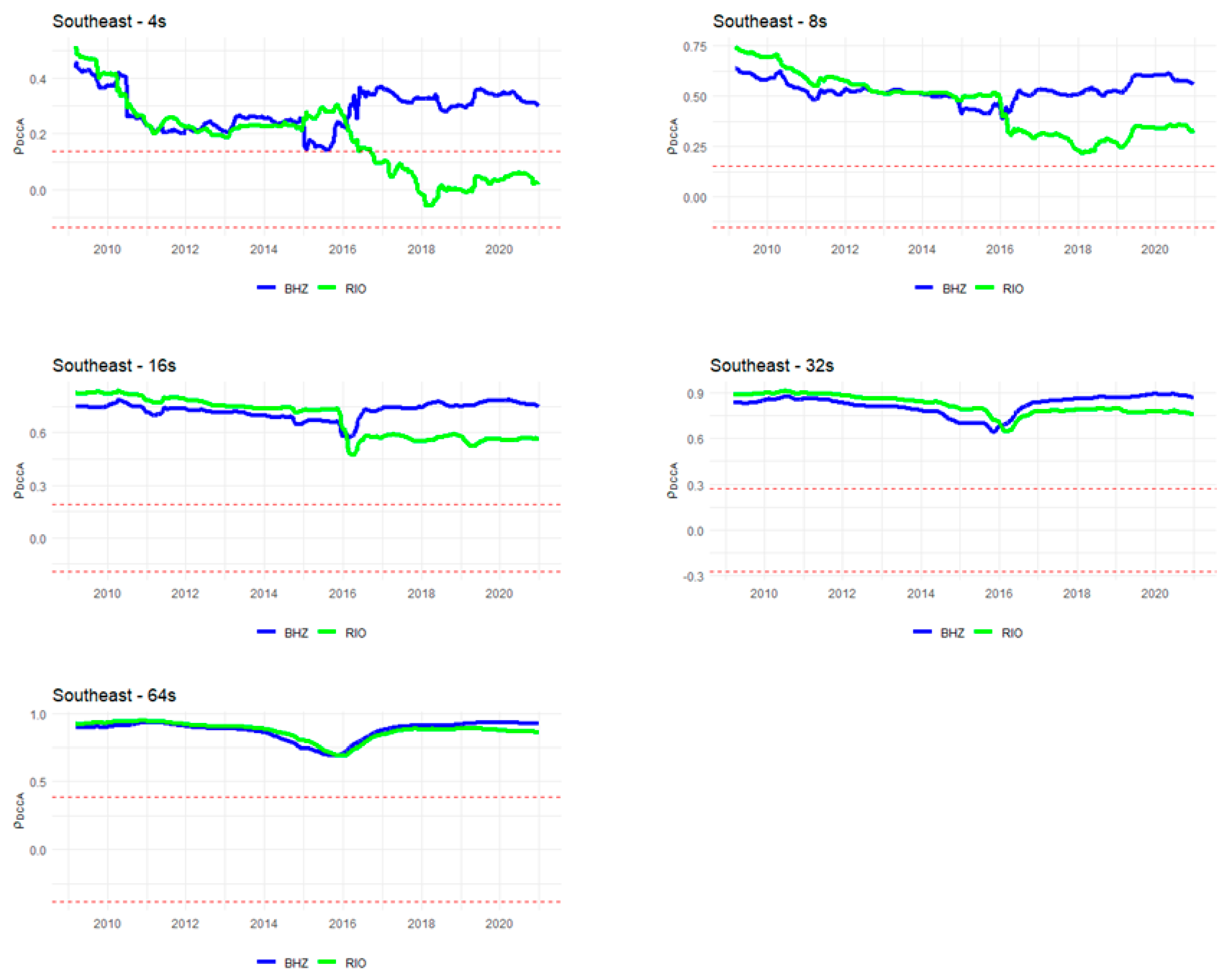
5.2.4. Southeast
5.2.5. South
5.3. Discussion of Results
6. Conclusions
6.1. Main Conclusions
6.2. Policy Implications for Private Agents and the Public Sector
6.3. Limitations and Research Agenda
Author Contributions
Funding
Institutional Review Board Statement
Informed Consent Statement
Data Availability Statement
Acknowledgments
Conflicts of Interest
References
- SINDIPEÇAS. Relatório da Frota Circulante. 2019. Available online: https://www.sindipecas.org.br/sindinews/Economia/2019/RelatorioFrotaCirculante_Maio_2019.pdf (accessed on 5 January 2022).
- Costa, C.C.D.; Burnquist, H.L. Impactos do controle do preço da gasolina sobre o etanol biocombustível no Brasil. Estud. Econômicos 2016, 46, 1003–1028. [Google Scholar] [CrossRef][Green Version]
- Figueira, S.R.; Burnquist, H.L.; Bacchi, M.R.P. Forecasting fuel ethanol consumption in Brazil by time series models: 2006–2012. Appl. Econ. 2010, 42, 865–874. [Google Scholar] [CrossRef]
- El Montasser, G.; Gupta, R.; Martins, A.L.; Wanke, P. Are there multiple bubbles in the ethanol–gasoline price ratio of Brazil? Renew. Sustain. Energy Rev. 2015, 52, 19–23. [Google Scholar] [CrossRef]
- Laurini, M.P. The spatio-temporal dynamics of ethanol/gasoline price ratio in Brazil. Renew. Sustain. Energy Rev. 2017, 70, 1–12. [Google Scholar] [CrossRef]
- Debnath, D.; Whistance, J.; Thompson, W.; Binfield, J. Complement or substitute: Ethanol’s uncertain relationship with gasoline under alternative petroleum price and policy scenarios. Appl. Energy 2017, 191, 385–397. [Google Scholar] [CrossRef]
- Fama, E.F. Efficient capital markets: II. J. Financ. 1991, 46, 1575–1617. [Google Scholar] [CrossRef]
- Barros, C.P.; Gil-Alana, L.A.; Wanke, P. Ethanol consumption in Brazil: Empirical facts based on persistence, seasonality and breaks. Biomass Bioenergy 2014, 63, 313–320. [Google Scholar] [CrossRef]
- Nascimento Filho, A.S.; Saba, H.; dos Santos, R.G.; Calmon, J.G.A.; Araújo, M.L.; Jorge, E.M.; Murari, T.B. Analysis of Hydrous Ethanol Price Competitiveness after the Implementation of the Fossil Fuel Import Price Parity Policy in Brazil. Sustainability 2021, 13, 9899. [Google Scholar] [CrossRef]
- Samanez, C.P.; da Rocha Ferreira, L.; do Nascimento, C.C.; de Almeida Costa, L.; Bisso, C.R. Evaluating the economy embedded in the Brazilian ethanol-gasoline flex-fuel car: A real options approach. Appl. Econ. 2014, 46, 1565–1581. [Google Scholar] [CrossRef]
- David, S.A.; Inacio Junior, C.M.C.; Quintino, D.D.; Machado, J.A.T. Measuring the Brazilian ethanol and gasoline market efficiency using DFA-Hurst and fractal dimension. Energy Econ. 2020, 85, 104614. [Google Scholar] [CrossRef]
- Da Costa, C.C.; Burnquist, H.L.; Guilhoto, J.J.M. The Impact of Changes in Fuel Policies on the Brazilian Economy. Econ. Apl. 2017, 21, 635–657. [Google Scholar]
- Janda, K.; Kristoufek, L. The relationship between fuel and food prices: Methods and outcomes. Annu. Rev. Resour. Econ. 2019, 11, 195–216. [Google Scholar] [CrossRef]
- Quintino, D.D.; David, S.A.; Vian, C.E.F. Analysis of the relationship between ethanol spot and futures prices in Brazil. Int. J. Financ. Stud. 2017, 5, 11. [Google Scholar] [CrossRef]
- Capitani, D.H.D.; Junior, J.C.C.; Tonin, J.M. Integration and hedging efficiency between Brazilian and US ethanol markets. Contextus–Rev. Contemp. De Econ. E Gestão 2018, 16, 93–117. [Google Scholar]
- Dutta, A. Are global ethanol markets a ‘one great pool’? Biomass Bioenergy 2020, 132, 105–436. [Google Scholar] [CrossRef]
- Hernandez, J.A.; Uddin, G.S.; Dutta, A.; Ahmed, A.; Kang, S.H. Are ethanol markets globalized or regionalized? Phys. A Stat. Mech. Appl. 2020, 551, 124094. [Google Scholar] [CrossRef]
- Quintino, D.D.; Cantarinha, A.; Ferreira, P.J.S. Relationship between US and Brazilian ethanol prices: New evidence based on fractal regressions. Biofuels Bioprod. Biorefining 2021, 15, 1215–1220. [Google Scholar] [CrossRef]
- Palazzi, R.B.; Meira, E.; Klotzle, M.C. The sugar-ethanol-oil nexus in Brazil: Exploring the pass-through of international commodity prices to national fuel prices. J. Commod. Mark. 2022, 100257. [Google Scholar] [CrossRef]
- Dutta, A.; Bouri, E. Carbon emission and ethanol markets: Evidence from Brazil. Biofuels Bioprod. Biorefining 2019, 13, 458–463. [Google Scholar] [CrossRef]
- Uddin, G.S.; Hernandez, J.A.; Wadström, C.; Dutta, A.; Ahmed, A. Do uncertainties affect biofuel prices? Biomass Bioenergy 2021, 148, 106006. [Google Scholar] [CrossRef]
- David, S.A.; Quintino, D.D.; Inacio Junior, C.M.C.; Machado, J.T. Fractional dynamic behavior in ethanol prices series. J. Comput. Appl. Math. 2018, 339, 85–93. [Google Scholar] [CrossRef]
- Almeida, E.L.F.D.; Oliveira, P.V.D.; Losekann, L. Impactos da contenção dos preços de combustíveis no Brasil e opções de mecanismos de precificação. Rev. Bras. De Econ. Política 2015, 35, 531–556. [Google Scholar] [CrossRef]
- Quintino, D.D.; David, S.A. Quantitative analysis of feasibility of hydrous ethanol futures contracts in Brazil. Energy Econ. 2013, 40, 927–935. [Google Scholar] [CrossRef]
- Marjotta-Maistro, M.C.; Barros, G.S.A.D.C. Relações comerciais e de preços no mercado nacional de combustíveis. Rev. De Econ. E Sociol. Rural. 2003, 41, 829–858. [Google Scholar] [CrossRef][Green Version]
- Moraes, M.A.F.D.; Zilberman, D. Production of Ethanol from Sugarcane in Brazil: From State Intervention to a Free Market; Springer Science & Business Media: Berlin/Heidelberg, Germany, 2014; Volume 43. [Google Scholar]
- Paulillo, L.F.; Soares, S.S.; Feltre, C.; Marques, D.S.P.; Vian, C.E.F. As transformações e os desafios do encadeamento produtivo do etanol no Brasil. In Quarenta Anos de Etanol em Larga Escala no Brasil; IPEA: Brasília, Brazil, 2016; p. 187. Available online: https://www3.eco.unicamp.br/nea/images/arquivos/Book_Quarenta_Anos_de_Etanol.pdf (accessed on 17 January 2022).
- EPE. Empresa de Pesquisa Energética. Série de Formação de Preços de Combustíveis: Margem Bruta de Distribuição e Revenda. 2020. Available online: https://www.epe.gov.br/sites-pt/publicacoes-dados-abertos/publicacoes/PublicacoesArquivos/publicacao-413/topico-476/SP-EPE-DPG-SDB-Abast-02-2019_DistrRev.pdf (accessed on 25 February 2021).
- ANP. Anuário Estatístico Brasileiro de Petróleo, Gás Natural e Biocombustíveis 2020. 2020. Available online: https://www.gov.br/anp/pt-br/centrais-de-conteudo/publicacoes/anuario-estatistico/arquivos-anuario-estatistico-2020/anuario-2020.pdf (accessed on 1 June 2021).
- Da Silva, A.S.; Vasconcelos, C.R.F.; Vasconcelos, S.P.; de Mattos, R.S. Symmetric transmission of prices in the retail gasoline market in Brazil. Energy Econ. 2014, 43, 11–21. [Google Scholar] [CrossRef]
- Margarido, M.A.; Dos Santos, G.R.; Vian, C.E.F.; Shikida, P.A.; Bauermann, B.C. CIDE and elasticity oscillation on the ethanol and gasoline market: Brazilian taxation policy under discussion. Ital. Rev. Agric. Econ. 2020, 75, 3–17. [Google Scholar]
- EPE. Empresa de Pesquisa Energética. Série de Formação de Preços de Combustíveis: Tributos Incidentes Sobre a Comercialização de Combustíveis no Brasil. 2020. Available online: https://www.epe.gov.br/sites-pt/publicacoes-dados-abertos/publicacoes/PublicacoesArquivos/publicacao-413/topico-562/SP-EPE-DPG-SDB-Abast-01-2020_Tributos_comercializa%C3%A7%C3%A3o.pdf (accessed on 25 February 2021).
- Mączyńska, J.; Krzywonos, M.; Kupczyk, A.; Tucki, K.; Sikora, M.; Pińkowska, H.; Wielewska, I. Production and use of biofuels for transport in Poland and Brazil–The case of bioethanol. Fuel 2019, 241, 989–996. [Google Scholar] [CrossRef]
- Vian, C.E.F. Agroindústria Canavieira: Estratégias Competitivas e Modernização; Editora Átomo: Rio de Janeiro, Brazil, 2003. [Google Scholar]
- Moraes, M.L.D.; Bacchi, M.R.P. Etanol: Do início às fases atuais de produção. Rev. De Política Agrícola 2015, 23, 5–22. [Google Scholar]
- Zilio, L.B.; Lima, R.A.D.S. Atratividade de canaviais paulistas sob a ótica da Teoria das Opções Reais. Rev. De Econ. E Sociol. Rural 2015, 53, 377–394. [Google Scholar] [CrossRef]
- Granco, G.; Caldas, M.M.; Bergtold, J.S.; Sant’Anna, A.C. Exploring the policy and social factors fueling the expansion and shift of sugarcane production in the Brazilian Cerrado. GeoJournal 2017, 82, 63–80. [Google Scholar] [CrossRef]
- ANP. Anuário Estatístico Brasileiro de Petróleo, Gás Natural e Biocombustíveis 2010. 2010. Available online: https://www.gov.br/anp/pt-br/centrais-de-conteudo/publicacoes/anuario-estatistico/arquivos-anuario-estatistico-2010/versao-para-impressao.pdf (accessed on 1 June 2021).
- Peng, C.K.; Buldyrev, S.V.; Havlin, S.; Simons, M.; Stanley, H.E.; Goldberger, A.L. On the mosaic organization of DNA sequences. Phys. Rev. E 1994, 49, 1685–1689. [Google Scholar] [CrossRef] [PubMed]
- Hwa, R.C.; Ferree, T.C. Scaling properties of fluctuations in the human electroencephalogram. Phys. Rev. E 2002, 66, 021901. [Google Scholar] [CrossRef] [PubMed]
- Mohti, W.; Dionísio, A.; Ferreira, P.; Vieira, I. Frontier markets’ efficiency: Mutual information and detrended fluctuation analyses. J. Econ. Interact. Coord. 2019, 14, 551–572. [Google Scholar] [CrossRef]
- Chen, Z.; Ivanov, P.C.; Hu, K.; Stanley, H.E. Effect of nonstationarities on detrended fluctuation analysis. Phys. Rev. E 2002, 65, 041107. [Google Scholar] [CrossRef]
- Hu, K.; Ivanov, P.C.; Chen, Z.; Carpena, P.; Stanley, H.E. Effect of trends on detrended fluctuation analysis. Phys. Rev. E 2001, 64, 011114. [Google Scholar] [CrossRef]
- Kantelhardt, J.W.; Zschiegner, S.A.; Koscielny-Bunde, E.; Havlin, S.; Bunde, A.; Stanley, H.E. Multifractal detrended fluctuation analysis of nonstationary time series. Phys. A Stat. Mech. Appl. 2002, 316, 87–114. [Google Scholar] [CrossRef]
- Cajueiro, D.O.; Tabak, B.M. The Hurst exponent over time: Testing the assertion that emerging markets are becoming more efficient. Phys. A Stat. Mech. Appl. 2004, 336, 521–537. [Google Scholar] [CrossRef]
- Cajueiro, D.O.; Tabak, B.M. Evidence of long range dependence in Asian equity markets: The role of liquidity and market restrictions. Phys. A Stat. Mech. Appl. 2004, 342, 656–664. [Google Scholar] [CrossRef]
- Alvarez-Ramirez, J.; Rodriguez, E.; Ibarra-Valdez, C. Long-range correlations and asymmetry in the Bitcoin market. Phys. A Stat. Mech. Appl. 2018, 492, 948–955. [Google Scholar] [CrossRef]
- Ferreira, P. Dynamic long-range dependences in the Swiss stock market. Empir. Econ. 2020, 58, 1541–1573. [Google Scholar] [CrossRef]
- Zebende, G.F. DCCA cross-correlation coefficient: Quantifying level of cross-correlation. Phys. A Stat. Mech. Appl. 2011, 390, 614–618. [Google Scholar] [CrossRef]
- Podobnik, B.; Stanley, H.E. Detrended cross-correlation analysis: A new method for analyzing two nonstationary time series. Phys. Rev. Lett. 2008, 100, 084102. [Google Scholar] [CrossRef] [PubMed]
- Kristoufek, L. Measuring correlations between non-stationary series with DCCA coefficient. Phys. A Stat. Mech. Appl. 2014, 402, 291–298. [Google Scholar] [CrossRef]
- Kristoufek, L. Detrending moving-average cross-correlation coefficient: Measuring cross-correlations between non-stationary series. Phys. A Stat. Mech. Appl. 2014, 406, 169–175. [Google Scholar] [CrossRef]
- Wang, G.J.; Xie, C.; Chen, Y.J.; Chen, S. Statistical properties of the foreign exchange network at different time scales: Evidence from detrended cross-correlation coefficient and minimum spanning tree. Entropy 2013, 15, 1643–1662. [Google Scholar] [CrossRef]
- Zhao, X.; Shang, P.; Huang, J. Several fundamental properties of DCCA cross-correlation coefficient. Fractals 2017, 25, 1750017. [Google Scholar] [CrossRef]
- Reboredo, J.C.; Rivera-Castro, M.A.; Zebende, G.F. Oil and US dollar exchange rate dependence: A detrended cross-correlation approach. Energy Econ. 2014, 42, 132–139. [Google Scholar] [CrossRef]
- Pal, D.; Mitra, S.K. Interdependence between crude oil and world food prices: A detrended cross correlation analysis. Phys. A Stat. Mech. Appl. 2018, 492, 1032–1044. [Google Scholar] [CrossRef]
- Paiva, A.S.S.; Rivera-Castro, M.A.; Andrade, R.F.S. DCCA analysis of renewable and conventional energy prices. Phys. A Stat. Mech. Appl. 2018, 490, 1408–1414. [Google Scholar] [CrossRef]
- Nascimento Filho, A.S.; Pereira, E.J.A.L.; Ferreira, P.; Murari, T.B.; Moret, M.A. Cross-correlation analysis on Brazilian gasoline retail market. Phys. A Stat. Mech. Appl. 2018, 508, 550–557. [Google Scholar] [CrossRef]
- Mitra, S.K.; Bhatia, V.; Jana, R.K.; Charan, P.; Chattopadhyay, M. Changing value detrended cross correlation coefficient over time: Between crude oil and crop prices. Phys. A Stat. Mech. Appl. 2018, 506, 671–678. [Google Scholar] [CrossRef]
- Murari, T.B.; Nascimento Filho, A.S.; Pereira, E.J.; Ferreira, P.; Pitombo, S.; Pereira, H.B.; Moret, M.A. Comparative analysis between hydrous ethanol and gasoline c pricing in Brazilian retail market. Sustainability 2019, 11, 4719. [Google Scholar] [CrossRef]
- Lima, C.R.A.; de Melo, G.R.; Stosic, B.; Stosic, T. Cross-correlations between Brazilian biofuel and food market: Ethanol versus sugar. Phys. A Stat. Mech. Appl. 2019, 513, 687–693. [Google Scholar] [CrossRef]
- Fan, X.; Li, X.; Yin, J. Dynamic relationship between carbon price and coal price: Perspective based on Detrended Cross-Correlation Analysis. Energy Procedia 2019, 158, 3470–3475. [Google Scholar] [CrossRef]
- Ferreira, P.; Loures, L.C. An Econophysics Study of the S&P Global Clean Energy Index. Sustainability 2020, 12, 662. [Google Scholar]
- Casa Nova, A.; Ferreira, P.; Almeida, D.; Dionísio, A.; Quintino, D. Are Mobility and COVID-19 Related? A Dynamic Analysis for Portuguese Districts. Entropy 2021, 23, 786. [Google Scholar] [CrossRef]
- ANP. Série Histórica do Levantamento de Preços. 2021. Available online: https://www.gov.br/anp/pt-br/assuntos/precos-e-defesa-da-concorrencia/precos/precos-revenda-e-de-distribuicao-combustiveis/serie-historica-do-levantamento-de-precos (accessed on 1 June 2021).
- Podobnik, B.; Jiang, Z.Q.; Zhou, W.X.; Stanley, H.E. Statistical tests for power-law cross-correlated processes. Phys. Rev. E 2011, 84, 066118. [Google Scholar] [CrossRef]
- Ferreira, P. Long-range dependencies of Eastern European stock markets: A dynamic detrended analysis. Phys. A Stat. Mech. Appl. 2018, 505, 454–470. [Google Scholar] [CrossRef]
- Tilfani, O.; Ferreira, P.; El Boukfaoui, M.Y. Dynamic cross-correlation and dynamic contagion of stock markets: A sliding windows approach with the DCCA correlation coefficient. Empir. Econ. 2019, 60, 1127–1156. [Google Scholar] [CrossRef]
- Guedes, E.F.; Zebende, G.F. DCCA cross-correlation coefficient with sliding windows approach. Phys. A Stat. Mech. Appl. 2019, 527, 121286. [Google Scholar] [CrossRef]
- PETROBRÁS. Refinarias. 2022. Available online: https://petrobras.com.br/pt/nossas-atividades/principais-operacoes/refinarias/ (accessed on 13 January 2022).
- ESTADÃO. Cade vai Monitorar o Preço dos Combustíveis em Postos de todo o País. 2021. Available online: https://economia.estadao.com.br/noticias/geral,cade-vai-monitorar-o-preco-de-combustiveis-em-postos-de-todo-o-pais,70003621206 (accessed on 25 February 2021).


| Distributor | Gasoline C | Hydrous Ethanol |
|---|---|---|
| BR | 23.40% | 16.70% |
| Ipiranga | 19.30% | 17.10% |
| Raízen | 16.90% | 19.40% |
| Others | 40.40% | 46.80% |
| Period | Brazil | N | % (N) | NE | % (NE) | SE | % (SE) | S | % (S) | M | % (M) | Total |
|---|---|---|---|---|---|---|---|---|---|---|---|---|
| 2001–2005 (P1) | 6158.5 | 11.6 | 0.2% | 755.5 | 12.3% | 3851.7 | 62.5% | 661.3 | 10.7% | 878.4 | 14.3% | 100.0% |
| 2006–2010 (P2) | 16,193.3 | 33.7 | 0.2% | 1035.7 | 6.4% | 11,063.1 | 68.3% | 1378.7 | 8.5% | 2682.1 | 16.6% | 100.0% |
| 2011–2015 (P3) | 15,772.6 | 84.6 | 0.5% | 800.5 | 5.1% | 8858.6 | 56.2% | 986.4 | 6.3% | 5042.5 | 32.0% | 100.0% |
| 2016–2020 (P4) | 21,014.1 | 94.4 | 0.4% | 962.0 | 4.6% | 11,574.4 | 55.1% | 900.5 | 4.3% | 7482.7 | 35.6% | 100.0% |
| Var % | ||||||||||||
| 2006–2010 (P2/P1) | 162.9% | 190.6% | 37.1% | 187.2% | 108.5% | 205.3% | ||||||
| 2011–2015 (P3/P2) | −2.6% | 151.0% | −22.7% | −19.9% | −28.5% | 88.0% | ||||||
| 2016–2020 (P4/P3) | 33.2% | 11.7% | 20.2% | 30.7% | −8.7% | 48.4% |
| Region | City | Latitude | Longitude |
|---|---|---|---|
| North | Belém (BEL) | −1.382051 | −48.477898 |
| Manaus (MAO) | −3.036105 | −60.046593 | |
| Rio Branco (RBR) | −9.866168 | −67.897189 | |
| Northeast | Fortaleza (FOR) | −3.777554 | −38.533172 |
| Recife (REC) | −8.061129 | −34.871665 | |
| Salvador (SSA) | −12.911014 | −38.331413 | |
| Midwest | Brasília (BSB) | −15.869923 | −47.917428 |
| Cuiabá (CGB) | −15.594821 | −56.091696 | |
| Goiânia (GYN) | −16.601095 | −49.144543 | |
| Southeast | Belo Horizonte (BHZ) | −19.846098 | −43.963296 |
| Rio de Janeiro (RIO) | −22.913002 | −43.180002 | |
| São Paulo (SAO) | −23.589592 | −46.660721 | |
| South | Curitiba (CWB) | −25.442395 | −49.240417 |
| Florianópolis (FLN) | −27.670175 | −48.545944 | |
| Porto Alegre (POA) | −29.993399 | −51.175563 |
| City-Region | Id | Mean | Std Dev | CoefVar | Max | Min | Skewness | Kurtosis |
|---|---|---|---|---|---|---|---|---|
| Belém-N | BEL | 0.0002 | 0.01 | 79.98 | 0.07 | −0.09 | −0.34 | 6.06 |
| Belo Horizonte-SE | BHZ | 0.0002 | 0.01 | 79.09 | 0.05 | −0.10 | −0.76 | 5.79 |
| Brasília-M | BSB | 0.0002 | 0.02 | 99.03 | 0.16 | −0.12 | 0.47 | 8.59 |
| Cuiabá-M | CGB | 0.0003 | 0.03 | 94.75 | 0.17 | −0.16 | 0.71 | 11.30 |
| Curitiba-S | CWB | 0.0006 | 0.02 | 34.29 | 0.11 | −0.11 | 0.46 | 6.82 |
| Florianópolis-S | FLN | 0.0004 | 0.02 | 47.78 | 0.14 | −0.08 | 0.42 | 4.58 |
| Fortaleza-NE | FOR | 0.0004 | 0.02 | 38.83 | 0.10 | −0.12 | −1.82 | 11.06 |
| Goiânia-M | GYN | 0.0003 | 0.03 | 78.73 | 0.15 | −0.18 | −0.49 | 10.72 |
| Manaus-N | MAO | 0.0002 | 0.03 | 143.21 | 0.13 | −0.22 | −2.01 | 12.04 |
| Porto Alegre-S | POA | 0.0007 | 0.02 | 27.71 | 0.09 | −0.11 | −0.56 | 6.79 |
| Recife-NE | REC | 0.0004 | 0.02 | 61.67 | 0.10 | −0.13 | −1.41 | 8.51 |
| Rio Branco-N | RBR | 0.0001 | 0.01 | 89.67 | 0.10 | −0.09 | 0.25 | 13.45 |
| Rio de Janeiro-SE | RIO | 0.0005 | 0.01 | 25.83 | 0.08 | −0.05 | 0.38 | 3.36 |
| Salvador-NE | SSA | 0.0002 | 0.02 | 69.41 | 0.11 | −0.12 | −0.42 | 9.47 |
| São Paulo-SE | SAO | 0.0007 | 0.02 | 25.13 | 0.09 | −0.09 | 0.17 | 5.19 |
| City | Hurst ± StdDev |
|---|---|
| MAO-N | 0.34 ± 0.02 |
| REC-NE | 0.42 ± 0.01 |
| FOR-NE | 0.47 ± 0.03 |
| SSA-NE | 0.47 ± 0.02 |
| FLN-S | 0.49 ± 0.02 |
| GYN-M | 0.49 ± 0.03 |
| BSB-M | 0.49 ± 0.03 |
| BEL-N | 0.52 ± 0.01 |
| RBR-N | 0.52 ± 0.02 |
| CGB-M | 0.55 ± 0.03 |
| POA-S | 0.57 ± 0.03 |
| CWB-S | 0.59 ± 0.04 |
| BHZ-SE | 0.61 ± 0.03 |
| RIO-SE | 0.64 ± 0.03 |
| SAO-SE | 0.66 ± 0.04 |
Publisher’s Note: MDPI stays neutral with regard to jurisdictional claims in published maps and institutional affiliations. |
© 2022 by the authors. Licensee MDPI, Basel, Switzerland. This article is an open access article distributed under the terms and conditions of the Creative Commons Attribution (CC BY) license (https://creativecommons.org/licenses/by/4.0/).
Share and Cite
Quintino, D.D.; Burnquist, H.L.; Ferreira, P. Relative Prices of Ethanol-Gasoline in the Major Brazilian Capitals: An Analysis to Support Public Policies. Energies 2022, 15, 4795. https://doi.org/10.3390/en15134795
Quintino DD, Burnquist HL, Ferreira P. Relative Prices of Ethanol-Gasoline in the Major Brazilian Capitals: An Analysis to Support Public Policies. Energies. 2022; 15(13):4795. https://doi.org/10.3390/en15134795
Chicago/Turabian StyleQuintino, Derick David, Heloisa Lee Burnquist, and Paulo Ferreira. 2022. "Relative Prices of Ethanol-Gasoline in the Major Brazilian Capitals: An Analysis to Support Public Policies" Energies 15, no. 13: 4795. https://doi.org/10.3390/en15134795
APA StyleQuintino, D. D., Burnquist, H. L., & Ferreira, P. (2022). Relative Prices of Ethanol-Gasoline in the Major Brazilian Capitals: An Analysis to Support Public Policies. Energies, 15(13), 4795. https://doi.org/10.3390/en15134795