Article

Selecting Surface Inclination for Maximum Solar Power

by
Ioannis-Panagiotis Raptis
1,2,*,
Anna Moustaka
3,
Panagiotis Kosmopoulos
1,* and
Stelios Kazadzis
4
1
Institute for Environmental Research and Sustainable Development, National Observatory of Athens, 15236 Athens, Greece
2
Department of Geology and Geoenvironment, National and Kapodistrian University of Athens, 15784 Athens, Greece
3
Institute for Astronomy, Astrophysics, Space Applications and Remote Sensing, National Observatory of Athens, 15236 Athens, Greece
4
Physicalisch-Meteorologisches Observatorium Davos—World Radiation Center, 7260 Davos, Switzerland
*
Authors to whom correspondence should be addressed.
Energies 2022, 15(13), 4784; https://doi.org/10.3390/en15134784
Submission received: 31 May 2022 / Revised: 23 June 2022 / Accepted: 28 June 2022 / Published: 29 June 2022

Abstract

:
Maximum efficiency of surfaces that exploit solar energy, including Photovoltaic Panels and Thermal collectors, is achieved by installing them in a certain inclination (tilt). Most common approach is to select an inclination angle equal to the location’s latitude. This is based on the astronomical calculations of the sun’s position throughout the year but ignores meteorological factors. Cloud coverage and aerosols tend to change the direct irradiance but also the radiance sky distribution, thus horizontal surfaces receive larger amounts than tilted ones in specific atmospheric conditions (e.g., cases of cloud presence). In the present study we used 15 years of data, from 25 cities in Europe and North Africa in order to estimate the optimal tilt angle and the related energy benefits based in real atmospheric conditions. Data were retrieved from Copernicus Atmospheric Monitoring Service (CAMS). Four diffuse irradiance, various models are compared, and their differences are evaluated. Equations, extracted from solar irradiance and cloud properties regressions, are suggested to estimate the optimal tilt angle in regions, where no climatological data are available. In addition, the impact of cloud coverage is parameterized using the Cloud Modification Factor (CMF) and an equation is proposed to estimate the optimal tilt angle. A realistic representation of the photovoltaic energy production and a subsequent financial analysis were additionally performed. The results are able to support the prognosis of energy outcome and should be part of energy planning and the decision making for optimum solar power exploitation into the international clean energy transitions. Finally, results are compared to a global study and differences on the optimal tilt angle at cities of Northern Europe is presented.

Graphical Abstract

1. Introduction

Energy needs of societies are steadily increasing, while an urgent need of transition from fossil fuels to renewable energy sources is ascertained in studies and reports [1,2,3] Solar energy is one of the most safe and sustainable energy sources and its use is expected to rise significantly over the next decades [4,5]. Μost widely applied approach for capturing solar energy is the installation of Photovoltaic (PV) surfaces on rooftops or in PV power plants. In order to maximize the outcome of PV systems, the surfaces usually are set at certain inclinations. The most effective approach is to install a solar tracking system, that will follow the sun during the day, but this is more expensive and also consumes energy to rotate [6]. Simpler installations are set at a constant inclination. Prognosis of the solar irradiance incident on the inclined surface is crucial for evaluating the electric output and maximizing the efficiency of the system. Basic astronomic calculations provide an estimation for the tilt angle of the installation, assuming clear sky conditions (e.g., [7]). The simulation of the sun path at a specific location, during all days of year, leads to the preferred fixed angle of β equal with φ facing the equinox, where β is the optimal angle and φ the location’s latitude [8]. In real conditions, the optimum angle is different due to atmospheric processes, caused basically by clouds and secondary by other particles such as aerosols. These facts lead to different approaches when designing PV set ups, depending on energy needs, available budget and climatological data. In case of cloud covered skies, for solar tracking PVs, the energy spent for rotating the system could overpass the captured from the panel and in this case a horizontal surface would be more beneficial. Additionally, other applications, such as solar thermal collectors [9] or greenhouses covers [10], need to select the tilt angle of surfaces aiming to receive maximum solar irradiance all year round. Azimuthal orientation is always preferably southwise at the North Hemisphere and northwise at the South Hemisphere [6].
Recent studies have been published, estimating the optimum tilt angle for maximum solar energy yield, at specific geographical regions [8,11,12,13,14,15,16,17,18,19]. In addition, the question of a global tool to calculate the ideal installation setup had been studied with the use of neural networks [20], other meteorological variables [21], Genetic Algorithms [22] and Particle-Swarm Optimization techniques [23]. Jacobson and Jadhav [24] have utilized PVWatts [25] database and Chinchilla [26], two databases (EnergyPlus and Baseline Surface Raiation Network—BSRN) in order to propose a global approach on calculating the optimum tilt angle, which in each case provided better results at different geographical areas. All the above-mentioned studies conclude optimal tilt angles, smaller than the latitude but the exact values for same regions differ mainly due to different training periods/data sets and assumptions made.
The main aspect of the present work is to assess the possibility of simple and uniform equations to calculate the most effective tilt angle at a location, considering cloud climatology at the given area. This prognosis is based on the past climatology, but it will be very close to the actual conditions for the coming decades, if there are no large deviations on cloud coverage. Additionally, an approach that uses the latitude as a proxy for these parameters (which is only valid in the studied area) have been developed. In order to achieve these semiempirical approaches, we have used hourly irradiance data for 25 cities for a 15-year period by CAMS as input to a diffuse irradiance model in order to calculate the incident irradiance at different tilt angles. This historic database then is exploited in order to estimate the optimal tilt angle at each city and aggregate the results in respect to latitude and clouds. Finally, a financial analysis of the benefits is presented. Our aim is to keep the suggested approaches as simple as possible, in order to be conveniently applied by users and to give prominence of exploiting publicly available databases such as CAMS for similar applications.

2. Data and Methods

2.1. Data Sets

Hourly data for the years 2005–2019 for 25 cities in Europe and North Africa (as shown in Figure 1), were used. This service can provide global (GHI), beam (BHI), diffuse (DHI) irradiance on horizontal plane at ground level for cloudless and real sky conditions and the irradiation on horizontal plane at the top of the atmosphere. These datasets are created by combining satellite images and model calculations for cloudless conditions, following the Heliosat-4 method [27].
Τhe following quality control criteria were applied to hourly values and those outside the limits were rejected [28]:
(i)
GHI ≥ 0.19 W/m2;
(ii)
GHI ≤ 1.12 × Isc;
(iii)
DHI ≤ 1.1 × GHI;
(iv)
DHI ≤ 0.8 × Isc, and
(v)
BHIIsc
where Isc is the solar constant equal to 1366.1 W/m2 [29]. Solar geometry parameters, such as azimuth angle (Az), zenith angle (Sza) and elevation (El) were estimated for all locations using astronomical calculations.
For parameterizing cloud influence we have used the variable Cloud Modification Factor (CMF) which is defined as the ratio of the actual GHI to the expected one in cloudless sky conditions [30]. Thus, changes in irradiance parametrized by the CMF represent the effect of clouds. To calculate this variable, we have used CMF ranges by definition from 0 (total darkness) to 1 (cloudless sky). CMF was calculated from the hourly ratio GHI divided by Clear sky GHI, in order to consider the influence of clouds to the results. Additionally, Aerosol Optical Depth (AOD at 550 nm dataset was retrieved from the same service. It should be highlighted that the CAMS product that is label as “clear sky”, includes AOD in the calculation, following the approach described in [31]. Hence, it should be described as cloud free, and the calculations presented here represent the combined effect of clouds and aerosols, while CMF describes only the cloud effect.
The selection of 25 cites across Europe and North Africa, 19 of them are capitals, maintaining a wide spatial distribution. In Africa, we have also selected 2 cities on the south of Sahara Desert, Aswan and Tamanrasset. The latter is below the tropic of cancer, which ends up a to a very different pattern of seasons and solar related variables. Although the subtropical areas, should be studied separately in the future, we decided to include Tamanrasset in this study, because of the high aerosol load and to have an outlier region to test the validity of the outcomes.

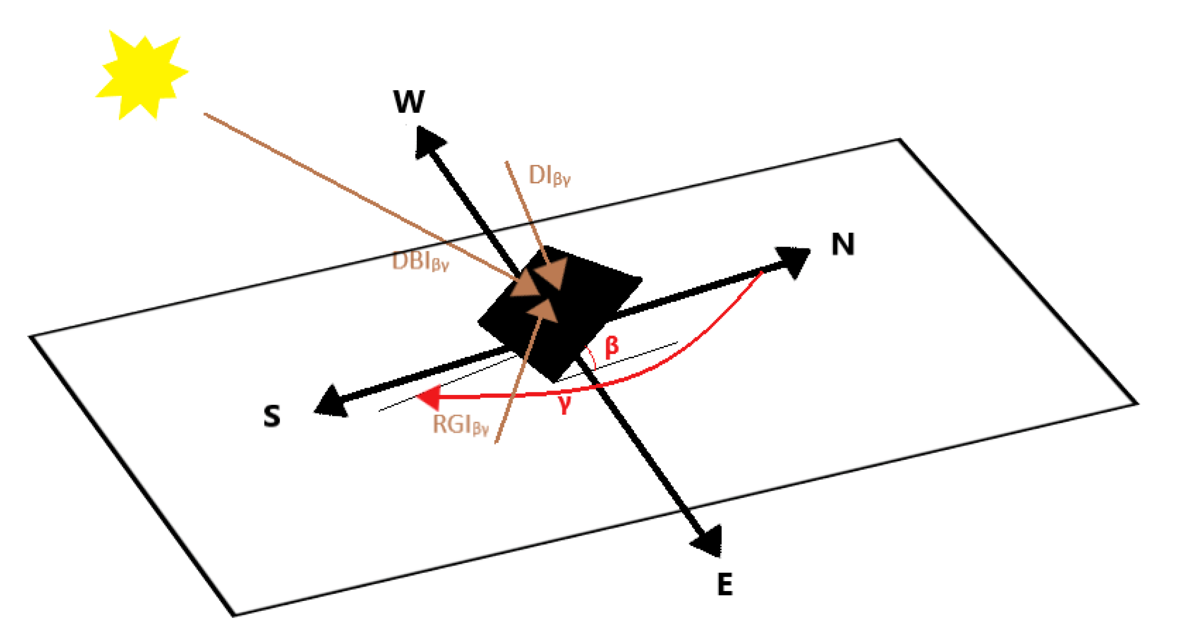
2.2. Diffuse Irradiance Models

A surface tilted at β angle and installed facing γ azimuth angle, receives Global Irradiance GIβγ, which could be analyzed to direct DBIβγ, diffuse DIβγ and reflected from the ground RGIβγ components. A graphical representation of the relations between the irradiance components is provided in Figure 2.
G I β γ = D B I β γ + D I β γ + R G I β γ
Various approaches have been suggested to model the incident GIβγ, which are estimating the diffuse component. The simplest approach is to assume that the propagation of irradiance is isotropic. Anisotropic models also consider the components of diffuse irradiance coming from circumsolar and the horizon.
Four different irradiance models have been evaluated in order to estimate the incident irradiance to inclined surfaces. These models are accordingly ISO [32], Hay [33], Reindl [34] and Perez [35]. The formulas used by these models are presented in Appendix A. The main difference between them is that ISO mοdel assumes isotropical irradiance, Hay and Reindl models also estimate irradiance from circumsolar and Perez model is the only one adding diffuse irradiance from the horizon. Four cities (Nicosia, Athens, Bergen and Reykjavik) were selected to perform the evaluation in the whole dataset.
We are not aware of any available ground-based measurements at different tilt angles in order to validate the results. A similar study performed in Athens [8] showed very small deviations between the results, with Hay showing the best agreement with tilted pyranometers. Other studies [36,37], found the Perez model to outperform the others in Reunion island and Denmark, accordingly. Chinchilla [26] suggested that Perez model had the best results when validated against BSRN stations.
Finally, the selection of the surface albedo plays a crucial role in calculating RGIβγ. For lower latitudes a constant isotropic model was used, which suggests a constant value of ρ = 0.2. Snow is the main factor that causes significant variations from the constant value. A simple approach in this case is to use an isotropic seasonal model, which changes monthly according to climatological conditions and calculated by the formula found at [38]. We have used this model for cities with latitudes higher than 50°, aiming to reduce the error introduced by snow covered conditions.

3. Results

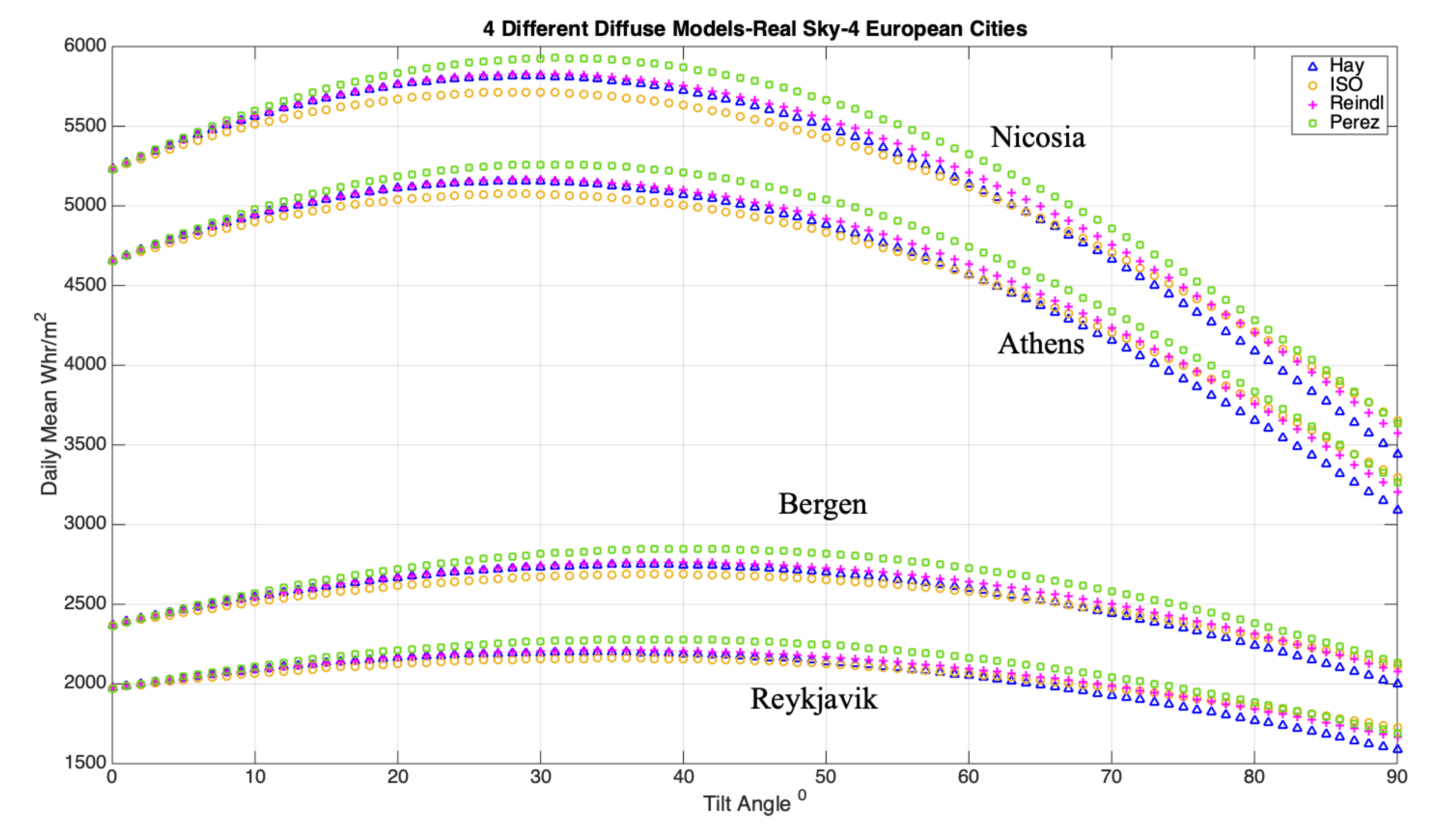
3.1. Model Comparison

In order to compare the models, we have calculated for each city the GI at tilt angles from 1° to 90° with 1° step, for all time steps. The comparison is performed for four cities, two in Southern and two in Northern Europe, in order to minimize local effects. The total estimated received energy per day, for each angle for the whole period and then the mean values are calculated. Finally, we estimated the tilt angle that had the highest daily energy outcome for each city. Results of our assessment are presented in Figure 3 and Table 1 and Table 2. Perez model estimates higher energy output than the other three models, which is partially explained by being the only one adding the horizon diffuse irradiance component. When inclination is close to 0°, the differences between the models are almost zero. This is explained by the fact that the horizontal irradiance is the main component at these inclinations, which is also the input to the models. Hay and Reindl models have almost the same results in angles lower than 60° but diverge significantly when the inclination is closest to the vertical. In addition, the ISO model estimates the lowest irradiance values, in all cases, when inclination is lower than 60°. Standard deviation of optimal angle is between 1.25° and 1.78° and the one of daily energy output 0.05–0.09 kWh/m2/day. Higher deviation of optimum angle is found in Reykjavik, where Perez model provides a more than 2° higher angle than any other model, and this should be linked with the diffuse irradiance from the horizon, which is only considered at this model. On southern latitudes models’ estimations converge on optimal tilt angle. On the other hand, in terms of absolute energy values at these latitudes the differences are higher than in Northern areas. Perez models seem to constantly provide higher irradiance compared to the others, while Hay model has the lowest values in northern areas and ISO in southern. Reindl model is the one closest to the mean value of all four models, both in terms of mean energy and optimum tilt angle, in most cases, although with very slight differences from Hay. Hence, we will use Reindl model for the rest of the study, clarifying that there is an uncertainty entered by the selection of diffuse irradiance model, in the order of 0.7° in terms of inclination angle and 0.04 kWh/m2/day in terms of energy output. This uncertainty was calculated by the mean difference of Reindl’s model to other three for all cities.

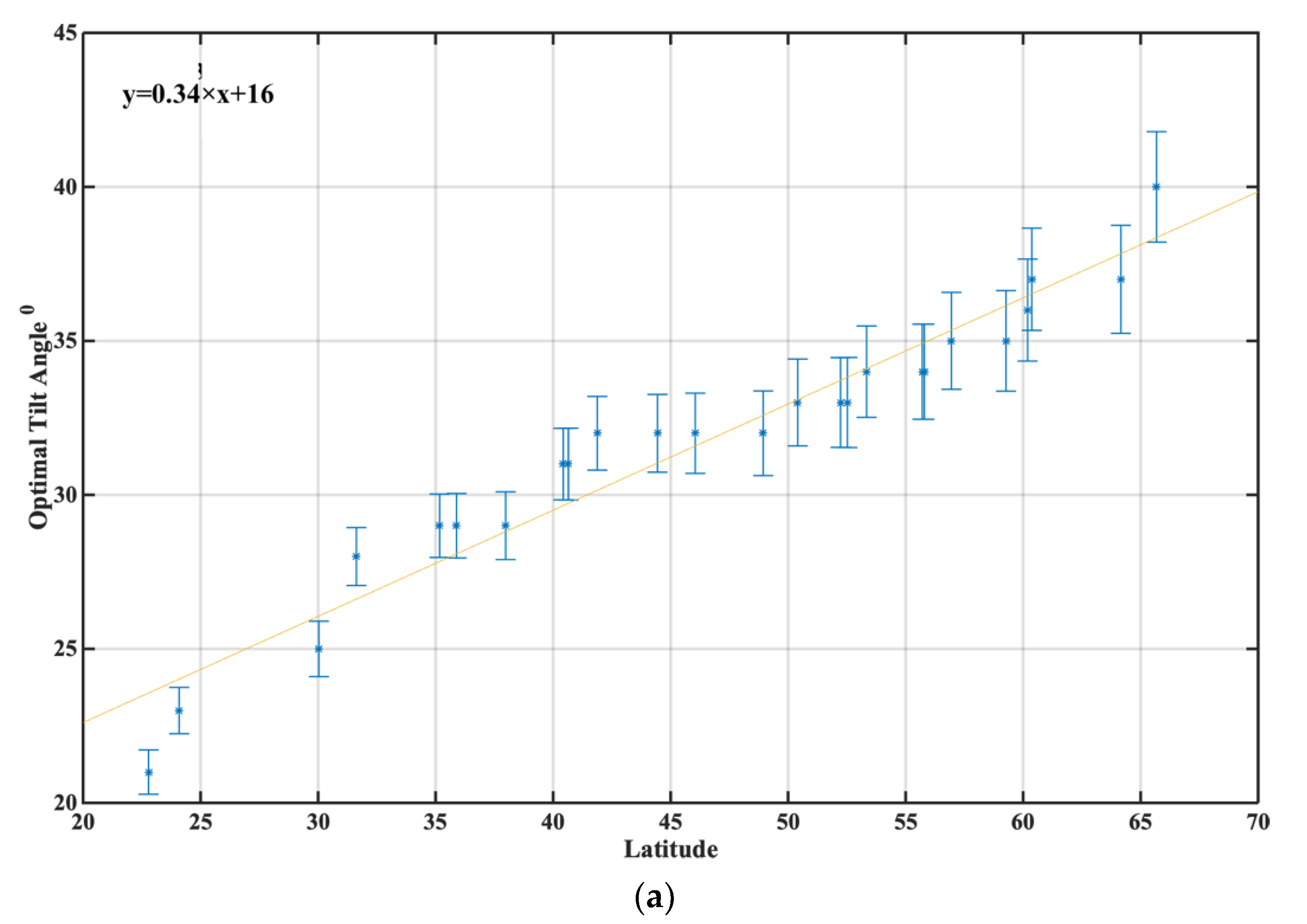
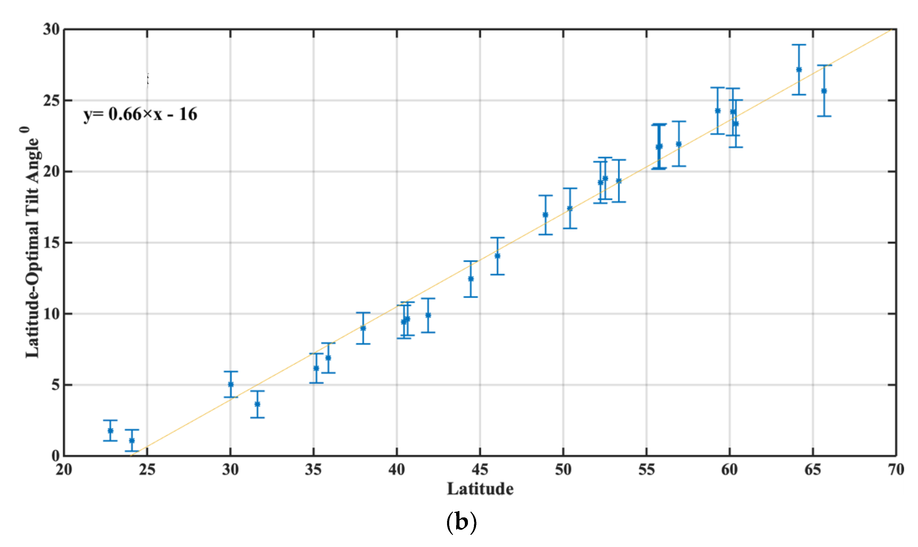
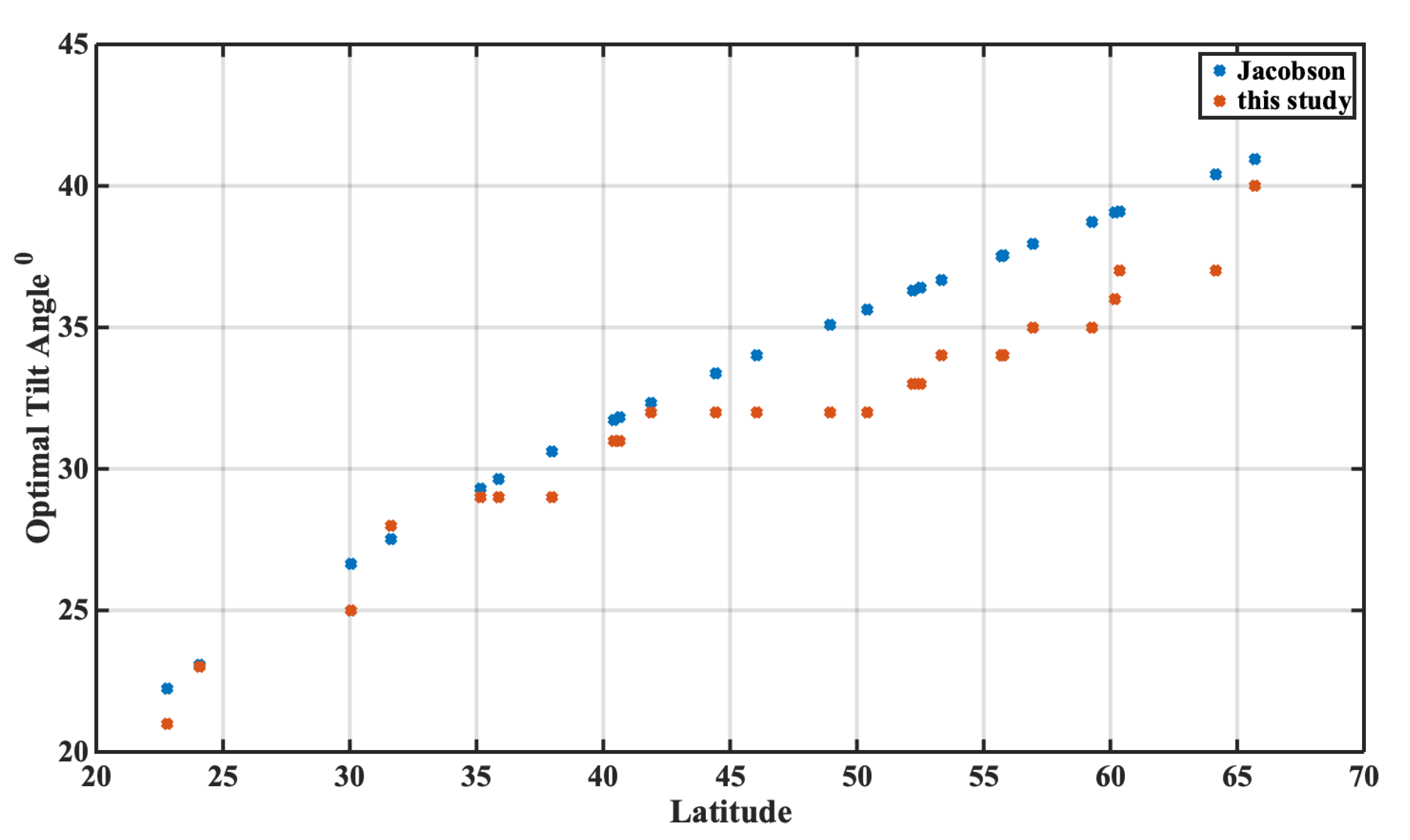
3.2. Optimum Angle per City
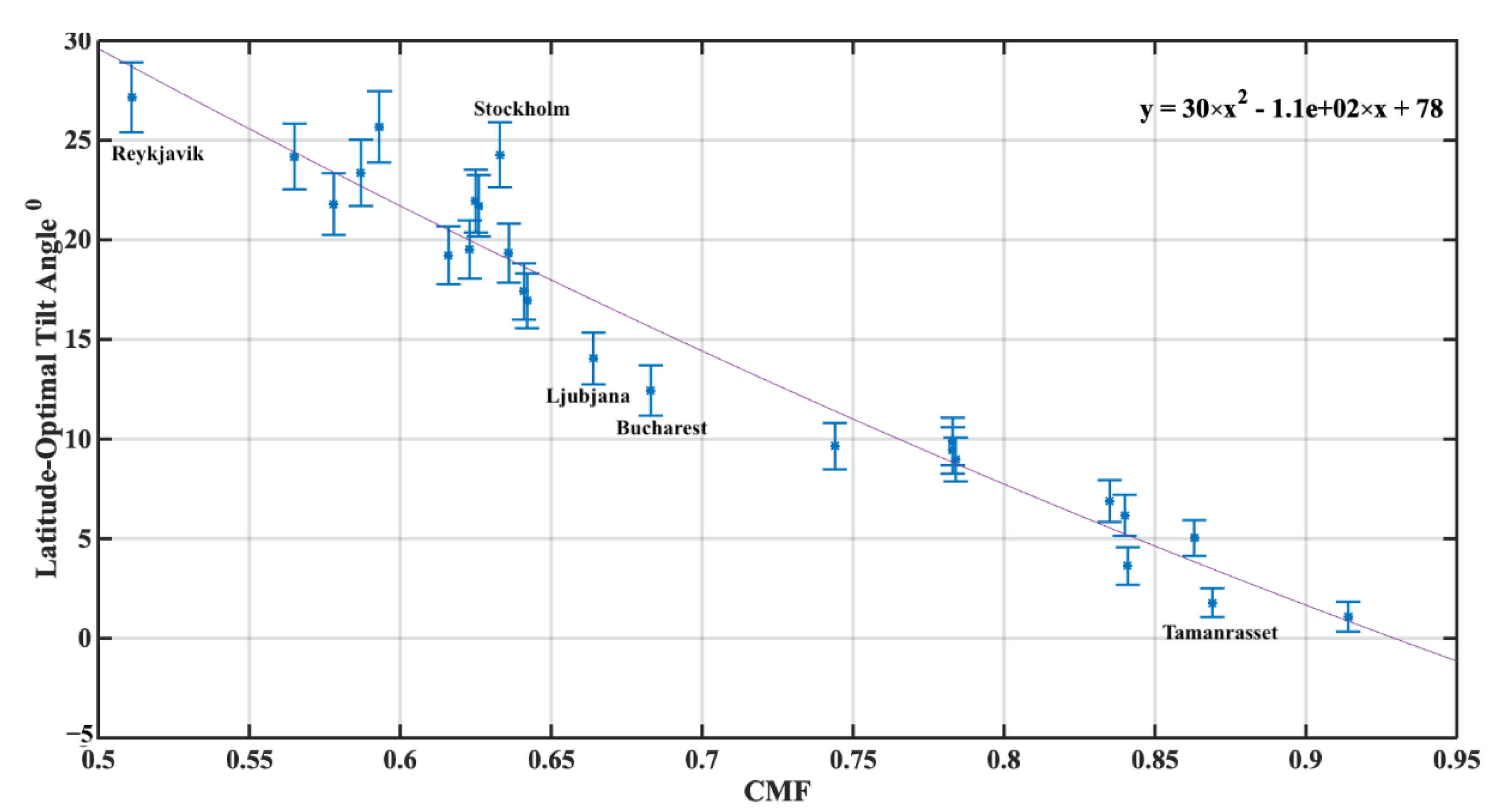
We have calculated the optimal tilt angle, that provides the highest energy outcome year-round, for each city, as estimated by the full historical hourly data. For these calculations the Reindl model has been used and the GIβ has been estimated for the whole dataset, for β in the range 1° to 90° with 1° step. Then, the sum of received irradiance at each β for the whole period, was calculated and the β with the higher value for each city was selected as optimal. The results are presented at Table 3, alongside with mean CMF and AOD at 550 nm for each city. The difference between latitude and optimal tilt angle is widen to the northern areas. This behavior should be explained mainly by the increase of cloud coverage at these areas. At southern areas, the tilt angles differences are smaller, because the latitude suggest closer to horizontal tilt and cloud coverage is lower. However, these areas receive more sunlight, hence these smaller variations could lead to significant energy gains. CMF is generally lower as latitude increases, at least in the region of Europe and North Africa. AOD on the other hand has higher values in lower latitudes in this region, which is explained by the dominance of Saharan dust on high aerosol episodes in the area [39,40].
At Figure 4, we present the mean monthly ratio between GIβ and GHI, which represents the gain/loss of tilted surface, compared with a horizontal one. Both the cases of tilt angle of latitude and the optimal as calculated above are demonstrated. In addition, monthly values for all 25 cities are implemented at the plot. In wintertime, the relative gain is higher, but also the spread of ratios among cities. In general, areas with very low cloud coverage—at southern areas—have less relative gain, although the absolute values are higher. Areas at the north, where sunshine duration is very low during winter seem to have the biggest relative benefit, since the cloud coverage is almost permanent at this season. In spring and autumn, the relative gains of optimal instead of latitude angle are more obvious. In addition, at these seasons, the relative benefit of higher latitudes is larger than the southern ones. More interesting is that in summer months, almost in all cities, both setups provide less energy than the horizontal surface. This is explained because the Solar Zenith Angle of the periods of peak GHI are closest to 0 than to latitude in all cases, hence the horizontal surface receives more irradiance. The biggest disadvantage of having a fixed angle year-round is that during summer months the solar potential is not fully exploited, but summing the whole year, it is the preferred setup. Previous work (e.g., [8]) have investigated the possibility of 2 or 4 changes of the fixed angle, around the year in order to increase the benefits.
Clouds are the main the factor that act on the propagation of radiation and alter the most efficient tilt angle. By observing that in the region of study, these are almost proportional to geographical latitude, we decided to test the possibility of using latitude as a proxy of these factors. Our aim is to extract by regression an equation that could be applied in places where no climatological information is available on clouds and aerosols. The equation should be in the form of:
βopt = f(φ)
And we have plotted optimum tilt angle (with ±1σ error bars) against the latitude for all 25 cities (Figure 5a). The linear regression forecast equation is shown on the Figure and the extracted linear polynomial is:
βopt = 0.34 × φ + 15.72
The goodness of fit is satisfactory with R2 = 0.937 and RMSE = 1.81. Hence, this equation could be in use.
But since the normal in actual installations is to use the latitude of the area as the tilt angle, we decided to parameterize an equation as the difference of the latitude and the optimum angle, in an equation of the form:
φβopt = f(φ)
Which is calculated by the corresponding plot at Figure 5b and the calculated polynomial is:
φβopt = 0.65 × φ − 15.72
In this case, the goodness of fit is better, with R2 = 0.945 and RMSE = 1.71. The quantity φβ that we parameterized, is the component of the tilt angle that is depended on atmospheric conditions, since the astronomical calculations suggest the latitude as preferred tilt angle for clear skies conditions.
We can notice in both plots that Tamanrasset has the largest distance to the regression line (~3°), which leads to doubt on applying these equations in subtropical areas. In general, with both approaches the results are adequate, keeping in mind that latitude is just a proxy of the actual conditions and that these relations could not be applied everywhere, since not all places show this latitudinal dependence—due to different cloud patterns in other regions.

3.3. Cloud Effect

In this section we aim to quantify the effect of clouds on the selection of the most efficient tilt angle. Cloud presence is the main factor that modifies the GI and makes tilt angles closer to the horizontal more efficient. Clouds effect is greater than any other atmospheric component and since aerosols and gases are included the clear sky GHI calculation, CMF calculated is an adequate measure for the effect of clouds.
At Figure 6, the relation of the difference of tilt angle in respect to CMF is shown. A parameterization in the form of:
φβopt = f(CMF)
is exported from this data set by second degree polynomial regression as:
φβopt = 30.24 × CMF2 − 112.16 × CMF + 78.12
Statistics of this fit show R2 = 0.962 and RMSE = 1.48. Thus, we should interpret that this approach is a more accurate representation of the actual state. For cities with lower cloud coverage—which are also at lower latitudes—change of tilt angle is more accurately predicted, except for Tamanrasset, where desert dust aerosols add some variation to the calculations. Bucharest and Ljubljana show lower change of the tilt angle than expected from the regression of CMF of the area. Finally, at Stockholm the actual change is more than 5° greater than predicted from the CMF equation (19.4° instead of 24.7°), where the latitude parameterization provided a more accurate estimation for the area (24.1°).
The uncertainty due to the selection of diffuse irradiance model should be considered here, since variations between them have different effect according to the actual climatological cloud properties in each area. Since, Reindl model is used, as discussed in Section 3.1, the simulation of the diffuse angle could be in the range of ±0.7° for the tilt angle. It should be highlighted that other factors for defining the optimal angle (mainly aerosols) are ignored at this approach and could be attributed for the deviations.
We have calculated the differences of mean daily energy output for areas where the simulations and the regression show large deviations. For Stockholm the difference is 0.02 kWh/m2/day, for Ljubljana is 0.04 kWh/m2/day, for Bucharest is 0.03 kWh/m2/day and for Tamanrasset is 0.01 kWh/m2/day.

3.4. Energy/Financial Profits

Figure 7 shows the energy and financial profits of the optimal tilt angle (OPT) as compared to the latitudinal tilt angle (LAT) for a 1 MWp capacity PV system, hypothetically installed in the 25 cities in Europe and North Africa. For the PV and financial calculations, the methodology described in numerous studies [41,42,43,44] was followed in brief, for the PV calculations the crystalline silicon was assumed as the most popular technology worldwide [45] accompanied by a research-cell efficiency of 13–26% [46]. By including realistic operating conditions of the PV infrastructure, the total efficiency value falls to an average level of almost 12%. The combined losses are of the order of 29% and are related to external and self-shading [47] (to avoid the self-shading a spatial coverage close to 80% is recommended for tilted panels at horizontal rooftops), as well as thermal, reflection, cables and inverter losses, but also dust and dirt deposition [48]. For the simulation of the above energy production technicalities the Photovoltaic Geographic Information System (PVGIS) was used [49]. To this direction, the cities were sorted by the corresponding solar energy potential difference between the optimal and the latitude tilt angles (blue line in Figure 7). The above solar energy potential values are translated also to percentage differences in the range of 0–2.37% (blue bars in Figure 7) indicating the overall improvement from the selection of the optimum tilt angle. The result is dependent on the average cloudiness (see Table 3) of the cities with the lowest differences occurring in the North African locations and southern Europe (e.g., Cairo, Tamanrasset, Aswan, Athens, Nicosia) and the highest differences at higher latitudes, i.e., 23 kWh/m2 in Alvsbyn (977 and 1000 kWh/m2 for latitude and optimal angles, respectively). For the estimation of the financial profit, the feed-in tariffs (FIT) retrieved from the European Environment Agency (https://www.eea.europa.eu/ (accessed on 1 April 2022)) were incorporated in the calculations, indicating the policy making dimension into the PV technology promotion and penetration into society. The above statement is reflected in the wide price range which is from 0.019 to 0.19 euro/kWh with the lowest FIT occurring in cities such as Alvsbyn, Stockholm, Copenhagen, Aswan and Cairo (<0.04 euro/kWh) and the highest prices in Madrid, Rome, Valletta, Kyiv, Warsaw and Dublin (>0.12 euro/kWh). Especially in Dublin, the revenue difference is close to 2750 euro for 1 MWp capacity on an annual basis, making the optimal angle identification a key parameter for the financial profit optimization.

4. Discussion

The validity of the results is strongly dependent on the data set used for the calculations. Historic assimilated data from CAMS database were used in this study, for 15 years. Variations in atmospheric conditions from year to year, would affect the final outcome. 15 years is a period that some outliers in cloud coverage would be detected but could only considered as representative for this time period. The pioneer work of Jacobson [24], used typical meteorological years from PVWatts database for places all over the globe, which was calculated using data from the 1960–1990 period. PVWatts uses the Bird Simple Spectral Model [50], which uses the isotropy assumption for calculating incident irradiance on titled surfaces. 10 Cities presented in that study, are common with present work (including Vatican City in Rome metropolitan area and Rabat, Malta which is located less than 10 km from Valetta). For 3 cities the exact same optimum tilt angle is estimated in Jacobson and our study and another five have differences of less than 2°. For Stockholm and Reykjavik high differences are found between the studies—6° in both cases. Factors that could explain these differences could be the different time periods for the calculations, differences in cloud conditions, the circumsolar radiation ignored by the Bird Model and the surface albedo in snow covered areas. It should be highlighted that in many areas the atmospheric pollution (including aerosols) had changed between the periods covered by PVWatts and CAMS datasets [51,52]. Additionally, the exact optimal tilt angles for all 25 cities included in the present study, were calculated using the global equation proposed by Jacobson and are shown in Figure 8. The mean difference is 1.9° with higher difference found at Reykjavik which is 3.7°. Generally, Jacobson equation estimates higher optimal angles than the ones found on this study, with the area of latitudes above 45° having the biggest deviations. This behavior is partially explained by the curvature of the 3rd order polynomial selected on Jacobson study, which deviates more at these latitudes. Nevertheless, the further north city of Alsbyn show difference of 0.9°, which is lower than other Northern cities. Cloud coverage is the reason for this behavior, since in this area, the cloud coverage is lower than other areas with latitudes above 60°. These deviations point out the difficulty of having a global parameterization for optimal tilt angle in respect to latitude, since cities with same latitude could have a large deviation in meteorological conditions and more regional scales should be preferred for these calculations. However, the parameterization in respect to cloud coverage, show a potential for application in larger scales, since it is the main variable causing the modification of the optimal angle.
Other issues that should be considered when selecting a fixed angle PV installation, such natural rain washing of dust on the panels, which is more effective at higher inclinations. Potential trends of atmospheric pollution and/or cloudiness for the next decades should be considered before selecting inclinations for PV with long lifetime. Finally, the exact financial costs of installing solar tracking systems and compared to the optimum fixed angle selection and balance the energy benefits of each solution, including the seasonality.

5. Conclusions

The preferred tilt angle for surfaces in order to maximize received solar irradiance have been studied. 25 cities in Europe and North Africa were selected and 15 years of irradiance data from CAMS were exploited. Four different diffuse irradiance models were tested, and we have selected to carry out the study using Reindl model with isotropic constant albedo at lower latitudes and isotropic seasonal albedo for regions above 50°. The uncertainty introduced by the selection of the model has been estimated as 0.7° tilt angle and 0.04 kWh/m2/day energy output.
The optimum tilt angle that provides the maximum intake of solar irradiance year-round has been estimated for each city. The difference between the latitude and the optimum tilt angle has been parameterized in respect to latitude and CMF and corresponding equations are presented in order to be applied by users in other areas. Agreement of the proposed equations—quantified as R2—was found between 0.93 and 0.97. Better statistics for the parameterization using the CMF, but with some regions having considerable differences. These equations could be employed anywhere in the same region to select the optimal tilt angle. In general, installations at higher latitudes could benefit from considerably lower tilt angle than the latitude. Higher cloud coverage also leads to optimal tilt angles closer to the horizontal. At middle latitudes the absolute differences of the tilt angles were smaller but lead to considerable energy benefits.
From an economic point of view, the selection of the optimum tilt angle is able to result in an average annual increase in revenue reaching almost 2800 euro per 1 MWp of capacity installed as compared to the latitudinal tilt. At the same time, the national strategies concerning the running feed-in tariffs form a critical parameter that affects the revenue streams depending on solar energy production and the subsequent profitability margins.
Differences from the global equation for optimal tilt angle proposed by Jacobson [24] were investigated and found that the equation overestimates more than 2° in European regions with latitude higher than 45°. Reasons for those deviations are found in the selection of different models and training datasets.
When planning new PV installations, it is rare to have years long ground-based measurements of solar irradiance in the area. In most cases databases such as CAMS or PVWatts are the best tool available, but it should be considered that they are reanalysis models based on historical satellite retrievals, hence it differs from actual solar measurements. However, studies [53,54,55] showed that these differences can be considered reasonable with no systematic deviations related with latitude. These tools are the proper way to approach the prognosis for the optimal tilt angle in a region for the next decades.
In summary, when considering fixed tilt installations, the cloud (and aerosol) climatology of the area should be taken into account alongside with estimations for the next decades. Small variations of datasets or tools used, could lead to high financial gains/loses. Future research should focus on the homogenization of the procedures in order to provide accurate and accessible tools to anyone planning to exploit solar energy potential.

Author Contributions

Conceptualization, I.-P.R. and S.K.; methodology, I.-P.R., S.K. and P.K.; software, A.M. and I.-P.R.; formal analysis, A.M. and I.-P.R.; investigation, A.M., I.-P.R. and P.K.; resources, S.K.; data curation, A.M. and I.-P.R.; writing—original draft preparation, I.-P.R. and P.K.; writing—review and editing, S.K. and P.K.; visualization, A.M., P.K. and I.-P.R.; supervision, S.K. and I.-P.R.; funding acquisition, S.K. All authors have read and agreed to the published version of the manuscript.

Funding

This research received no external funding.

Data Availability Statement

All CAMS data are available freely for download Copernicus portal http://atmosphere.copernicus.eu/ (accessed on 1 April 2022) and the SODA portal http://www.soda-pro.com/web-services/radiation/cams-radiation-service (accessed on 1 April 2022).

Acknowledgments

We acknowledge the support of European Commission project EuroGEO e-shape (grant agreement No. 820852) and by the Eiffel project (grant agreement No. 101003518).

Conflicts of Interest

The authors declare no conflict of interest.

Appendix A

Relations used for calculating in:
ISO
D I β γ I S O = D H I · ( 1 + c o s β ) 2    
Hay
D I β γ H A Y = D H I · [ ( 1 B H I I 0 ) · ( 1 + c o s β ) 2 + B H I I 0 · cos ( θ ) cos ( θ z ) ]
Reindl
D I β γ R e i n d l = D H I · [ ( 1 B H I I 0 ) · ( 1 + c o s β ) 2 · ( 1 + f · s i n 3 ( β 2 ) ) + ( B H I I 0 · cos ( θ ) cos ( θ z ) ) ]
f = 1 ( D H I G H I ) 2
Perez
D I β γ P E R E Z = D H I · [ ( 1 F 1 ) · ( 1 + c o s β 2 ) + F 1 · ( α 0 α 1 ) + F 2 · s i n β ]
where α0 and α1 are calculated as:
α 0 = m a x [ 0 , c o s θ ]
α 1 = m a x [ c o s 85 , c o s θ z ]
F1 and F2 are estimated by parameter ε and Δ as:
F 1 = m a x [ 0 , F 11 + F 12 · Δ + ( π / 180 ) · θ z · F 13 ]
F 2 = [ F 11 + F 22 · Δ + ( π / 180 ) · θ z · F 23 ]
where:
Δ = m · D H I I 0
m = 1 sin ( E l ) + a ( E l + b ) c
El is solar elevation (°) and a, b, c are constants, used as 0.15, 3.885, 1.253. Clarity index ε is calculated:
ε i = ( D H I + D N I D H I ) + 5.535 · 10 6 · θ z 3 1 + 5.535 · 10 6 · θ Ζ 3
where θΖ.
Through ε and the table provided at [33] the parameters F11, F12, F13, F22, F23 are calculated and finally the diffuse irradiance DIβγPerez.

References

  1. Malm, A. Fossil Capital: The Rise of Steam-Power and the Roots of Global Warming; Verso: London, UK; New York, NY, USA, 2016; ISBN 978-1-78478-129-3. [Google Scholar]
  2. Kåberger, T. Progress of Renewable Electricity Replacing Fossil Fuels. Glob. Energy Interconnect. 2018, 1, 48–52. [Google Scholar] [CrossRef]
  3. Shukla, P.R.; Skea, J.; Slade, R.; Al Khourdajie, A.; van Diemen, R.; McCollum, D.; Pathak, P.; Some, S.; Vyas, P.; Fradera, R.; et al. IPCC, 2022: Climate Change 2022: Mitigation of Climate Change. In Contribution of Working Group III to the Sixth Assessment Report of the Intergovernmental Panel on Climate Change; IPCC: Geneva, Switzerland, 2022. [Google Scholar]
  4. Renewables Global Futures Report: Great Debates towards 100% Renewable Energy; REN21: Paris, France, 2017.
  5. IEA (2021), Renewables 2021. Available online: https://www.iea.org/reports/renewables-2021 (accessed on 1 May 2022).
  6. Mehleri, E.D.; Zervas, P.L.; Sarimveis, H.; Palyvos, J.A.; Markatos, N.C. Determination of the Optimal Tilt Angle and Orientation for Solar Photovoltaic Arrays. Renew. Energy 2010, 35, 2468–2475. [Google Scholar] [CrossRef]
  7. Kaldellis, J.; Zafirakis, D. Experimental Investigation of the Optimum Photovoltaic Panels’ Tilt Angle during the Summer Period. Energy 2012, 38, 305–314. [Google Scholar] [CrossRef]
  8. Raptis, P.I.; Kazadzis, S.; Psiloglou, B.; Kouremeti, N.; Kosmopoulos, P.; Kazantzidis, A. Measurements and Model Simulations of Solar Radiation at Tilted Planes, towards the Maximization of Energy Capture. Energy 2017, 130, 570–580. [Google Scholar] [CrossRef]
  9. Kocer, A.; Yaka, I.F.; Sardogan, G.T.; Gungor, A. Effects of Tilt Angle on Flat-Plate Solar Thermal Collector Systems. Curr. J. Appl. Sci. Technol. 2015, 9, 77–85. [Google Scholar] [CrossRef]
  10. Tong, X.; Sun, Z.; Sigrimis, N.; Li, T. Energy Sustainability Performance of a Sliding Cover Solar Greenhouse: Solar Energy Capture Aspects. Biosyst. Eng. 2018, 176, 88–102. [Google Scholar] [CrossRef]
  11. Kacira, M.; Simsek, M.; Babur, Y.; Demirkol, S. Determining Optimum Tilt Angles and Orientations of Photovoltaic Panels in Sanliurfa, Turkey. Renew. Energy 2004, 29, 1265–1275. [Google Scholar] [CrossRef]
  12. Lave, M.; Kleissl, J. Optimum Fixed Orientations and Benefits of Tracking for Capturing Solar Radiation in the Continental United States. Renew. Energy 2011, 36, 1145–1152. [Google Scholar] [CrossRef] [Green Version]
  13. Rowlands, I.H.; Kemery, B.P.; Beausoleil-Morrison, I. Optimal Solar-PV Tilt Angle and Azimuth: An Ontario (Canada) Case-Study. Energy Policy 2011, 39, 1397–1409. [Google Scholar] [CrossRef]
  14. Díez-Mediavilla, M.; Rodríguez-Amigo, M.; Dieste-Velasco, M.; García-Calderón, T.; Alonso-Tristán, C. The PV Potential of Vertical Façades: A Classic Approach Using Experimental Data from Burgos, Spain. Sol. Energy 2019, 177, 192–199. [Google Scholar] [CrossRef]
  15. Wang, M.; Mao, X.; Gao, Y.; He, F. Potential of Carbon Emission Reduction and Financial Feasibility of Urban Rooftop Photovoltaic Power Generation in Beijing. J. Clean. Prod. 2018, 203, 1119–1131. [Google Scholar] [CrossRef]
  16. Mohammad, S.T.; Al-Kayiem, H.H.; Aurybi, M.A.; Khlief, A.K. Measurement of Global and Direct Normal Solar Energy Radiation in Seri Iskandar and Comparison with Other Cities of Malaysia. Case Stud. Therm. Eng. 2020, 18, 100591. [Google Scholar] [CrossRef]
  17. Nassar, Y.F.; Hafez, A.A.; Alsadi, S.Y. Multi-Factorial Comparison for 24 Distinct Transposition Models for Inclined Surface Solar Irradiance Computation in the State of Palestine: A Case Study. Front. Energy Res. 2020, 7, 163. [Google Scholar] [CrossRef]
  18. Serrano-Guerrero, X.; Cantos, E.; Feijoo, J.-J.; Barragán-Escandón, A.; Clairand, J.-M. Optimal Tilt and Orientation Angles in Fixed Flat Surfaces to Maximize the Capture of Solar Insolation: A Case Study in Ecuador. Appl. Sci. 2021, 11, 4546. [Google Scholar] [CrossRef]
  19. Darhmaoui, H.; Lahjouji, D. Latitude based model for tilt angle optimization for solar collectors in the Mediterranean region. Energy Procedia 2013, 42, 426–435. [Google Scholar] [CrossRef] [Green Version]
  20. Chang, Y.-P. Optimal Design of Discrete-Value Tilt Angle of PV Using Sequential Neural-Network Approximation and Orthogonal Array. Expert Syst. Appl. 2009, 36, 6010–6018. [Google Scholar] [CrossRef]
  21. Nicolás-Martín, C.; Santos-Martín, D.; Chinchilla-Sánchez, M.; Lemon, S. A Global Annual Optimum Tilt Angle Model for Photovoltaic Generation to Use in the Absence of Local Meteorological Data. Renew. Energy 2020, 161, 722–735. [Google Scholar] [CrossRef]
  22. Salata, F.; Ciancio, V.; Dell’Olmo, J.; Golasi, I.; Palusci, O.; Coppi, M. Effects of Local Conditions on the Multi-Variable and Multi-Objective Energy Optimization of Residential Buildings Using Genetic Algorithms. Appl. Energy 2020, 260, 114289. [Google Scholar] [CrossRef]
  23. Petrović, E.; Jović, M.; Nikolić, V.; Mitrović, D.; Laković, M. Particle Swarm Optimization for the Optimal Tilt Angle of Solar Collectors. In Proceedings of the Sixteenth Symposium on Thermal Science and Engineering of Serbia, Sokobanja, Serbia, 22–25 October 2013. [Google Scholar]
  24. Jacobson, M.Z.; Jadhav, V. World Estimates of PV Optimal Tilt Angles and Ratios of Sunlight Incident upon Tilted and Tracked PV Panels Relative to Horizontal Panels. Sol. Energy 2018, 169, 55–66. [Google Scholar] [CrossRef]
  25. NREL (National Renewable Energy Laboratory), 2017. PV Watts Calculator. Available online: http://Pvwatts.Nrel.Gov (accessed on 4 November 2017).
  26. Chinchilla, M.; Santos-Martín, D.; Carpintero-Rentería, M.; Lemon, S. Worldwide Annual Optimum Tilt Angle Model for Solar Collectors and Photovoltaic Systems in the Absence of Site Meteorological Data. Appl. Energy 2021, 281, 116056. [Google Scholar] [CrossRef]
  27. Oumbe, A.; Qu, Z.; Blanc, P.; Lefèvre, M.; Wald, L.; Cros, S. Decoupling the Effects of Clear Atmosphere and Clouds to Simplify Calculations of the Broadband Solar Irradiance at Ground Level. Geosci. Model Dev. 2014, 7, 1661–1669. [Google Scholar] [CrossRef] [Green Version]
  28. de Miguel, A.; Bilbao, J.; Aguiar, R.; Kambezidis, H.; Negro, E. Diffuse Solar Irradiation Model Evaluation in the North Mediterranean Belt Area. Sol. Energy 2001, 70, 143–153. [Google Scholar] [CrossRef]
  29. Kopp, G.; Lean, J.L. A new, lower value of total solar irradiance: Evidence and climate significance. Geophys. Res. Lett. 2011, 38. [Google Scholar] [CrossRef] [Green Version]
  30. Parisi, A.V.; Turnbull, D.J.; Turner, J. Calculation of cloud modification factors for the horizontal plane eye damaging ultraviolet radiation. Atmos. Res. 2007, 86, 278–285. [Google Scholar] [CrossRef]
  31. Lefèvre, M.; Oumbe, A.; Blanc, P.; Espinar, B.; Gschwind, B.; Qu, Z.; Wald, L.; Schroedter-Homscheidt, M.; Hoyer-Klick, C.; Arola, A.; et al. McClear: A New Model Estimating Downwelling Solar Radiation at Ground Level in Clear-Sky Conditions. Atmos. Meas. Tech. 2013, 6, 2403–2418. [Google Scholar] [CrossRef] [Green Version]
  32. Liu, B.; Jordan, R. Daily Insolation on Surfaces Tilted towards Equator. ASHRAE J. 1961, 10. [Google Scholar]
  33. Hay, J.E. Calculation of Monthly Mean Solar Radiation for Horizontal and Inclined Surfaces. Sol. Energy 1979, 23, 301–307. [Google Scholar] [CrossRef]
  34. Reindl, D.T.; Beckman, W.A.; Duffie, J.A. Evaluation of Hourly Tilted Surface Radiation Models. Sol. Energy 1990, 45, 9–17. [Google Scholar] [CrossRef]
  35. Perez, R.; Ineichen, P.; Seals, R.; Michalsky, J.; Stewart, R. Modeling Daylight Availability and Irradiance Components from Direct and Global Irradiance. Sol. Energy 1990, 44, 271–289. [Google Scholar] [CrossRef] [Green Version]
  36. David, M.; Lauret, P.; Boland, J. Evaluating Tilted Plane Models for Solar Radiation Using Comprehensive Testing Procedures, at a Southern Hemisphere Location. Renew. Energy 2013, 51, 124–131. [Google Scholar] [CrossRef] [Green Version]
  37. Tian, Z.; Perers, B.; Furbo, S.; Fan, J.; Deng, J.; Dragsted, J. A Comprehensive Approach for Modelling Horizontal Diffuse Radiation, Direct Normal Irradiance and Total Tilted Solar Radiation Based on Global Radiation under Danish Climate Conditions. Energies 2018, 11, 1315. [Google Scholar] [CrossRef] [Green Version]
  38. Gueymard, C. Critical Analysis and Performance Assessment of Clear Sky Solar Irradiance Models Using Theoretical and Measured Data. Sol. Energy 1993, 51, 121–138. [Google Scholar] [CrossRef]
  39. Gkikas, A.; Proestakis, E.; Amiridis, V.; Kazadzis, S.; Di Tomaso, E.; Marinou, E.; Hatzianastassiou, N.; Kok, J.F.; García-Pando, C.P. Quantification of the Dust Optical Depth across Spatiotemporal Scales with the MIDAS Global Dataset (2003–2017). Atmos. Chem. Phys. 2022, 22, 3553–3578. [Google Scholar] [CrossRef]
  40. Papachristopoulou, K.; Fountoulakis, I.; Gkikas, A.; Kosmopoulos, P.G.; Nastos, P.T.; Hatzaki, M.; Kazadzis, S. 15-Year Analysis of Direct Effects of Total and Dust Aerosols in Solar Radiation/Energy over the Mediterranean Basin. Remote Sens. 2022, 14, 1535. [Google Scholar] [CrossRef]
  41. Kosmopoulos, P.; Kazadzis, S.; El-Askary, H.; Taylor, M.; Gkikas, A.; Proestakis, E.; Kontoes, C.; El-Khayat, M. Earth-Observation-Based Estimation and Forecasting of Particulate Matter Impact on Solar Energy in Egypt. Remote Sens. 2018, 10, 1870. [Google Scholar] [CrossRef] [Green Version]
  42. Fountoulakis, I.; Kosmopoulos, P.; Papachristopoulou, K.; Raptis, I.-P.; Mamouri, R.-E.; Nisantzi, A.; Gkikas, A.; Witthuhn, J.; Bley, S.; Moustaka, A.; et al. Effects of Aerosols and Clouds on the Levels of Surface Solar Radiation and Solar Energy in Cyprus. Remote Sens. 2021, 13, 2319. [Google Scholar] [CrossRef]
  43. Dumka, U.C.; Kosmopoulos, P.G.; Ningombam, S.S.; Masoom, A. Impact of Aerosol and Cloud on the Solar Energy Potential over the Central Gangetic Himalayan Region. Remote Sens. 2021, 13, 3248. [Google Scholar] [CrossRef]
  44. Dumka, U.C.; Kosmopoulos, P.G.; Patel, P.N.; Sheoran, R. Can Forest Fires Be an Important Factor in the Reduction in Solar Power Production in India? Remote Sens. 2022, 14, 549. [Google Scholar] [CrossRef]
  45. International Renewable Energy Agency. Future of Solar PV. 2019. Available online: https://irena.org/-/media/Files/IRENA/Agency/Publication/2019/Nov/IRENA_Future_of_Solar_PV_2019.pdf (accessed on 18 June 2022).
  46. National Renewable Energy Laboratory. Best Research-Cell Efficiency Chart. 2022. Available online: https://www.nrel.gov/pv/cell-efficiency.html (accessed on 18 June 2022).
  47. Arias-Rosales, A.; LeDuc, P.R. Shadow modeling in urban environments for solar harvesting devices with freely defined positions and orientations. Renew. Sustain. Energy Rev. 2022, 164, 112522. [Google Scholar] [CrossRef]
  48. Rao, A.; Pillai, R.; Mani, M.; Ramamurthy, P. Influence of dust deposition on photovoltaic panel performance. Energy Procedia 2014, 54, 690–700. [Google Scholar] [CrossRef] [Green Version]
  49. PVGIS. Photovoltaic Geographical Information System. Available online: http://re.jrc.ec.europa.eu/pvgis/ (accessed on 18 June 2022).
  50. Bird, R.E.; Riordan, C. Simple Solar Spectral Model for Direct and Diffuse Irradiance on Horizontal and Tilted Planes at the Earth’s Surface for Cloudless Atmospheres. J. Appl. Meteorol. Climatol. 1986, 25, 87–97. [Google Scholar] [CrossRef] [Green Version]
  51. Wild, M. Global Dimming and Brightening: A Review. J. Geophys. Res. Atmos. 2009, 114, D00D16. [Google Scholar] [CrossRef] [Green Version]
  52. Leibensperger, E.M.; Mickley, L.J.; Jacob, D.J.; Chen, W.-T.; Seinfeld, J.H.; Nenes, A.; Adams, P.J.; Streets, D.G.; Kumar, N.; Rind, D. Climatic Effects of 1950–2050 Changes in US Anthropogenic Aerosols—Part 1: Aerosol Trends and Radiative Forcing. Atmos. Chem. Phys. 2012, 12, 3333–3348. [Google Scholar] [CrossRef] [Green Version]
  53. Inness, A.; Ades, M.; Agustí-Panareda, A.; Barré, J.; Benedictow, A.; Blechschmidt, A.-M.; Dominguez, J.J.; Engelen, R.; Eskes, H.; Flemming, J.; et al. The CAMS Reanalysis of Atmospheric Composition. Atmos. Chem. Phys. 2019, 19, 3515–3556. [Google Scholar] [CrossRef] [Green Version]
  54. Gueymard, C.A.; Yang, D. Worldwide Validation of CAMS and MERRA-2 Reanalysis Aerosol Optical Depth Products Using 15 Years of AERONET Observations. Atmos. Environ. 2020, 225, 117216. [Google Scholar] [CrossRef]
  55. Mortier, A.; Gliß, J.; Schulz, M.; Aas, W.; Andrews, E.; Bian, H.; Chin, M.; Ginoux, P.; Hand, J.; Holben, B.; et al. Evaluation of Climate Model Aerosol Trends with Ground-Based Observations over the Last 2 Decades—An AeroCom and CMIP6 Analysis. Atmos. Chem. Phys. 2020, 20, 13355–13378. [Google Scholar] [CrossRef]
Figure 1. Locations of the Cities in Europe and North Africa selected for the study.
Energies 15 04784 g001
Figure 2. Graphical Presentation of the β tilt angle and γ azimuthal angle, alongside of Diffuse, Direct Beam and Reflective components of received solar irradiance.
Energies 15 04784 g002
Figure 3. Mean Daily Total Radiation for Athens, Nicosia, Bergen and Reykjavik, for inclinations of 0° to 90° as calculated by different models.
Energies 15 04784 g003
Figure 4. Ratio of GIβ on inclined surface to horizontal one, for each month. Mean value for each month for β = Latitude and β = optimum angle, along with error bars representing the 1σ standard deviation of ratios for each month. Small points are all 25 cities ratios for each month.
Energies 15 04784 g004
Figure 5. Optimum tilt angle with 1σ against latitude for all cities and corresponding linear regression (a). Difference of Latitude and Optimum tilt angle with 1 σ against latitude for all cities and corresponding linear regression (b).
Energies 15 04784 g005aEnergies 15 04784 g005b
Figure 6. Optimum tilt angle with 1 σ against latitude for all cities and corresponding linear regression.
Energies 15 04784 g006
Figure 7. Annual solar energy potential and revenue (for 1 MWp capacity) differences and percentage differences for all cities included in the study, between latitude and optimum tilt angle installations.
Energies 15 04784 g007
Figure 8. Optimal Tilt angle for the 25 Cities used in the present study, as calculated by Reindl model [31] (red) and as estimated by the equation proposed by Jacobson [24] (blue).
Energies 15 04784 g008
Table 1. Mean Optimum Angle for test cities as calculated with each model, the mean and standard deviation σ for each city as calculated from model’s prognosis.
Optimum Angle HayISOReindlPerezMeanσ
Nicosia28.828.4729.6731.2729.551.25
Athens28.3328.2729.1330.8729.151.21
Bergen37.0738.1338.840.4038.601.40
Reykjavik33.5335.2735.6737.8735.591.78
Table 2. Daily Energy outcome at the suggested optimum tilt angle for test cities as calculated with each model, the mean and standard deviation σ for each city as calculated from model’s prognosis.
kWh/m2/Day HayISOReindlPerezMeanσ
Nicosia5.815.715.835.935.820.09
Athens5.155.085.175.265.170.07
Bergen2.752.692.762.852.760.07
Reykjavik2.202.162.212.282.210.05
Table 3. Latitude and Longitude of Cities used in the study, alongside with mean CMF and AOD and the calculated optimum tilt angle β for the period 2005–2019.
CityCountryLatLongβopt<CMF><AOD>
TamanrassetAlgeria22.785.51210.8690.312
AswanEgypt24.0932.89230.9140.310
CairoEgypt30.0331.24250.8630.282
MarrakeshMorocco31.63−7.98280.8410.205
NicosiaCyprus35.1733.36290.8400.245
VallettaMalta35.8914.51290.8350.238
AthensGreece37.9823.72290.7840.222
MadridSpain40.43−3.70310.7830.140
ThessalonikiGreece40.6522.92310.7440.232
RomeItaly41.8812.47320.7830.197
BucharestRomana44.4426.08320.6830.224
LjubljanaSlovenia46.0514.50320.6640.196
ParisFrance48.942.41320.6420.178
KyivUkraine50.413050330.6410.190
WarsawPoland52.2321.00330.6160.192
BerlinGermany52.5213.37330.6230.180
DublinIreland53.34−6.28340.6360.170
CopenhagenDenmark55.7112.54340.6260.161
MoscowMoscow55.837.59340.5780.176
RigaLithuania56.9524.11350.6250.158
StockholmSweden59.2718.02350.6330.137
HelsinkiFinland60.1924.93360.5650.137
BergenNorway60.375.32370.5870.145
ReykjavikIceland64.16−21.95370.5110.138
AlvsbynNorway65.6820.99400.5930.101
Publisher’s Note: MDPI stays neutral with regard to jurisdictional claims in published maps and institutional affiliations.

