Method for Planning, Optimizing, and Regulating EV Charging Infrastructure

Abstract

The paper presents and solves the problems of modeling and designing the required EV charging service capacity for systems with a slow dynamic component. This includes possible bursts within a peak hour interval. A simulation tool with a newly implemented capacity planning method has been developed and implemented for these needs. The method can be used for different system simulations and simultaneously for systems with high, medium, and low service dynamics. The proposed method is based on a normal distribution, a primary mechanism that describes events within a daily interval (24 h) or a peak hour interval (rush hour). The goal of the presented approach, including the proposed method, is to increase the level and quality of the EV charging service system. The near-optimal solution with the presented method can be found manually by changing the service capacity parameter concerning the criterion function. Manual settings limit the number of rejected events, the time spent in the queue, and other service system performance parameters. In addition to manual search for near-optimal solutions, the method also provides automatic search by using the automation procedure of simulation runs and increasing/decreasing the service capacity parameter by a specifically calculated amount.

1. Introduction

Environmental awareness and the energy crisis are two main reasons for the revival and rise of the electric vehicle (EV) industry. Though electric mobility is still relatively new, the development of electric vehicles and charging infrastructures has been in full swing recently. There is a strong correlation between the two. An adequate charging infrastructure is necessary and relevant for EVs to succeed and thrive on the market. Public charging infrastructure that allows EV users to recharge their vehicles quickly and comfortably is critical to enabling EV adoption on a large scale [1,2]. The process of building a network of EV charging stations is complex and costly. Several conditions must be met simultaneously for an EV charging station to be economically justified at a specific location. The essential requirement for an EV charging station is the user’s need, followed by the availability of infrastructures, such as electricity distribution infrastructure, roads, and municipal infrastructure. Those conditions lead to selecting the most appropriate technology for the EV charging station. It must satisfy the widest circle of potential users in terms of its functionality and, simultaneously, be as affordable as possible. A variety of EV charging stations are available on the market, from simple and inexpensive AC versions to high-performance, fast DC charging stations.

The diversity of EV charging stations is increased by numerous solutions in EV vehicles, such as various power connectors, different AC/DC and DC/DC converters, and other technical details [3,4,5,6], further complicating the planning of EV networks. Due to the interdependence of EV charging infrastructure and the widespread use of EVs, the construction of EV charging stations in local communities has been heavily subsidized in many countries, particularly in the EU. Certainly, the measure encourages the use of EVs. However, laying EV infrastructure in the environment can have negative consequences, such as location inadequacy, technical-performance inadequacy, under-capacity, and over-capacity. In light of what was discussed above, the article investigated primarily the over-capacity and under-capacity problems of the EV charging infrastructure. The research focused on analyzing the use and determination of the optimal use of EV charging infrastructure based on the quantity and demand of potential users. Technical and performance differences between different versions of EV charging stations were excluded in the research, so the proposed method is agnostic from this perspective.

Planning the required capacity of service systems is described in various research studies [7,8,9,10,11]. Planning capacity is a strategic process of finding optimal solutions depending on the available resources and current business requirements to ensure the highest possible level of service quality, taking into account the factor of cost minimization. It is a critical and sensitive process, closely connected to capacity management, service level management, and the so-called configuration management or configuration administration [12,13,14].

Capacity planning in information technology is the science and art of estimating future requirements for space resources, computer hardware, software, and connectivity infrastructure [15]. We use capacity planning in various fields, such as energy consumption, hardware resources, hardware capacity planning [16,17], road capacity planning, business cost planning, human resource planning [18], etc. By using the planning methods, we can plan higher utilization of the existing equipment and look for ways or features with which we can influence reduction and optimization. This way, we can look for solutions for unimplemented (inexistent) systems, which are only in the phase of planning [8]. With the acquired planning solutions (depending on the accuracy of the solution—the use of an appropriate method), we can relatively quickly answer whether the chosen solution will fulfill our needs, to what degree, and in what scope is an investment rational.

The area of capacity planning and optimization [19] is a research area with specific well-known methods [7], where factors such as system dynamics, random timing of system events, and especially nonlinear relations are the primary trend of further research in this area. The listed factors are the guidelines for our proposed method, which we present in this paper. Research in this area, whether it concerns man-force planning, production capacity planning, or the suitability of processing systems planning according to the demand trends, has also been stimulated by the recent global financial crisis. People want insurance against unnecessary or wrong investments.

Nowadays, there are two approaches to capacity planning: trending capacity planning [20] and capacity modeling [7], the latter being the newer, more modern approach. Trending capacity planning uses historical patterns that include past events. In such a method, a linear trend of increasing and decreasing utilization over a period of time [21] is designed based on known patterns. An analytical prediction based on a rising and falling trend evaluates the required capacity at a given time. From this point of view, the approach is simple—its only advantage over the capacity modeling method. The disadvantage of techniques based on the linearization process is the high inaccuracy of predictions, since most events in the business world are dynamic.

Moreover, such dynamic systems also contain components of nonlinearity. The nonlinearity is particularly evident in the fluctuation of capacity according to current demand, which depends on higher-level characteristics needed at a global level. Some degree of error in a linear prediction is already inherent in the process itself. This method introduces a further error if we assume that bursts are also present in the system (random, stochastic, unforeseen, sudden loads or spikes) [22]. The consequence is an even higher level of distrust in the provided solution. The capacity modeling method is one of the modern approaches in the discussed field. Mathematical models based on statistical data, probability distributions, etc., are designed for this purpose. This model, for example, includes the information on the capacity, occupancy, and utilization of the discussed system, as they are (with no approximations, linearization, etc.). The approach enables the generation of various patterns [23,24,25], which can come from statistical data, modification of this data, or practical choice. In such an approach, we also observe the response as an output of the system (in the simulation model or the model of an observed system). In this way, we can test multiple scenarios arising from what-if questions.

Thus, the capacity modeling method allows us to predict resource demand and forecast resource provisioning according to current and future demand, always finding the near-optimal solution. Such a planning approach removes the limitations of search experiments. It enables optimal configuration, arrangement, and reorganization before rash decisions about financial investments or physical changes to a particular system [10]. This branch is the foundation for new planning solutions, as the number of possible paths or realizations for finding a suitable solution is practically unlimited. Our proposed method of planning and optimizing dynamic service system capacities is a viable solution presented in the next chapter. Existing methods (considering trends, linearizing trends, inappropriate distributions, stochastic, bursts, etc.) are insufficient and inapplicable. Hence, we developed a new solution, the applicability of which will be demonstrated using a real example of capacity planning.

We used the modeling methodology to design a dynamic planning method and optimize service capacities. Research is thus mainly devoted to this section of the work.

1.1. An Overview of the Existent Solutions

In reviewing scientific papers, we see that there are solutions of a similar nature, but they are not universal. We can compare our approach, method, methodology, and advanced tool simulator/emulator to:

• Stochastic optimal production control problem with corrective maintenance [26],
• Production planning of a hybrid manufacturing–remanufacturing system under uncertainty within a closed-loop supply chain [27],
• Intermediate storage in batch/continuous processing systems under stochastic operation [28],
• Dynamic scheduling of maintenance tasks in the petroleum industry: A reinforcement approach [29],
• The method, simulation, and analysis of necessary capacities of water supply networks depending on demand and the volume of water in the water reservoir [30],
• Method and simulation of the permeability of crossroads according to temporary traffic volume, number of lanes, the diameter of the roundabout, the randomness of exit allocation, and type of the traffic (mixed, only trucks, buses, only personal cars) [31],
• Simulator of allocation of electric charging stations in tourist centers, where electric scooters are used [32],
• Simulation as a decision tool for capacity planning [33],
• Simulation Platform for MIMO Systems [34],
• Low-Complexity MIMO Channel Simulation by Reducing the Number of Paths [35],
• Airport terminal capacity planning [36],
• Operating Room Planning with Random Surgery Times [37],
• Managing Service Capacity Under Uncertainty [38],
• Call Center Capacity Planning [39],
• Capacity Planning of Ambulance Services: Statistical Analysis, Forecasting, and Staffing [40].

A number of similar solutions exist (for example, see [17,18]); however, none of them satisfy our needs. Throughout research and method development, we strive to build a universal model and simulation scenario.

1.2. A Short Description of the Paper Structure

The paper consists of six main sections. The second section presents the components of the proposed capacity planning method, including mathematical and simulation models. The same section also includes the used optimization method and automatic analysis as an additional component of the presented optimization loop and process. The third section compares our proposed method with a reference method used for charging stations. The comparison focuses on the direct similarities and originality of both approaches. The fourth section presents statistical data used in the reference method. We also use them to directly compare the proposed method with the existing solutions and their validation. In addition, in this chapter, we present several experiments and direct comparisons to justify the suitability of the new method. The fifth section discusses experimental results and some limitations of the method. The final section summarizes the solution’s features, its applicability, and future research directions.

2. Definition of Models in the Proposed Method

The user model includes two types of users:

(1)

Users with “healthy” batteries that are more or less empty and for which a normal recharging process is performed (described with their normal distribution). Depending on the battery’s empty, the charging time varies (different charging time durations).

(2)

The so-called “lammer” users have or are about to have a battery failure. Such users stay at the EV charging station for a short period until a charge monitor electronically detects a battery failure. Such an EV is immediately removed from the charging station, which becomes free and ready to accept a new user (lammer users dramatically affect the exchange dynamics at the charging station). They are modeled similarly to real users but again with their normal distribution. The number of such users depends on the percentage of all users. Their appearance in the load pattern is completely pseudorandom.

The following three pairs of models are necessary to determine the charging capacity of an electric vehicle charging station:

(1)

‘Rush hour’ models that represent the increased/decreased user share—they provide an initial basis for stochastic patterns within the observed ‘rush hour’ where pseudorandom (see stochastic in [16,41]) localized stochastic bursts are generated;

(2)

The models as mentioned above for the lammer and real users; and

(3)

The service station capacity model.

Each model pair represents one aspect of the process T(n), such as how EVs appear in the system or are accepted into it, and another aspect of the process X(n), such as how long the charging process lasts.

As we mentioned in the introduction to this section, the user model includes two types of users. The first group consists of everyday charging system users whose vehicles have reliable batteries that are not in a state of failing or about to fail. The second group includes vehicles whose charging diagnostic system detects battery failure. The latter occupies the charging slot until the diagnostic system detects a failure. Charging takes place in this location for shorter periods than a healthy battery. Such user behavior has an influential impact on the service dynamics and the permeability of the service system. We introduced a different normal distribution in real-world charging stations for EVs, where many batteries are in a failure state or close to it. Their share can be expressed as a percentage unit of all users (EVs) in the service system. The standard deviation allows us to define time intervals within which the function randomly selects the duration of a battery’s charge or diagnosis. The system handles this by a separate thread, ensuring pseudo-randomness. For this purpose, a normal distribution function is used for lammer and real users, as was defined by [42]. 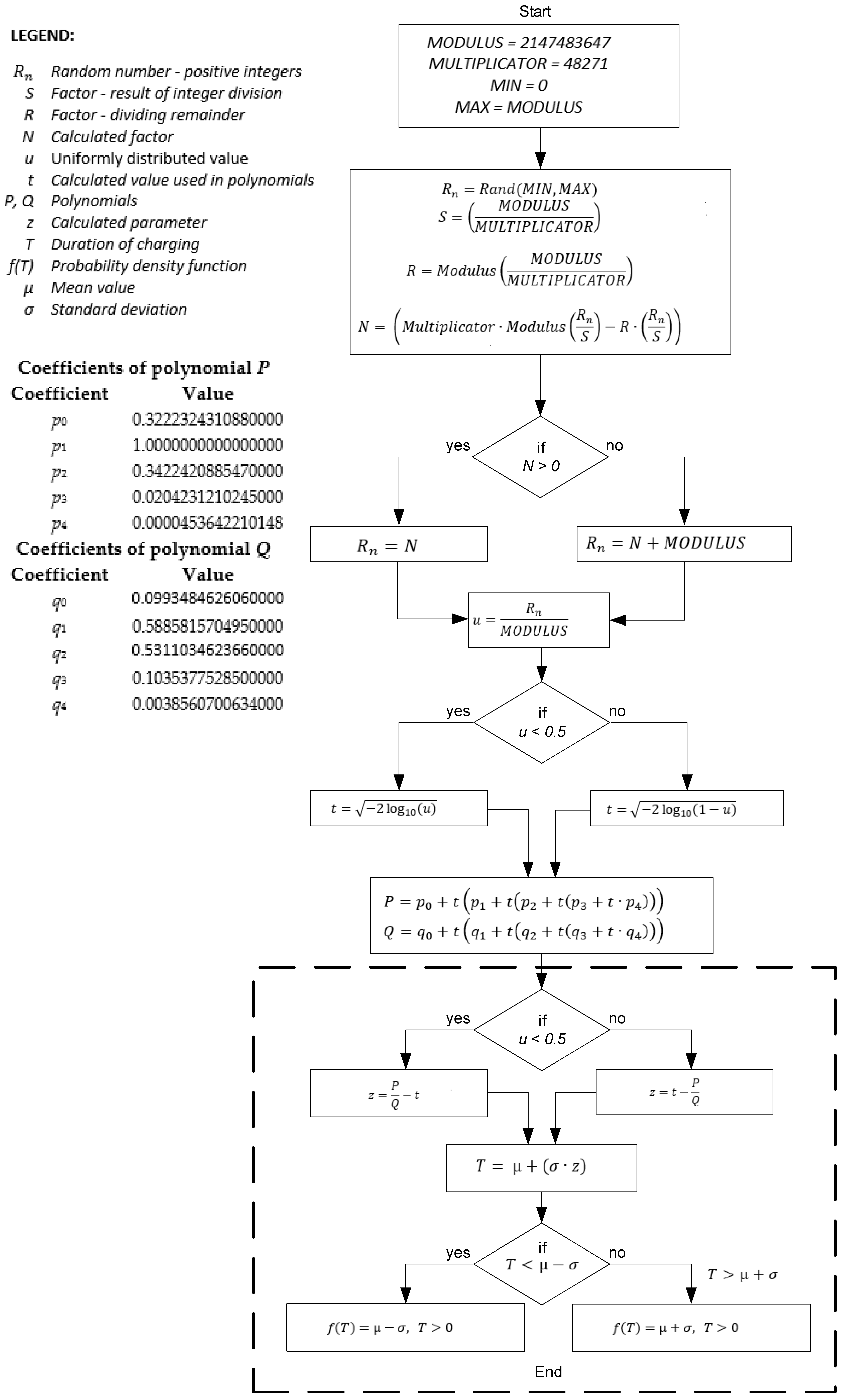Figure 1 presents a modified algorithm [42] used to model the random variable T, which represents the charging time of each EV, and calculate the probability density function f(T). In Figure 1, a dashed rectangle represents the modified part of the algorithm.

The constants MODULUS and MULTIPLICATOR, as well as the polynomials P(t) and Q(t), are the same as in [42]. An additional change has been made in calculating parameter $z\in ℝ$, which correlates to parameter u, as shown in Figure 1 in the dashed square. The duration of charging T is calculated by multiplying the standard deviation σ by parameter z and adding the result to the mean value μ. Furthermore, we consider the limitations of selecting the charging time within the interval based on the μ and the σ. A random variable T has a 68.27% probability of taking a value from within the interval of a normal distribution. We must also consider limitations in terms of a more accurate determination of the charging duration since there is also a high probability that a random variable will take one of the values from the intervals µ ± 2σ and µ ± 3σ. With all of the above in mind, the procedure for calculating f(T) has also been changed.

Normal distributions have infinite left and right sides in both the positive and negative halves of the Cartesian diagram, so we can theoretically obtain a negative charging time. However, negative charging time does not exist in reality. Therefore, we introduce an additional limitation where we retain all the characteristics of a normal distribution. We do this by limiting the left tail of a normal distribution. In our proposed method, each normal distribution function has a ± range around its mean value. Whenever the upper or lower limit of the range is exceeded, values are adjusted according to the maximum or minimum value of the range, respectively. Even with the ±3σ range, we are still on the positive side, so it is very unlikely to choose a negative element. Nevertheless, it is possible. From a mathematical perspective, we can eliminate the normal distribution’s left (negative) tail by utilizing the derivative of the following criterion functions, which retain the definition of the normal distribution despite limitations (see Expressions (1), (3), and (4)).

$$p\left(t\right)=\frac{1}{\sqrt{2\pi {\sigma }^2}}·e^{\frac{{\left(t-\mu \right)}^2}{2{\sigma }^2}};t\in ℝ$$

(1)

For this limited normal distribution, marked as pt(t), the definition consists of two parts:

$$pt\left(t\right)\{\begin{array}{lll}k·p\left(t\right);& t\in ℝ,& t\ge 0\\ 0;& t\in ℝ,& t<0\end{array}$$

(2)

The k factor is calculated from the cumulative distribution function of the left tail of the normal distribution.

$$k=\frac{1}{1-{\int }_{-\infty }^{0}p\left(t\right)dt}$$

(3)

Although all the limitations are presented, we ensure that the simulation model is as close to the real-world model as possible.

We used the commercial tool EasyFit [43] to analyze data patterns for various types of serving systems. In most cases, a normal distribution function provided the best fit. As a result, normal distributions are often utilized in modeling real and so-called “lammer” users.

2.1. Definition of a Model of Charging Station’s Accepting Capacities

The EV charging system is limited in the number of inputs because there are a limited number of charging locations available simultaneously. The number of inputs in the EV charging system determines the actual capacity for servicing multiple users simultaneously. In cases where the EV charging system falls into the saturation of available capacities, there are two possible ways to deal with the user’s request. EV charging systems can either reject the request immediately or queue it and process it according to the FIFO principle.

The model describing the operation of an EV charging system with a constant number of inputs is simple. The EV charging system model inputs are defined by vector V(t). The number of variables in vector V(t) is equal to the number of inputs of the EV charging system (4). An individual variable can only have binary values, 0 or 1.

$$V(t)=\left[\begin{array}{l}{V}_0(t)\\ V_1(t)\\ V_2(t)\\ V_3(t)\\ V_4(t)\\ V_5(t)\end{array}\right],\mathrm{where}\mathrm{the}\mathrm{following}\mathrm{is}\mathrm{true}:V(0)=\left[\begin{array}{l}0\\ 0\\ 0\\ 0\\ 0\\ 0\end{array}\right]$$

(4)

Unoccupied inputs of V(t) have a binary value of 0. Whenever the user request appears at the EV charging place, the input variable receives a value of 1 and keeps it until the charging is completed. Upon completion of the charging process, its value changes back to 0, signaling that it is ready for use.

With a normal distribution, all the specifics of the EV charging system are included in the time frame (t) for managing, occupying, and releasing the EV charging places.

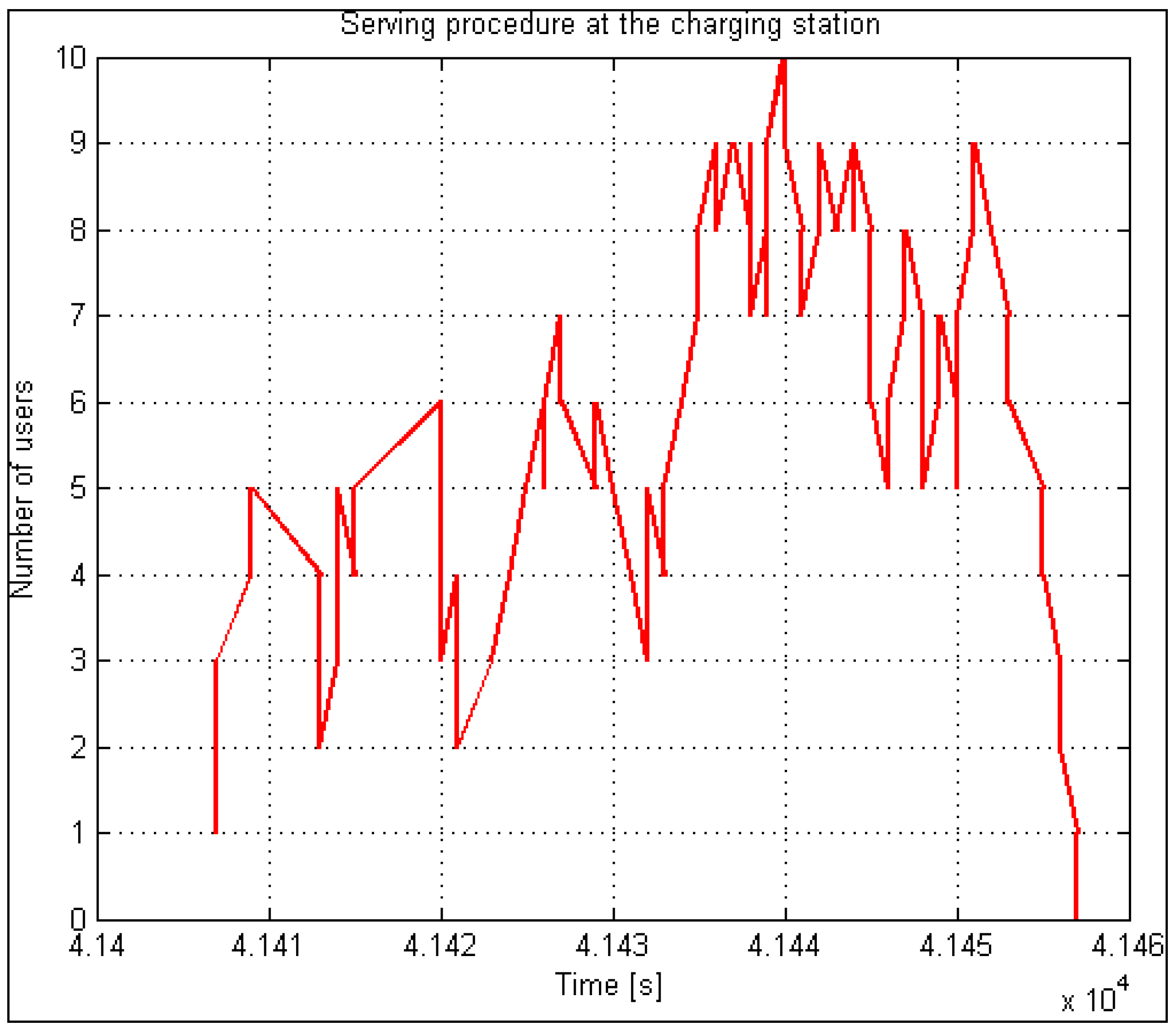
At the same time, other inputs can receive users and serve them according to the rules of the duration of the serving activity. For this purpose, we have introduced an additional parameter, Z(t), which records the number of occupied input capacities in terms of time. It functions on the principle of incrementation and decrementation. In the initial state, its value is equivalent to the value of input capacities. Suppose we have ten inputs available (Z(0) = 10). As soon as the service system receives a user, Z(t) is decreased by a decrement of 1. It keeps this value if the serving of a specific user (electric vehicle) is not finished. Every finished “vehicle-user” Z(t) is incremented by value 1. When Z(t) reaches value 0, this is a clear signal that the system cannot receive or serve new demands. The process treats users according to the system operation regime (rejecting, waiting in line). With the introduced parameter, we can examine the utilization of the system over an extended period (a day) or observe usage during peak times. The temporary value of the indicator Z(t) represents the provisional number of free input capacities.

Every input is also indexed. Different charging durations introduce indexation. The ability to determine the currently accessible inputs influences the freeing of input capacities. By doing so, we can load available inputs even when some in-between inputs are already occupied.

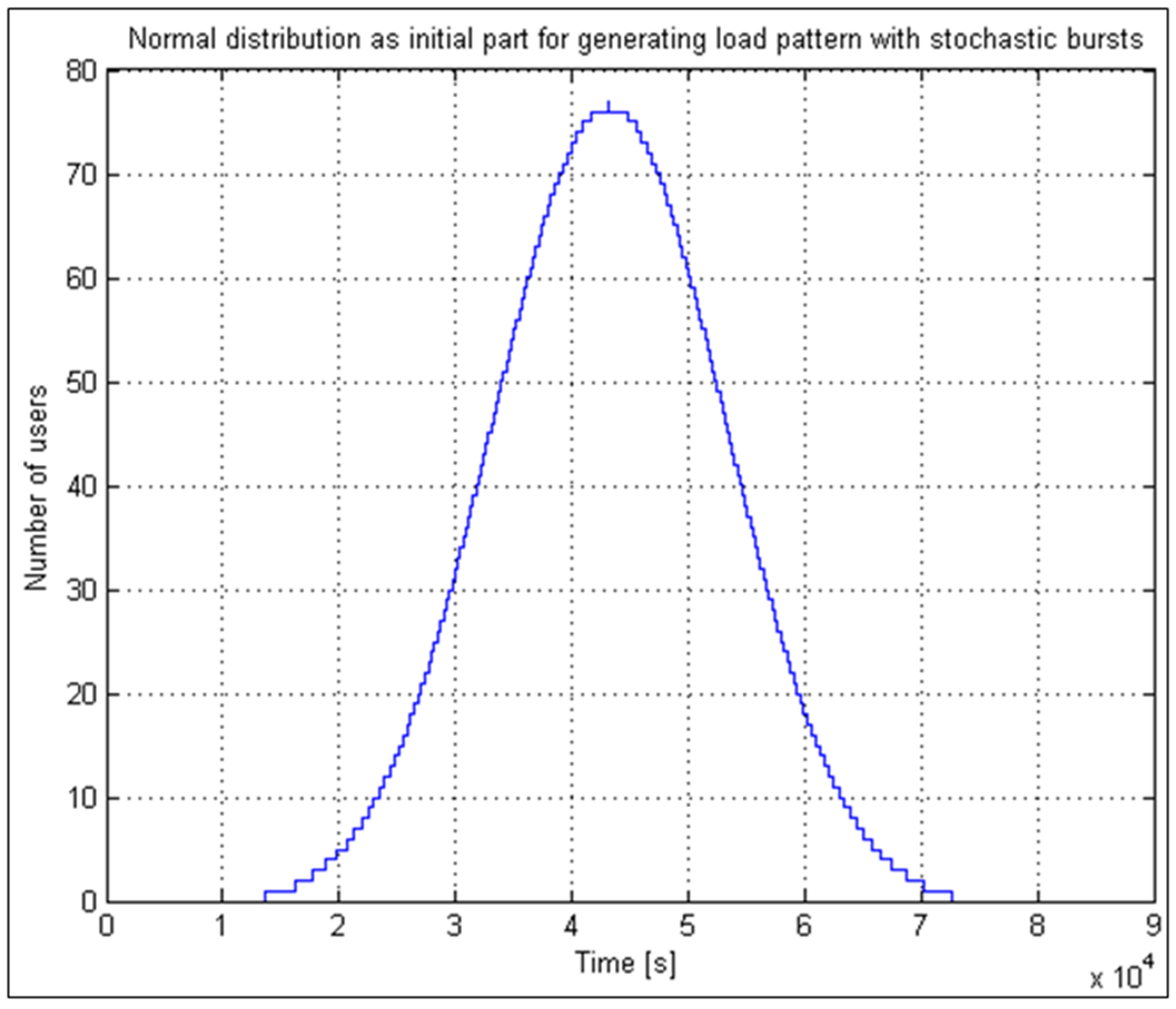
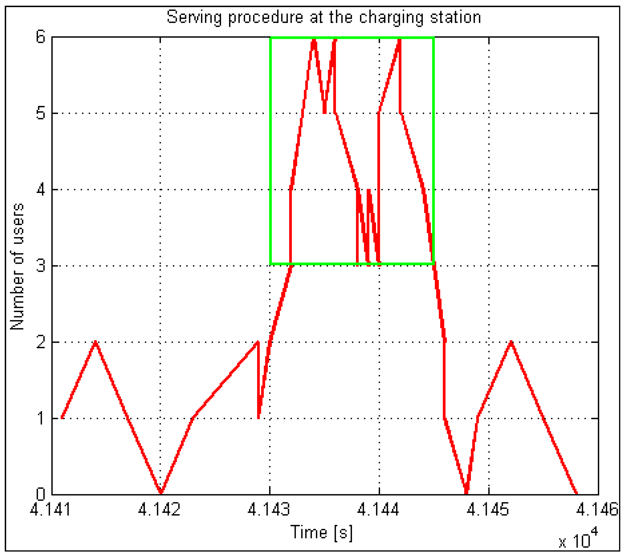
2.2. Peak-Load Model

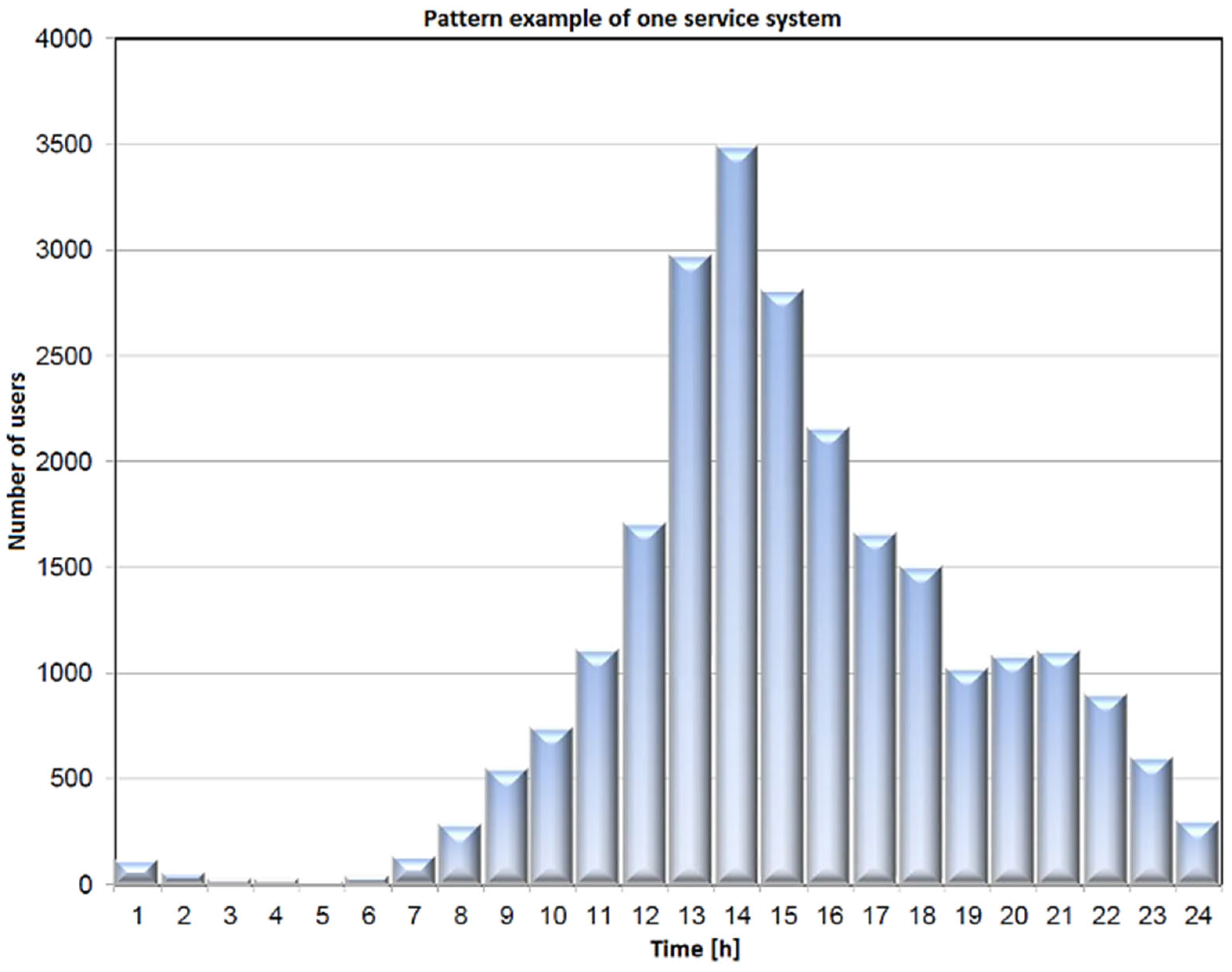
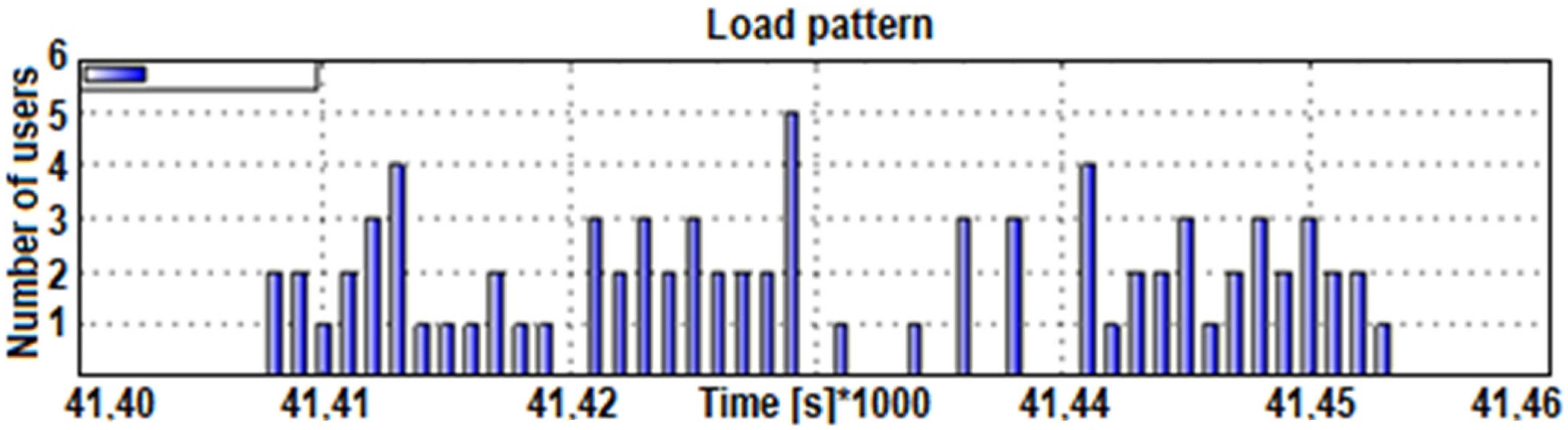
In an analysis of the performance of the EV charging system, the histogram of the number of bursts of demands followed a Gaussian probability density function and showed that, out of all bursts during one day, only one was dominant. Approximately 70 percent of everyday demands come from it. There is a burst of approximately one hour duration in this period, so we call it “peak” or “rush hour”. The charging system simulator implements this model separately in a thread. It can start performing at any point of the probability density function and runs continuously.

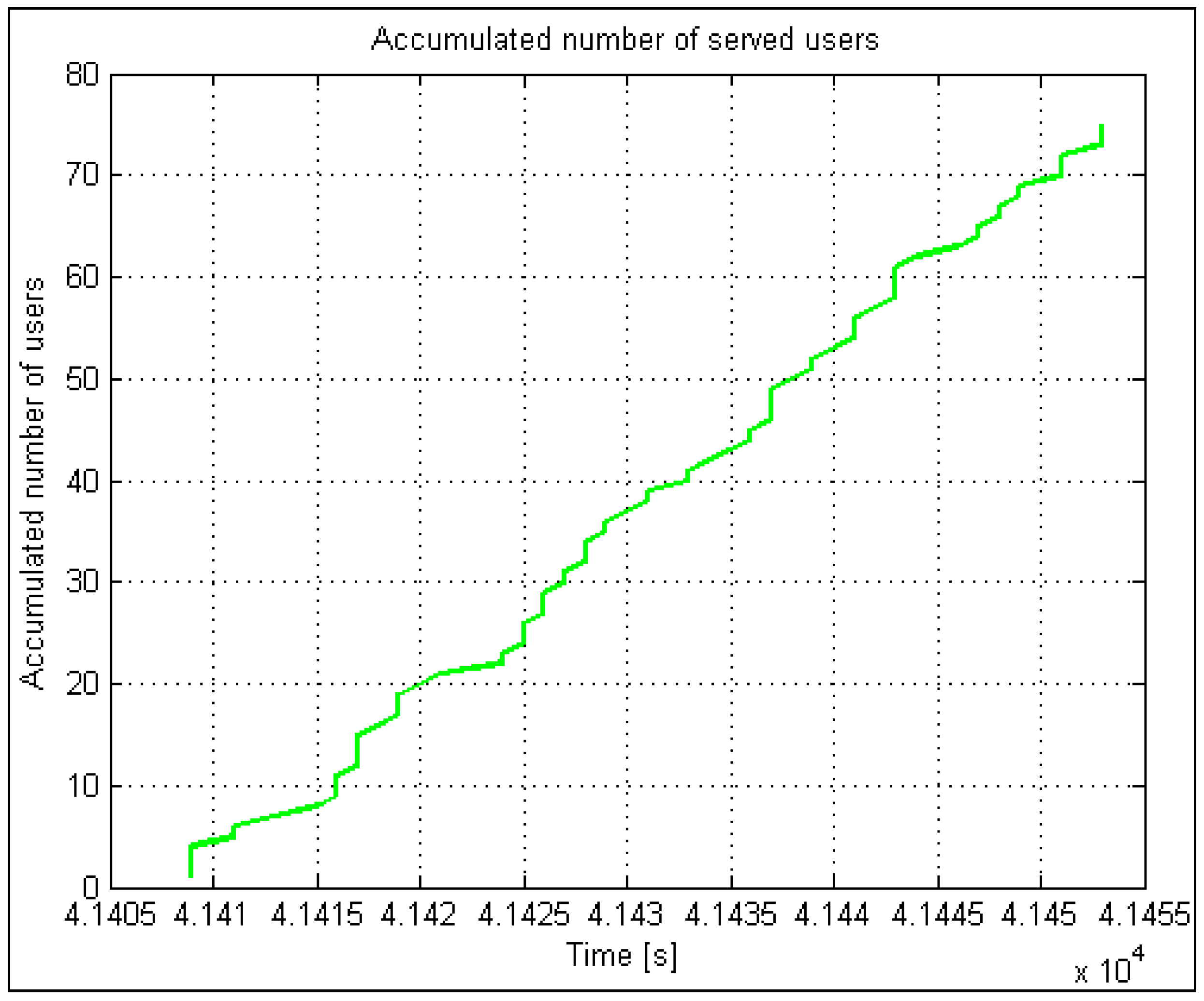
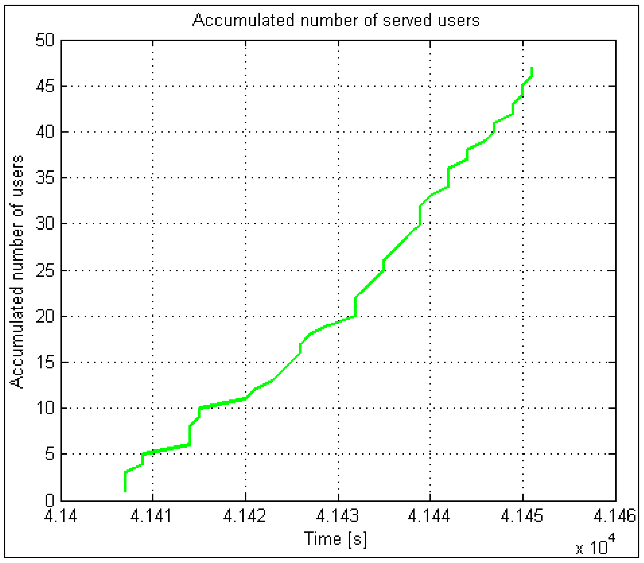
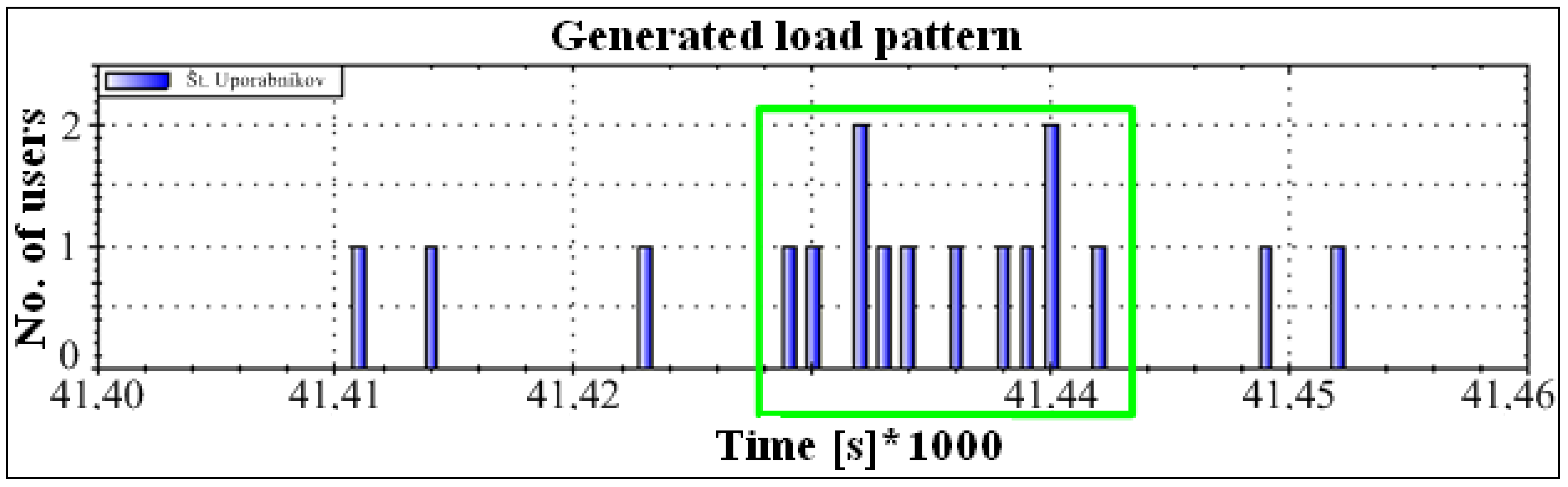
Figure 2 illustrates an example of rush-hour traffic. It is evident from the figure that almost 3500 users appear within one hour.

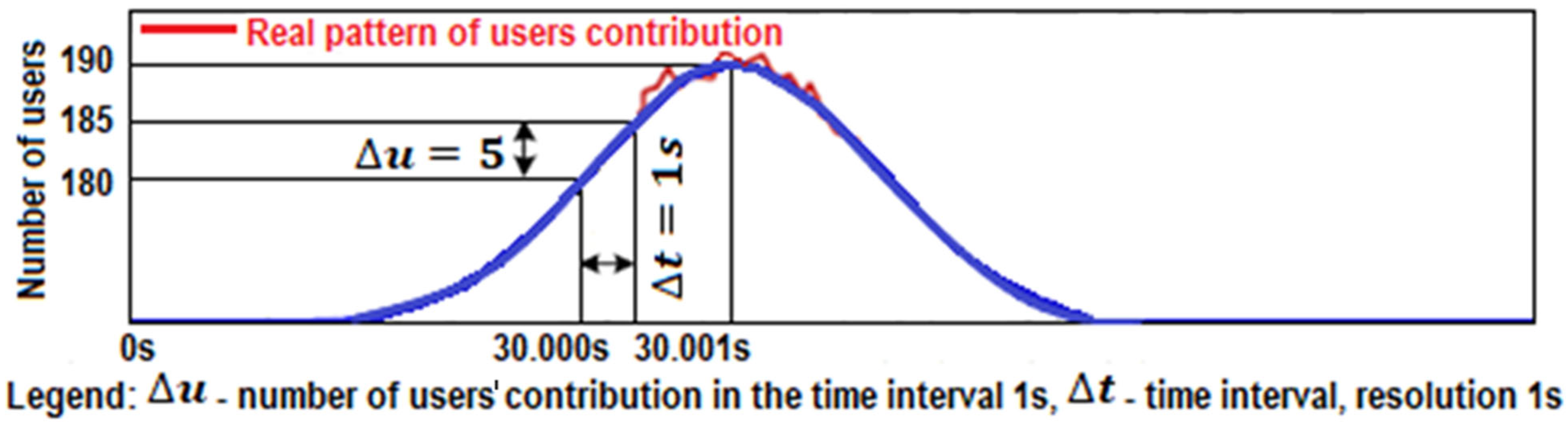
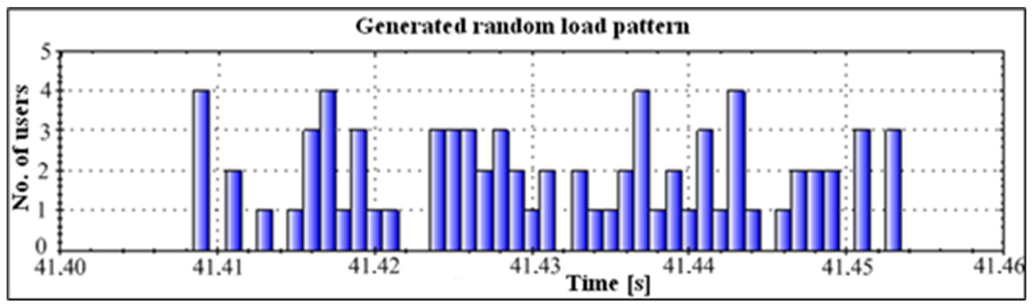
We can determine the normal distribution parameters because we know the number of users within the peak load (statistical analysis) and the duration of such an interval (Figure 2). According to the increment (left increasing tail), the proposed method generates for users (increment) the times of triggering visits within the interval using pseudo-randomness, which already at the beginning of implementation ensures a random pattern within statistical limits. We can hypothetically (according to Figure 3) assume to have 200 demands (scooters, users, calls, transactions) within a 15-min interval. Using the statistical data and the previously described procedures, we design a pattern with a reference normal distribution of users increment (left tail—see Figure 3). The proposed method seeks a solution that satisfies a wide range of load patterns and set criteria. The criteria are set to consider the worst-case scenario results in terms of waiting time, allowable waiting period threshold, and allowed rejection threshold. All load patterns are created from the same statistics. All the listed criteria are considered with the included automatic analysis in the optimization loop, presented in Section 2.5. It looks for a near-optimal (the expression “near” is used for a reason, as in practice it is very difficult to repeat a pattern that is identical to the previous. Because the method generates a certain number of patterns, the acquired solution is highly probably accurate, but there is still a chance of an untested pattern, for which this is not true. That is why we use the expression “near-optimal”) solution in a manner that is shown in Figure 4.

The parameters for the peak-load model, which is also based on a normal distribution function, were calculated using many peak-hour patterns managed by the EasyFit tool [43]. We followed the same approach for the peak-load model as we did for the model for real and lammer users.

2.3. Description of the Algorithm for Triggering EV Charging Event

Data on users, their number, duration, and the charging starts, determined based on previously described and defined methods, are saved in the dynamic data structure. Because the whole method is time-continuous oriented, the demand triggering model is accordingly adjusted. A transaction or call is triggered based on the system time, considering the triggering function’s criteria. A specific thread is used to carry out the triggering operation. The function continuously searches the dynamic data structure. New users are added according to the movement on the normal distribution curve for “peak hour” (Figure 3) and look for users whose triggering time coincides with the system time. A minimum delay in the range of 10 ms is allowed for searching an extensive data structure with millions of users. We compare the participant’s specific time with temporary real system time during this process. If there is a match, the demand is triggered (on the condition that the user has not been accepted yet, is still active, etc.). In the second step, the function checks whether the abovementioned indicator of available capacities Z(t) has a value different from 0. If the answer is positive, the demand is accepted. Suppose not the usual match is treated according to the chosen operation regime (rejection, repeated attempt, or a queue—regimes supported by the proposed method). An accepted demand in the service system takes up the input as long as the completion function does not fulfill the completion criterion. A separate thread performs the completion function with a limited time delay of 1 ms. At the same time, this value represents the lower limit in scaling the parameters for the need to speed up the simulation. In response to the time running out for active demands (flag indicates whether they have been accepted into the system), a thread iteratively searches the dynamic data structure using the temporary system time. Because every user in the dynamic data structure has a defined time of the “transaction” and its duration (see subsection on random assignment of time of demand/charging within the observed interval), the completion is the sum of the start and the duration. From this perspective, we have available all the data necessary for operation. When the thread with the performed criteria completion function determines that the demand ran out, it deletes the accepted flag and puts a completed flag. Suppose the option for reassignment of data to a user, etc., is chosen with the method. According to the procedures mentioned above, the user receives new parameters at the beginning and throughout the duration. Therefore, the user can determine when to “visit” the system again. In this case, the service system’s communication and loading procedures disregard the user. With the release of the EV charge, Z(t) increases. We want the model to reflect actual user behavior. For example, if a user does not receive the service, there is a high probability that they will try again. The method can consider these factors in user choice (integrated and implemented). During the simulation, statistical data are collected by accepting, terminating, and rejecting users. Therefore, statistical information is continuously updated on the simulation/emulation tool [44].

2.4. Applied and Implemented Optimization Methods

Because, in our case, we are generating pseudorandom load patterns with stochastic characteristics within a deterministically defined observation interval, optimization belongs to the area of stochastic programming. For optimization, we first used the method of incrementation/decrementation of the service capacity parameter in terms of the allowed threshold or criterion of rejected users. Because the used method has certain deficiencies (very time-consuming—see paper [44] about looking for a solution), we provided two different processes to speed up the search for an optimal solution. These are:

• tangent method and
• the secant method.

In our case, the tangent method has been ineffective since it requires knowing the derivative at a specific point of the criteria function, which is quite time-consuming. We proceeded with the secant method. With it, we avoid finding the derivatives of the criterion function in specific points. For this purpose, we substitute the derivative of a specific point with an assessment, written down as a differential quotient (5):

$$f^{\prime }\left(\frac{f\left(a_n\right)-f\left(a_{n-1}\right)}{a_n-a_{n-1}}\right)$$

(5)

To assess the next element, an approximation in the secant method, we use the following iteration Expression (6):

$$a_{n+1}=a_n-\frac{a_n-a_{n-1}}{f\left(a_n\right)-f\left(a_{n-1}\right)}·f\left(a_n\right)$$

(6)

Considering the representation in the Cartesian diagram, the difference ($a_n-a_{n-1}$) represents the interval on the abscissa marked as (Δa). The difference of functions [f(a_n) − f(a_n−1)] for the chosen points represents the interval on the ordinate marked as (Δy). Considering the previous equation and the relevant connections, it can be expressed as in Equation (7).

$$a_{n+1}=a_n-\frac{\Delta a}{\Delta y}·f\left(a_n\right)$$

(7)

The difference $\frac{\Delta a}{\Delta y}$ is then converted into factor A, which depends on the temporary point a. The final equation for calculating a new approximation takes the following form:

$$a_{n+1}=a_n-A_n·f\left(a_n\right)$$

(8)

When carrying out the secant method, we need an initial interval, defined by points $a_0$ and $a_1$. These are the initial conditions for calculating the successive approximation of the secant method. With every following calculation of an approximation, we are closer to a solution, which leads us under the threshold of allowed rejected demands. Optimization is often performed with this method because it is fast and straightforward (but not as good as the tangent method). There is no need to find the derivative. Still, based on simple iteration, we find the optimal solution, which is lower than the allowable deviation on the condition of two consecutive steps (see the figure below).

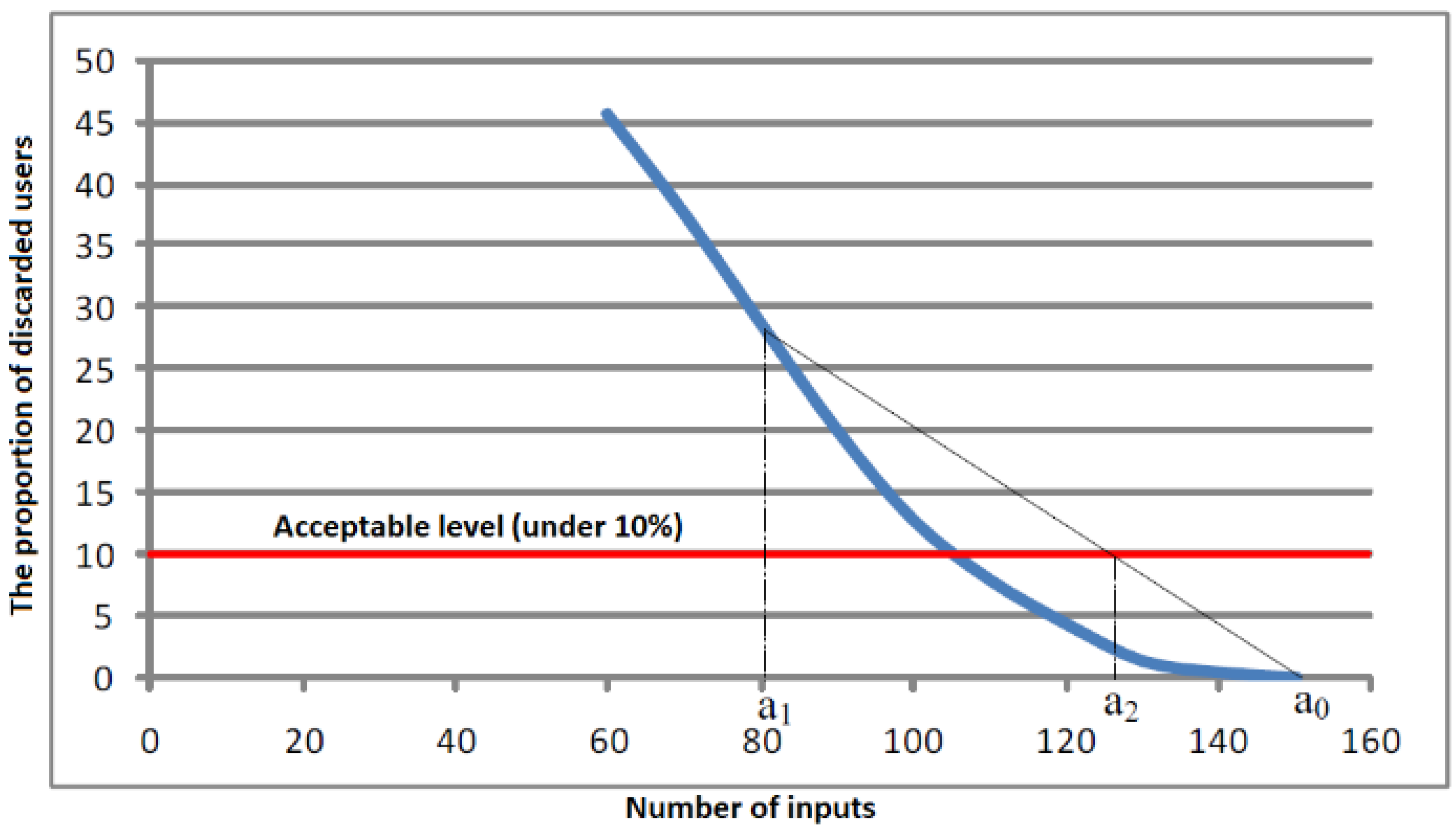
Figure 5 shows a real example of a criterion function. A short experiment shows that convergence speed depends on the initial conditions (interval selection). For the threshold of 10% (Figure 5), we quickly obtain a not necessarily optimal solution. One can find the optimal solution by further bisection of the interval, but the incrementation method mentioned here serves this purpose better [44]. From this perspective, we find an approximation with a secant method. In the second step, with the combined incrementation/decrementation method, we see the optimal solution with a high degree of repeatability on different load patterns resulting from the same statistical distribution.

Our second step is to find a better solution in the vicinity of the approximate solution using the incremental method. When looking for an improved solution, we consider the repeatability and coverage of a wide range of stochastic load patterns based on the same statistical distribution. When looking for a solution with the secant method, we limit or round up the approximations to integer values because we are looking for the optimal number of service capacities (lines, service places, etc.), which can be described only with the set of positive integers ${\mathbb{Z}}^{+}$.

2.5. Automatic Analysis as a Feedback Loop in the Optimization Process

For previously described and used optimization techniques based on incrementing or decrementing the service capacity parameter, we also introduced an automatic analysis of simulation results and individual factors as indicators of possible problems in the service system. The introduced factors, presented in detail below, are auxiliary elements in the optimization process.

Every time a thriving demand is accepted or rejected, the algorithm records a time code. The proportionality observation R(t) is another factor created using a specific scenario’s collected data. Each sample value calculates the proportionality factor R(t), resulting in the characteristic R(t).

$$R\left(t\right)=\frac{\mathit{No}\mathit{of}{\mathit{Users}}_{\left(t\right)}}{\mathit{No}\mathit{of}{\mathit{Inputs}}_{\left(t\right)}}$$

(9)

The time index t represents the sampling time. When R(t) is much smaller than 1, the service system’s predicted number of input capacities is sufficient. Whenever the factor approaches 0.7, there is a high probability that the system will reject requests as it will be overloaded. Calculated concurrently, that is, during the simulation, the factor R(t) provides a good indicator that alerts us to any unwanted events occurring in the system. An important purpose of the factor R(t) is to determine when and where it is rational to increase input capacity (the demand for dynamic relocation of service capacities).

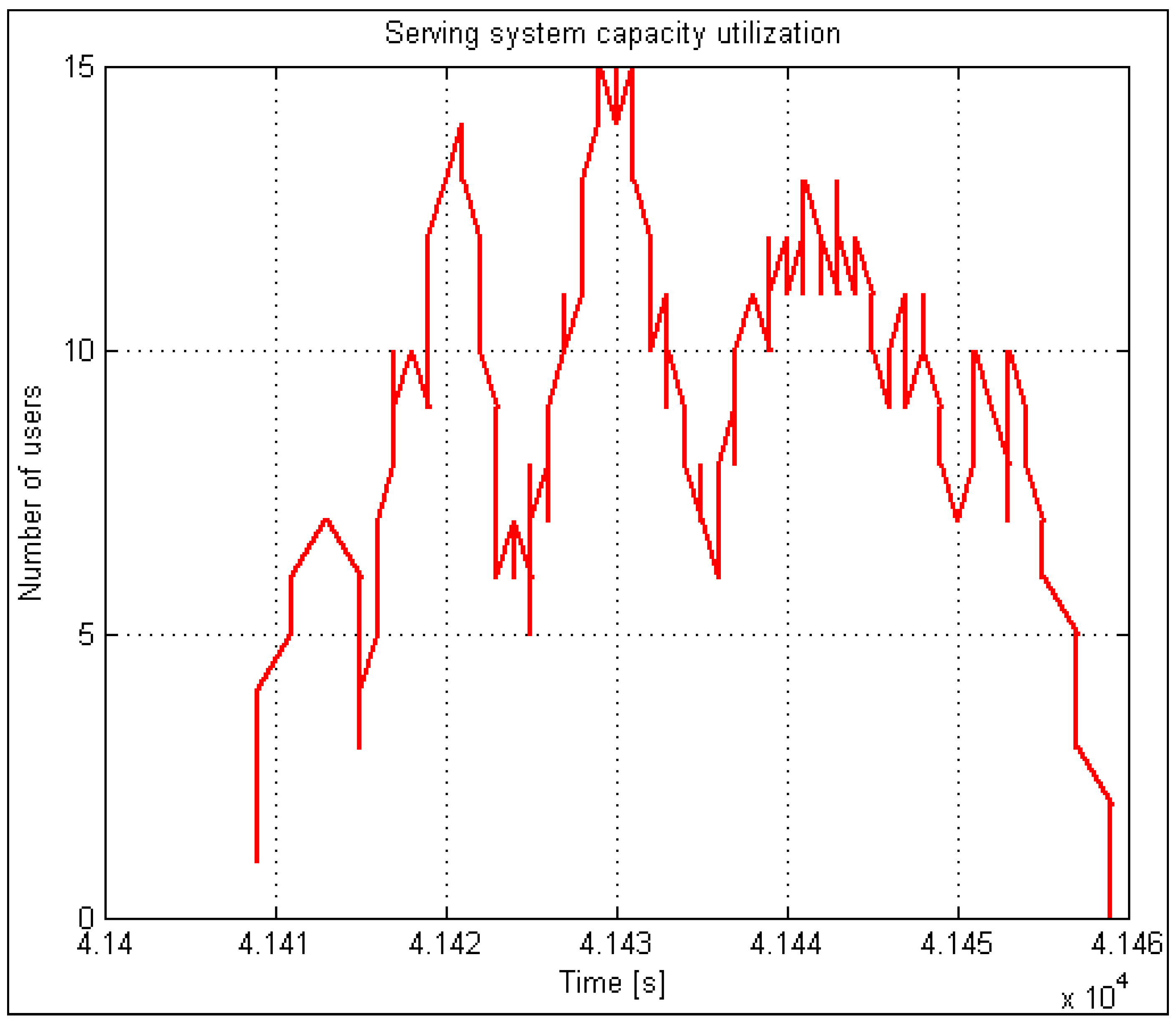
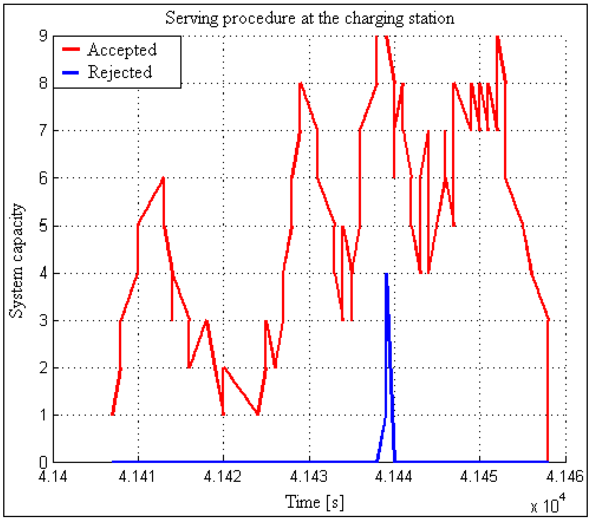
During the simulation, automatic data collection on the rejected and accepted requests for each time tag is also crucial for optimization (Figure 6). This factor or relation is marked as K(t) and called the calculated relation acceptance/rejection curve. Depending on the time, it points out the problematic areas. With Equation (10), we calculate the factor K(t).

$$K\left(t\right)=\frac{\mathit{Rejected}{\mathit{Requests}}_{\left(t\right)}}{\mathit{Accepted}{\mathit{Requests}}_{\left(t\right)}}$$

(10)

Regarding time, K(t) is a curve on the lower side limited with 0 and practically unlimited upwards or limited with the relation between the maximum number of all users and the maximum number of available service capacities. The values and the meaning of the obtained curve K(t) are the following: 0 at a particular time index indicates that no input demand has been rejected (capacity is still available, but it is not fully utilized). Otherwise, when factor K at a given time index t has a value different from 0, this means that in this area, rejection of demands happened (when considering the queue in an x-system, factors K and R, and functions K(t) and R(t) are irrelevant and are not considered). In the case of planning and service capacity optimization for systems with queues, function W(t) applies, describing the changing of the queue subject to time. Function W(t) combines the permeability and queuing factors in the optimization process. In this process, the functions R(t) together with K(t) and W(t) are mutually exclusive and depend on the type of the considered service system (with or without a queue). All three presented functions represent automatic indicators of the successful operation of a specific (considered) service system.

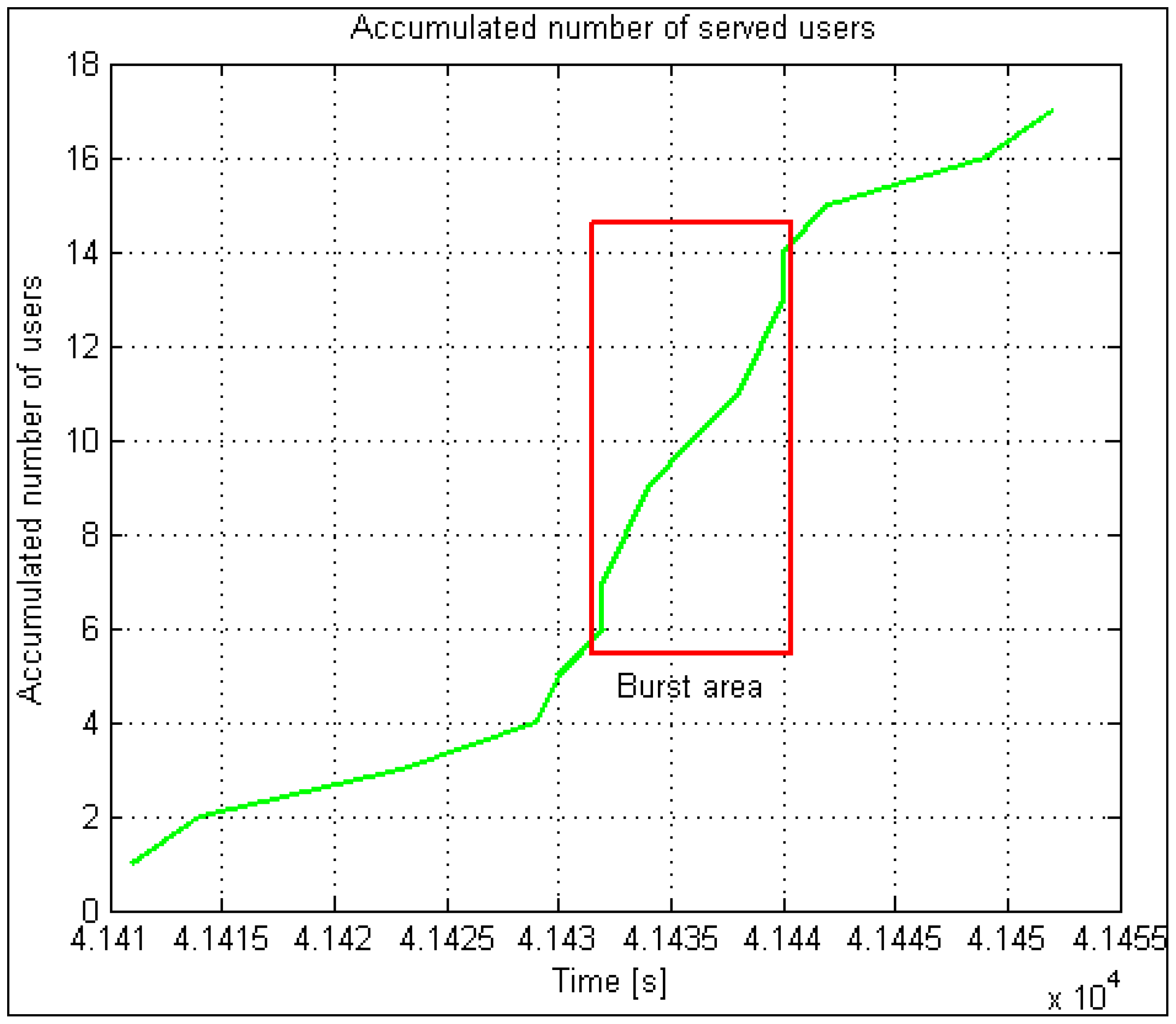
The accumulated number of accepted and rejected users and the number of lammer users are vital statistics in automatic results. Calculating the statistical percentage is easy with a balance and a percentage calculation on the accumulative number of lammer users. The same applies to the accumulated number of accepted and rejected users. These data serve for model validation compared to the data acquired from a real system. All the presented parameters significantly simplify and speed up the analysis process and, consequently, the optimization process when searching for a “near” optimal solution.

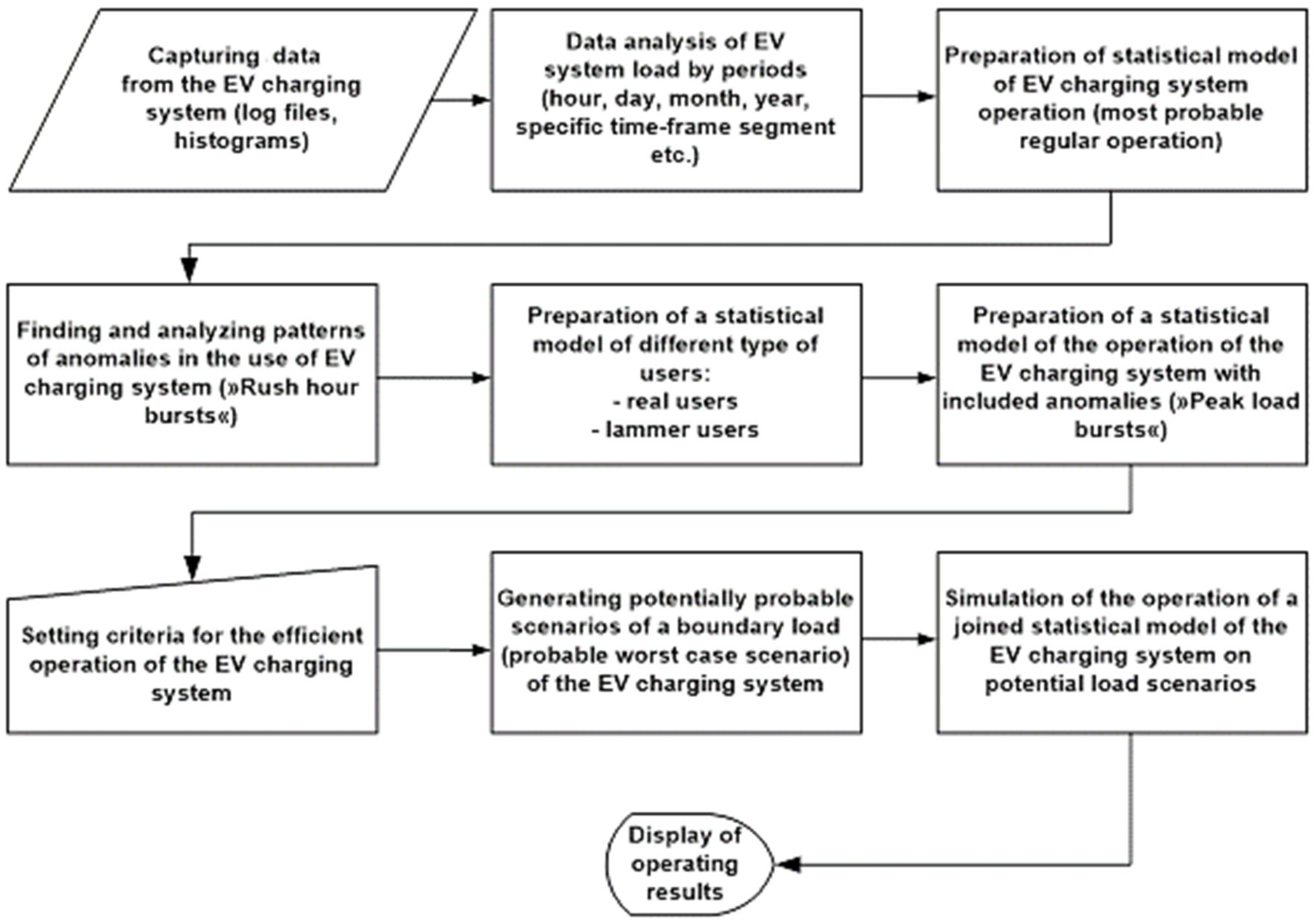
2.6. Designing the Proposed Method

Figure 7 illustrates the phases of implementation and operation of the proposed method. Automatic analysis is a guideline in terms of time demandingness and complexity. On the other hand, it also serves as a simultaneous link in the feedback connection and optimization process. We look for the necessary number of service places, lines, etc. Trends in software development, methods, simulation tools, etc., are pointing towards a high degree of automatization so that the user or operator is minimally burdened. However, a certain degree of knowledge about the considered area and the accompanying topics is necessary even in these situations. When designing the method described above, we thus focused on minimizing the requirements for such knowledge. The operator obtains the necessary statistics from actual measurements but can also generate them empirically. At the beginning of the simulation, the operator enters the required statistical data. In addition, the operator must decide what type of system to use, i.e., whether users (so-called “transactions”) are repeated or not, whether a queue is included or not, and how users (e.g., transactions) are scheduled during peak load periods. The rest of the analysis is one of the inputs in the optimization process, and an advanced tool automatically performs the optimization. No intermediary intervention is required from the operator to find a near-optimal solution. The operator also has available an empirical regime meant to test what-if scenarios. The operator intervenes with a change of statistical input data and observes what happens in the system. The emulation mode is the third regime in which the developed tool with the implemented method can function. In other words, statistical data (transaction lengths, their arrangement, duration, etc.) are read from the “.log” file, which substitutes the segment of the proposed method model where users, transactions, etc., are modeled and generated. In this mode, the user is only interested in how the system behaves in certain moments. With emulation, the proposed method can optimize capacity by optimizing the performance of the services. However, it is more sensible to analyze patterns in a longer time frame and choose from this range of worst-case scenarios, based on which the system is optimized.

An average pattern is used to optimize the existing system through emulation and optimization if no patterns stand out. Its multipurpose nature makes the proposed method and implementation appropriate.

3. Qualitative Discussion

The author in [32] proposes a simulation model that uses a deterministic approach to perform an analysis whose result is the necessary capacity of charging stations for electric scooters considering random needs and factors. This concept contrasts with ours, where the occurrence of events is deterministic to a certain extent (the assumed number of events can be estimated sufficiently well in the “rush hour”). Still, their occurrence and the formation of patterns are entirely stochastic. Predicting the “rush hour” periods is also a part of the deterministic segment, as we were able to precisely assess when these periods occur for the Margento service system [44] (analysis of statistical data). For this reason, the proposed method has only the interval of maximum service system load determined deterministically.

In contrast, considering the normal distribution, transaction increment, and pseudorandom assignment of transaction triggering time, the load pattern reflects stochastic characteristics. In other words, this means that transaction occurrence is completely stochastic within a deterministically determined interval, which introduces bursts. The latter need special treatment and can cause long queues and overloads in certain moments in slow systems (poor dynamics), where the discussed charging stations also belong. The author, in his work, does not consider stochastics or potential stochastic bursts but consistently follows the increments of normal distribution in the observed period (from 8:00 h till 18:00 h). Because it is difficult to find the ideal normal distribution in the “rush hour” period on such a charging station, the author, in this case, “smoothed out” all the peaks (bursts) and approximated them with the classic normal distribution. Each such approximation or linearization leads to an inaccurate or only approximate result. We adopted a completely different approach, as normal distribution in generating a stochastic “rush hour” pattern is only basic information on the number of transactions and their increment during a continuous observation. We thus do not delete the bursts but instead recreate them. Since we use a “pseudorandom” thread, we can generate n patterns from the same statistical data. We can find the optimal solution for either the so-called “worst-case” scenario or a solution based on x tested patterns generated from the same seed (same primary statistical data, same length of observation, same normal distribution, etc.). In the case of known input load statistics, the proposed method can work completely deterministically (predictably). We can recreate the load pattern using emulations and automatic analysis of log files.

In the model [32], the author supposes he knows the loads of individual charging station locations, the number of active/functioning charging places, the time component of battery charging, and bottlenecks (primary data for the proposed method). By using statistical functions based on measured data, the author in [32] models individual charging stations’ service.The author thus largely depends on the statistics of the average utilization of charging stations. This statistic is, for him, an indicator for the potential relocation of charging stations (relocation in terms of geographic position—irrelevant for us) or an indicator for increasing the number of charging places (our area). Considering the parameter of average utilization is, from our perspective, somewhat risky, as a single burst in the service system with a slow dynamic (which a charging station is) can cause long queues. This method can also solve the problem of relating the number of service places with the waiting time or rejection.

If we compare the two methods again, we do not consider it wise to rely on average utilization, which we have already shown and confirmed in [44] (see the second experimental scenario). In this area, the stochastic burst has too much influence on the accuracy and suitability of the final result.

The author used linearization to design and model his solution. He used this method to solve the problem of the number of kilometers covered and the time of charging (depending on how empty the electric scooter battery is). Such an approach contradicts our idea, as we do not introduce simplifications. Still, we consider the situation as it is or might be in the future (prediction ability).

Based on those mentioned above, one single station can be, in terms of behavior, treated the same as the service system presented in [44]. As a result, we can use the proposed method to plan and optimize the number of charging places at the consideration charging station (see next section). It is possible to translate the model of users, transactions, and calls from the system [44] into the model of electric scooters in the observation interval. Changing the parameters of the normal distribution function of the relevant model allows us to convert the transaction model into the model of the charging duration. It includes a broad spectrum of users (empty batteries, partially empty batteries, nearly full batteries, etc.). The author does not consider the factor of batteries with a failure, which often appears in practice, especially in the high intensity of charging. Still, it can be regarded as the proposed method, including a model of lammer users (transactions, calls). The latter can be analogically translated into the model of charging duration for batteries with a failure, again with a modification of normal distribution, which in our method and consequently also in the simulation/emulation model is used to describe lammer callers.

Like us, the author divided the problem into several more minor issues, where he systematically modeled each segment individually. In this respect, we are equivalent. In the proposed method, we consider individual segments (charging duration, partially full batteries, the percentage of batteries with a failure, etc.) separately with submodels within the entirety. In statistical data processing, the author concluded that a normal distribution could describe the average speed of electric scooters. They came to the same conclusion when describing the stops at individual tourist points. From our point of view, these data are irrelevant because we do not plan the geographical positioning of charging stations but use the method of precise planning and optimization of charging points. For this reason, the included feedback automatic optimization loop with an optimization method, automated result analysis, etc., is vital for the proposed method and represents an additional difference between the methods. In these terms, we rely on the statistical data in the observation interval [32] and the data on charging duration and data on battery emptiness which the author determined with the mentioned normal distributions (average speed, stops, etc., factors that influence the final condition of the battery in every electric vehicle). The state of the batteries at charging stations is the starting point for directly comparing our proposed and reference methods.

4. Experiments and Simulation Results of Both Methods

We have included the statistical data given by the author in his paper [32] (see the table below) in our proposed method. Since the author did not explicitly provide the mean value of the charging time, we statistically determined this parameter using the available data. In the same way, we determined the percentage of electric vehicles with battery failure. However, it significantly affects the charging process’s dynamics and the charging slots’ occupancy. Three scenarios were run in an experiment with varying charging station capacities (chargers) and EV numbers (users) as shown in

Table 1. Service volume and performance for the allocation of recharging stations (Author’s paper, ([32], p. 5)).

Service Volume and Performance for the Allocation of Recharging Stations (15,1,14,15,15,15)
Site	Electric Scooter Market Share (%)	Number of Recharging Stations	Electric Scooter Volume	Average Waiting Time (s)	Average Length of Weight (no./s)	Average Utilization
Citou aquarium	50	15	75	0	0	56.2
	30	15	47	0	0	33.4
	10	15	17	0	0	15.8

. Note: For a better comparison of our results with the author’s, the comparison refers to the author’s paper ([32], p. 5), namely all three examples after the line Citou aquarium:

4.1. Experiment 1. The Number of Charging Places P = 15, the Number of Users = 75

Table 2. Coefficients of polynomials P and Q are used to obtain the normal distribution values.

Parameter	Normal Value	Scaled Value
Observation time	8.00 h—18.00 h (36,000 s)	36 s
Service capacity	15	15
Number of users in the observed interval	75	75
Mean value of the charging time (N)	6500 s	6.5 s
Standard deviation (N)	400 s	0.4 s
Mean value of the charging time for a scooter with a battery failure (O)	1000 s	1 s
Standard deviation (O)	200 s	0.2 s
Percentage of scooters with a battery failure	1.35%	1.35%
Allowed percentage of rejected users (%)	0%	0%
Allowed waiting time in the queue (s)	0 s	0 s

shows the proposed method’s parameters for predicting the events in the service system with 15 service places and 75 users between 8:00 h and 18:00 h. Scaled values, shown in the far-right column, speed up the simulation, as the method uses the so-called continuous-time simulation model. According to the scaled value of the observed interval, other parameters are accordingly scaled, such as the mean value of charging time for batteries with no failure signs (N), standard deviation (N), a mean value of charging time for batteries with a failure (O), standard deviation (O), etc. The mean value of charging time for batteries with failure is relatively low because modern charging equipment, including diagnostic tools, identifies battery failure in a short period. A user such as this is generally removed from the charging place, so the charging place becomes free, which changes the dynamics. Because such an EV goes to a workshop to change the battery with a new full one, and because the percentage of such batteries can be even higher in one day as predicted, this element is essential in terms of permeability in the “peak load” intervals. The paper [32] does not mention this factor. Still, we have already included it, as it is one of the accuracy conditions and, consequently, a condition of accurate planning. We have generated random charging system load patterns with the normal distribution (Figure 8) and observation interval. Figure 9 shows one of the patterns.

Based on the analysis of obtained solutions and considering random patterns (in our case, we performed the analysis on twenty patterns), we found the average utilization as the only factor for direct comparison with the author’s results. A set of random patterns was generated from the data in Table 1. When generating patterns, we used only the left increasing tail of a normal distribution, where the number of users is increasing (the right, decreasing tail is not interesting for us).

We talk of bursts in the simulation when many users appear in the service system simultaneously or approximately at the same time (they are not equally distributed). Figure 9 shows burst moments, where two, three, or even four users appeared in the system simultaneously (peaks).

The simulated service system with a capacity of 15 service lines responded to a generated pattern from Figure 9 with the activity shown in Figure 10. The latter can calculate the average utilization during the whole observation period. Although we avoid such parameters and assessments in our method as much as possible, we made an exception in this case. The reference method [32] does not present a load or utilization curve concerning time, so we introduced an exception. For this purpose, the parameter of average utilization is the only parameter we can validate in the proposed method compared to the reference one, as the author gives an average utilization as the result of his model.

The result of the service system utilization (Figure 10) shows that the average utilization is slightly over 50%. The problem which we have been emphasizing throughout the paper is stochastic bursts. One of them can be seen in Figure 10, where the system is full at its peak. Although the average utilization is relatively low, a few added users could completely change the picture. Waiting and long queues would appear, which we want to avoid with the proposed method and predictions. For generating different random patterns, we have used the same statistical data. All patterns produced similar results. In Figure 11, we can see how the EV charging system served users for a given experiment over the observed period.

However, bursts were amplitude-wise differently arranged and localized for the number of users (75) and the service capacity (15).

The simulation results show that all users were served without waiting (Figure 10). With the same parameters (the observed interval, distributions, etc.), an additional two users could hypothetically influence a concentration in the load pattern, which would cause queues. In this case, we can use prediction and change, concentration, and dispersal of the load pattern to look for optimal solutions for the operator, us, and the end-user (looking for compromises). A direct comparison of the proposed method’s results with the author’s results [32] is shown in the table below (

Table 3. A comparison of the average utilization of the service system for our method and reference method.

Method	Number of Service Places	Number of Users	Average Utilization [%]
Proposed	15	75	60.4
Reference	15	75	56.2

):

A direct comparison shows a difference of 4.2 percent in the average utilization between both methods—the difference results from the empirical determination of charging time. As a result of these findings, we can emphasize the importance of stochastic bursts within a deterministically determined observation interval. We should also again mention the reliance on a misleading value of average utilization of service capacities. One might think that more than 30% of available capacities are still free. While this is true, we cannot expect uniform distribution from such systems. The subject of our investigation should be peaks, overloads, and bursts. When peaks appear can be deterministically determined based on statistical data, but how “elements” are arranged within peaks or a peak (in case of a normal distribution) and how bursts occur is entirely random. For this reason, one should not expect repeatable burst patterns in this segment of discussed systems. A specific difference is also attributable to our random pattern being different from paper [32].

4.2. Experiment 2. The Number of Charging Places P = 15, the Number of Users = 47

In the second experiment, we kept the parameters from Table 2. We only decreased the number of users from 75 to 47 in the same observation period (Figure 12 presents the load pattern of 47 users). During the simulation, we again monitored the average utilization of the service system, which was a basis for direct comparison with the author’s approach [32].

Figure 13 illustrates the utilization of the system and its response to a random load pattern. The random pattern is concentrated in several places, meaning the burst is reasonably uniform within the observed interval. Considering the concentration of users in the last third, we can suppose that the service system load will increase in that part. In Figure 13, we see the consequence of load concentration or burst. Because in this example the number of users is almost halved compared to the previous one, the average system load is lower. The average utilization is 38.23%.

With this experiment, the maximum system load does not exceed ten charging places, which means that such a charging station is over-dimensioned for a predicted number of users. We also tested different sets of input patterns for the same parameters but did not exceed the limit from Figure 13 in any of the tests.

A direct comparison of the results of both methods shows a difference of 4.83% (

Table 4. A comparison of the average utilization of the service system for our method and the author’s method.

Method	Number of Service Places	Number of Users	Average Utilization [%]
Proposed	15	47	38.23
Reference	15	47	33.4

). The reasons for this difference are the same as in the previous experiment.

We can accurately assess the redundancy needed in the worst-case scenario by generating several consecutive patterns on the same data. The average utilization of 35% represented the mean value, with the deviation always being in the range of ±4%. By using prediction and pattern searching, including the “worst-case” scenario, we can confidently claim that with the service capacity P = 12, users will not have to wait for a free charging place, and no user will be rejected. Excluding the “worst case” scenario, ten lines can suffice for the system with the same criteria. By considering the allowed waiting for time threshold and the permitted percentage of rejected users in the optimization method, the number of service places can be reduced for economic reasons.

We suppose the threshold for rejected users is 11% (which with 47 users means five users can be rejected). In this case, the optimization method included in the proposed method, including the “worst-case” scenario, solves nine lines, as shown in Figure 14 (again for the “worst-case”).

Figure 15 clearly shows what happens in the EV charging system when user rejections start to appear (blue line).

Average utilization is 58.64% if we consider the 11% threshold. Furthermore, it shows that average utilization is not credible; instead, the relationship between the percentage of rejected users and the percentage of accepted users should be used. An increasing factor indicates problems in the service system. It is possible to present the factor as a function of time.

4.3. Experiment 3. The Number of Charging Places P = 15, the Number of Users = 17

In the third experiment, we kept the parameters from Table 1 and again decreased the number of users from 47 to 17 [32]. The observation interval was the same. Normal distribution parameters used for defining charging times and describing the charging procedure for batteries with failure are also unchanged in this experiment. The share of users with a battery failure has been decreased to 0.15 percent, meaning that at least one such user can appear in the load pattern. According to the used parameters, the method generates the following load pattern:

Compared with the previous two experiments, this randomly generated load pattern and its drastic decrease in the end-user number in the observed period are infrequent. The most significant burst appears at the peak hour. In Figure 16, a green frame marks the peak hour.

Using the proposed method, we first tested the system response to the generated pattern, the set of twenty patterns, and found the result, including a “worst-case” scenario. Figure 17 shows the results. In the case of the discussed scenario, the proposed method results reveal that the capacity of six charging locations is not exceeded. Each additional test involving twenty different random patterns did not exceed the number of simultaneously occupied charging places. Therefore, planning and implementing an EV station with such a capacity for such loads (as was the case in this experiment) makes no economic sense. The example is typical of imprecise planning of service capacities, which causes irrational investments in construction and the maintenance and updating of service capacities.

As the purpose of the proposed method is the exact prediction of the service capacities, we tested this prediction on the considered system. We set the threshold at 0% for rejected users. All users must receive service without rejections or queues. We seek a solution that complies with the set criteria with considerable repeatability by increasing or decreasing the service capacity parameter and considering the allowed percentage of rejected users based on the implemented automatic optimization loop. With all the random patterns and considering all the criteria, the method suggests the capacity of seven charging places. We also considered a random load pattern concentration possibility. By this, we also incorporate the possibility of a random pattern concentration. The following figure depicts an interim example of the service system utilization with an automatic search and optimization of the service capacity number. The method, in this case, performed the initial nine iterations with a decrementation of the initial parameter from 15 to 6 service places. The obtained result automatically performed twenty more random patterns with the same capacity and initial data. The method always predicts a reserve percentage according to the number of users, which in this case was one service place. The reserve can either concentrate or disperse because of the random generation of load patterns. The mentioned reserve can cover potential concentrations. The optimal number of service capacities is thus 7 for the described scenario. If the allowed percentage of rejected users is not 0%, the number of service capacities can be reduced and optimized, depending on the sequence of random load patterns. Such an operation regime depends on the service provider, who must compromise customer satisfaction and service quality. The proposed method analyzes different load patterns while searching for the optimal exact solution, one such random pattern is shown in Figure 18.

Using this example, one could decide to use the maximum number of occupied service capacities, but that would not be the best solution. Using the maximum number of five service lines according to the above interim load pattern would create queues for the initial scenario. The queue would be even longer in case of a random pattern concentration. It is imperative to consider all the listed factors to avoid queues in the system. The proposed method of detailed planning considers all the factors. All these factors influence the accuracy of the result. The average utilization was between 17 and 20%, with 15 service places with several iterations and pattern testing. The average utilization for the proposed seven service lines was between 38 and 41% (more accurately, 40.75%), as shown in Figure 17.

Table 5. A comparison of the average utilization of the service system for our method and the author’s method.

Method	Number of Service Places	Number of Users	Average Utilization [%]
Proposed	15	47	38.23
Reference	15	47	33.4
Proposed (optimized)	7	17	40.75

summarizes the results of such an experiment. Table 5 directly compares the average utilization between the approach [32] and the proposed method for 15 service places and 17 users.

The two previous experiments have explained the reason for the difference. Figure 19 shows the accumulated number of users during the experiment period.

Figure 19 shows a burst in the accumulated-number-of-users characteristic, where the slope of the curve visibly increases in the time frame of such a moment.

4.4. Experiment 4. The Experiment Relates to the First Experiment, Where System Users Increase from 75 to 81

This experiment proves the hypothesis we stated in the first scenario. We claimed that a few additional users could significantly change the occupancy situation. As a result, waiting times persist despite a low average utilization of service capacity. Additional six users with an unchanged service capacity create a queue and thus a waiting time—maximum and average. The simulation parameters are the same as in the first experiment. Only users increased from U = 75 to U = 81. Figure 20 shows a tested charging system load pattern.

The generated pattern loads the service capacities, as shown in Figure 20. The figure includes three individual bursts (also visible in the pattern), influencing the occupancy of the service system. Because in comparison with the first experiment the number of users has increased (by six), this addition notably influences the dynamics and the permeability of the service system. Although average utilization is slightly over 76% in the observed period, the bursts significantly affect the waiting time. In other words, average utilization is not about planning in detail. A similar situation applies to simplifications, linearization, etc. Because, in this case, we have enabled a queue in the method, we can calculate the waiting time for every moment and the average waiting time based on known charging times for individual users.

Timewise, the dynamics in the system change all the time (some batteries are charging faster, some slower, some users already come with fuller batteries, etc.), as do the dynamics in the queue. The events shown in Figure 21 illustrate the onset of the burst. Figure 22 illustrates the latter and directly depends on the events in Figure 21.

When it is necessary (when the system cannot serve all users simultaneously), we insert the whole data structure of each user into the queue. We can calculate the temporary total waiting time (Figure 22) and the average waiting time with any change in the queue.

The calculated average waiting time in the scenario in this experiment is 6385.99 s, which is slightly less than the mean value of the normal distribution of charging duration. The total longest waiting time was, in this case, 6710.27 s.

Table 6. The average waiting time when the number of users is increased from 75 to 81, and the service capacity remains the same.

Method	Previous Number of Service Places	Number of Users	Average Waiting Time According to the Previous Number of Waiting Places [s]
Proposed	15	81	6200–6450 s

shows experiment results.

In addition, the results of the presented studies could be reliably repeated with multiple consecutive iterations where the deviations remained within the ranges. We used the proposed method to find an optimal solution, as in the previous scenario. The evaluation function to increase (in this case) or decrease service capacity was also performed automatically. The iterations were performed by parameterizing either the allowed threshold (0%) or the waiting time (0 s) until they met one of the criteria. Furthermore, the scenario was iteratively repeated with the parameters from the first step, each time with a newly generated load pattern in the optimization loop. In other words, the method looked to repeat the same service capacity resulting in multiple patterns in the second step. Considering the possibility of concentration of a random pattern, the method again predicts a percentage reserve. One iteration is achieved in less than one minute using a continuous simulation technique with values scaled by 1000. Due to continuous simulation, the method finds a solution within a relatively short period (approximately 10 min). It is more than a discrete simulation method, which is irrelevant given the chosen strategy. If the method encounters a non-repeatable result during optimization, it repeatedly corrects the service capacity parameter and performs the mentioned procedure. The method repeats this step until no further corrections are necessary to ensure repeatability. In this way, there is a high probability of finding an optimal solution for a wide range of input patterns generated based on the initial statistical parameters (Table 2), which are not changed during the iterations (except for the input capacity parameter, if necessary). Figure 23 shows the cumulative occurrence of the experiment within the observed time window.

The proposed method found repeatability of results with generated random patterns with the capacity of 18 charging places, which is three places more than with 75 users (see a comparison with the previous experiment). The condition (waiting time = 0 s) was always fulfilled with this solution. Here is a practical example of why several iterations should be carried out on the same data, emphasizing repeatability and meeting all conditions (

Table 7. The results of searching for an optimal number of service capacities for an increased user quota U = 81 with the proposed method.

Method	Previous Number of Service Places	Number of Users	Average Waiting Time [s]
Optimized	18	81	0 s

).

5. Results Discussion

Using a practical example and a direct comparison with the existing method, we have shown and highlighted the proposed method’s aspects, allowing for more accurate operation capacity planning. There are several aspects of this method, including continuous simulation that allows emulation (actual load pattern), the pursuit of repeatability despite random patterns, automatic optimization, the search for an optimal solution with a high degree of repeatability, the focus on bursts rather than average load, and the consideration of the boundary criteria (the allowed threshold for rejected users, allowed or acceptable waiting time).

While presenting simulation results, we emphasized detailed assessment, prediction, and optimal results according to the set criteria (waiting time, allowed rejection threshold). These are the aspects excluded from the reference method. Another aspect of the direct comparison is the “smoothed out” burst in the reference method, which in our case has a crucial influence on the service system’s behavior and dynamics. Because the author with the reference method relied on average utilization, our goal was to prove that this is risky. Given the results, our conjecture has proved correct. A direct comparison of the first and fourth experiments yields interesting results that uniformly support our hypothesis of the concentration of the load pattern among an additional six users, despite a relatively low average load on which the author relies. Finally, the fourth experiment also predicts what can happen in the system in a worst-case scenario if the number of users increases for a specific percentage. The limitations of the proposed method remain with events that can be described by a normal distribution, especially “rush hour” events, which usually have this property. Future work plans to include other standard distributions already included in the method but not currently used. These include equal distribution [45] (rarely used), Pareto distribution [46], exponent distribution [47], Pascal distribution [48], Bernoulli distribution [49], chi-squared distribution [50], lognormal distribution [51], Erlang distribution [52], geometric distribution [53], Poisson distribution, etc.

Contribution

The following are some advantages and novelties of the method presented in the article:

• When generating models, the method uses real data without simplifications, linearization, data filtering, etc., so the system can be treated exactly as it is.
• Enables simulation of extraordinary events and emulation based on real-life load patterns.
• It is able to handle demand bursts and boundary demand loads in a manner that has the most significant possible similarity with real service system performance.
• It incorporates a large number of potential patterns of load system scenarios. It allows the near-optimal solution of the system capacity to be found with a high degree of repeatability and fidelity.
• A new feature is the automatic analysis and searches for the optimal solution based on the criterion functions K(t) and R(t).
• The application of the method is not only limited to addressing the capacity issue of the EV charging systems but is able to be used in the broad field of planning, installation, and optimization of similar serving systems.

The proposed method also includes an emulator function to facilitate comparison between the simulated and the real results (obtained based on statistical data of a real system). It copies system behavior, and an actual load pattern appears at the input. Validation is, in this case, only a matter of comparing the statistically modeled pattern, including bursts with a real pattern. The same also applies to the results. We should emphasize that the method can, in the emulation function, also optimize the predicted assessment of service capacities.

6. Conclusions and Perspectives

The paper shows the method’s suitability without introducing simplifications, linearization, or optimization of an individual scenario. Investments depend on a precise assessment in hierarchically higher branches (planning, choosing a suitable solution, production, marketing, or economy). If an error is introduced already in the lowest hierarchical department (through simplifications, rule-of-thumb assessments, incorrect methods, or analysis planning), the error is accumulated and transferred to the next level. From this perspective, comparing our method with the reference method was very important. We proved that detailed planning, optimization, and prediction of future needs are possible with modeling, statistics, statistic distributions, pseudo randomness, and stochastics according to general trends.

The method and accompanying research and development are ongoing. The method has already been extended with a scaling and acceleration mechanism and implemented with new optimization mechanisms compared to the method, algorithm, and tool described in [44]. In addition, the algorithms and functional sequences are in the optimization phase. This version works with a millisecond resolution representing the lower limit of volume scaling (charges, transactions, services, call duration, etc.). Since the method is intended for planning, predictions, and optimizations, as a decision element with a real system with statistical data from the real system’s concurrent log files and as a load element of the real system, the last function is one of significant priority to be developed and implemented.