How Do Temperature Differences and Stable Thermal Conditions Affect the Heat Flux Meter (HFM) Measurements of Walls? Laboratory Experimental Analysis

Abstract

In recent years, experimental tests related to building components through laboratory facilities have relatively matured. The techniques are based on one-dimensional heat transfer by creating a permanent temperature difference over a specimen to control heat fluxes. The three main methods are the Guarded Hot Box (GHB) method, the Calibrated Hot Box (CHB) method, and the Heat-Flow Meter method (HFM). The HFM method is the most widely applied technique for measuring on-site U-values of building components and several scientific works stressed the need for high temperature differences between the environments, suggesting 10 °C or 15 °C. However, temperature stability and high temperature gradients are difficult to obtain, especially for Mediterranean climatic conditions. Starting from this, an experimental study was conducted through a GHB apparatus, setting temperature differences from 2 °C to 20 °C between the hot and cold chambers. Heat flow measurements were performed to compute the thermal conductance of a specimen characterized by a known stratigraphy, thus highlighting the effect of the low thermal gradient on data acquired by the heat flow sensor. It was found that, even for low temperature differences (2 °C) maintained by ensuring stable thermal conditions, the experimental results are comparable with those obtained for higher and usual temperature differences (20 °C).

1. Introduction

In recent years, experimental tests related to thermal transmittance (briefly called U-value) or thermal conductance (briefly called C-value) of building components by means of laboratory structures have relatively matured. The measurement techniques are based on one-dimensional heat transfer by creating a permanent temperature difference over a specimen to control the heat flux from one side to another one. The three main methods employed in laboratories are the Guarded Hot Box (GHB) method, the Calibrated Hot Box (CHB) method, and the heat-flow meter method (HFM) [1,2,3,4,5,6]. The first two methods are characterized by a high measurement accuracy and repeatable, controlled, and stable conditions. However, they are only suitable for laboratory experiments and have no applicability for in situ measurement campaigns [7,8]. In some cases, the Hot Box method is also used on a small dimensional scale to characterize innovative materials in a laboratory environment [9,10]. The method based on HFMs is the most commonly applied for measuring on-site U-values due to the simplicity of the test apparatus and its non-destructive installation. However, some concerns related to the low measurement accuracy remain [11,12].

Despite the HFM method having been widely applied by technicians and professionals, some matters have been highlighted from a metrological and operational perspective. The measurement uncertainty is primarily associated with the heat flow sensor [13], showing inaccuracies from 26% [14] to 30% [15]. Poor contact between heat-flux sensors and inner wall surfaces can lead to uncertainties varying from 2% and 5%. Moreover, uncertainties in the range of 1–5% [16] can be related to non-one-dimensional heat fluxes, and procedures to safeguard wall surfaces during in situ tests (e.g., by fixing PVC films on walls) can be related to deviations from 19% to 21% [17]. Inaccuracies between 17% and 22% can be caused by the different heights among sensors [18]. The wall orientation also has a fundamental role in obtaining reliable results. Facades facing east, west, and south are characterized by different heat flow rates when compared to facades facing north. It is related to the sun’s path, with solar radiation impacts. Due to the wall’s orientation, comparing experimental and theoretical values, errors of about 37% have been observed in terms of U-value [19]. Particular external environmental conditions in terms of wind, rain, and snow, can also affect the results. It was observed that wind velocity can affect heat fluxes, with errors greater than 1.6% for wind velocities higher than 1 m/s [12]. Tests should be performed when it is not raining or snowing, and the humidity is low. Comparing walls both under ordinary conditions and in the presence of moisture, it was found that moisture can deviate the U-value by up to 71% [20]. During tests, the operating cycles of the air conditioning systems must be taken into consideration. Convective air flows can influence heat flux measurements [21]. Heating phenomena related to the heating system or sun rays across windows can cause an increase in radiative and convective contributions. Therefore, the measured heat flow increases unevenly with respect to the wall, resulting in a higher instantaneous U-value measurement. The temperature of the heat flow sensor surface changes faster than the temperature of the wall surface, with effects in terms of measured heat flux. Therefore, it is important to shield thermal energy sources [22]. Usually, heating systems are judged the most suitable solution to perform U-value surveys, while air-conditioning systems do not ensure suitable test conditions due to thermo-fluid dynamics effects induced by the air flows introduced into the indoor environment [23]. A strong indoor-outdoor temperature difference is generally required for obtaining representative results [24,25]. It was demonstrated that an uncertainty equal to 10% can be obtained when the temperature difference is equal to 10 °C [11]. From a theoretical point of view, a constant temperature difference over time is essential to prevent the effect of the thermal gradient variation. However, temperature stability along time and high temperature gradients are difficult to obtain, especially for the Mediterranean climatic conditions [26].

A comparative study related to the measured and theoretical U-value of a wall was achieved by Desogus et al. [11]. The authors observed that the higher the temperature gradient, the greater the test accuracy. Peng and Wu [27] demonstrated that the measurement error related to the heat flux is the primary source of U-value inaccuracies. The fluctuation of the temperature caused by the behavior of the occupants and the variation of the outside temperature also have a noticeable impact on the result. Nevertheless, an indoor-outdoor temperature difference increase can reduce the influence of temperature fluctuation [28,29].

As mentioned before, favorable climatic conditions in terms of high temperature differences do not always occur (as in the case of countries characterized by Mediterranean climatic conditions). On the other hand, several scientific works related to the HFM method stressed the need for high temperature differences between the environments, suggesting at least 10 °C or 15 °C. Only a few works in the literature refer to lower temperature differences, equal to about 7 °C [11,30]. However, both in [11,30] no experiments were carried out under controlled thermal boundary conditions, for example using a Guarded Hot Box (for which the reference standard suggests a temperature difference of approximately 20 °C).

Starting from this, the novelty of this research is represented by the experimental investigation of the influence of temperature differences and stable thermal conditions on heat flow meter measurements through a GHB apparatus differently set with respect to other scientific works, where a temperature difference of about 20 °C is commonly imposed. Here, several temperature differences (from 2 °C to 20 °C) between the hot and cold chambers were tested, in order to investigate if a higher heat flow or a stable, albeit modest, temperature difference over time is fundamental to finding reliable results. Heat flow measurements were conducted to compute the thermal conductance and the thermal transmittance of a specimen characterized by a known stratigraphy, thus highlighting the impact of low thermal gradient on data acquired by the heat flux sensor and, thus, on the final results.

The manuscript is structured in the following manner: Section 2 includes the theoretical background and the applied methodological approach; Section 3 shows the obtained findings; lastly, the conclusions are drawn in Section 4.

2. Materials and Methods

2.1. Theoretical Background

It is well-known that the theoretical thermal resistance of building walls can be calculated by knowing their stratigraphy. The thickness of each layer together with its thermal conductivity allows the calculation of the thermal resistance of each layer. Consequently, the thermal resistance of a wall can be obtained by summing all these thermal resistances [31]. Taking into consideration the heat transfers between the wall surfaces and the indoor and outdoor environments, thus considering the inner and outer surface thermal resistances, the total thermal resistance of the building component can also be assessed as follows:

$$R_{tot}=R_{si}+{{\displaystyle \sum }}_i\frac{s_i}{{\lambda }_i}+R_{se} \left[\frac{{\mathrm{m}}^2\mathrm{K}}{\mathrm{W}}\right]$$

(1)

where $R_{tot}$ is the total thermal resistance of the wall, $R_{si}$ and $R_{se}$ are the inner and outer surface thermal resistances, $s_i$ is the thickness of each layer and, finally, ${\lambda }_i$ is the thermal conductivity of the i-th layer.

The reciprocal of the total thermal resistance is the thermal transmittance. By only considering the heat transfer between the inner and the outer surfaces, the thermal conductance (the so-called $C$-value) can be identified.

$$U=\frac{1}{R_{tot}} \left[\frac{\mathrm{W}}{{\mathrm{m}}^2\mathrm{K}}\right]$$

(2)

$$C=\frac{1}{{{\displaystyle \sum }}_i\frac{s_i}{{\lambda }_i}} \left[\frac{\mathrm{W}}{{\mathrm{m}}^2\mathrm{K}}\right]$$

(3)

By knowing the theoretical thermal resistance of a wall (or its $U$-value or $C$-value), the heat flux rate ($q$) can be easily computed through the following equation:

$$q=\frac{T_i-T_e}{R_{tot}}=U\left(T_i-T_e\right)=C\left(T_{si}-T_{se}\right) \left[\frac{\mathrm{W}}{{\mathrm{m}}^2}\right]$$

(4)

where $T_i$ and $T_e$ are the air temperatures related to the internal and external environments, and $T_{si}$ and $T_{se}$ are the inner and outer wall surface temperatures, respectively.

It is worthy to observe that, from an experimental point of view, $R_{tot}$, $U,$ or $C$ can be derived through an inverse approach based on heat flux and temperature measurements. This experimental approach will be better explained in the following sections.

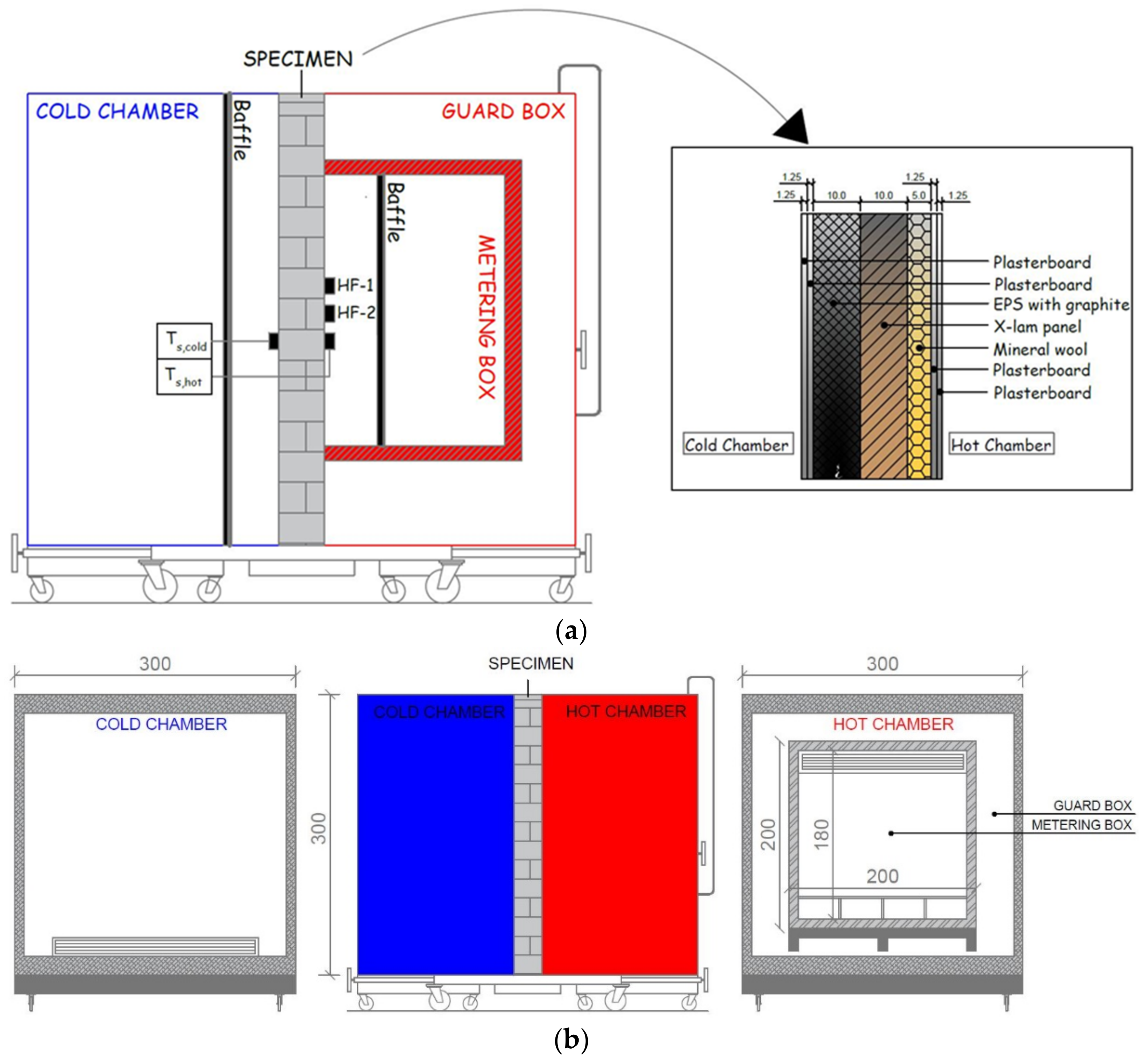
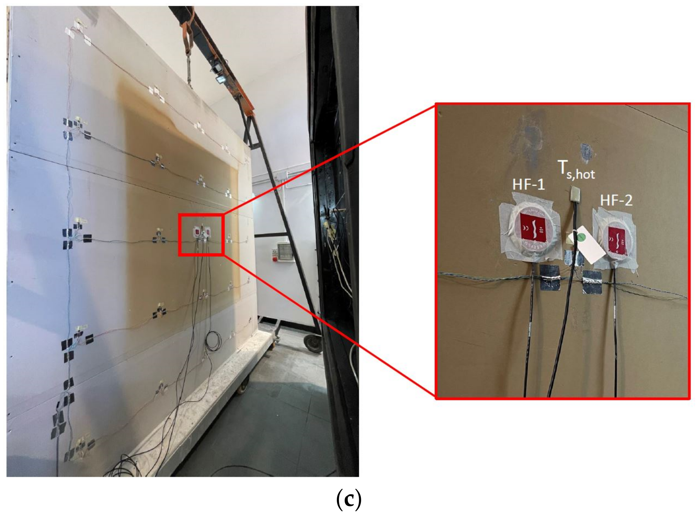
2.2. Experimental Tests via Guarded Hot Box

The steady state thermal performance of buildings’ components can be examined through laboratory tests where a Guarded Hot Box can be employed, making it possible to investigate real-size structural elements subject to established thermal boundary conditions. The Hot Box instrumentation consists of machine control systems able to manage the thermal conditions inside the hot and cold chambers, air and surface temperature sensors, heat flux sensors, and logging systems [32]. The Guarded Hot Box method is an actual scale test. It allows for recreating steady-state and controlled conditions, representative of the buildings’ standard values, and determining the flux through the specimen. These specific conditions are set in accordance with ISO 8990 [33]. Primarily, the recommendations deal with thermal uniformity, constant air flows, and adiabatic conditions for the metering chamber.

The Standard provides some useful suggestions to orientate the design. Most of them concern the thermal homogeneity in the metering zone, with some indications about the range of requested values. Furthermore, the average temperature difference between the hot and cold chambers must be around 20 °C with a respective value close to the standard condition. The GHB removes all meteorological variances, including solar radiation and variable wind speeds experienced by in-situ tests.

Once the temperature difference between the chambers has been set, the apparatus is able to reach and maintain constant thermal conditions over time. Once stationary conditions have been reached, heat fluxes and air and surface temperatures can be measured, and the U-value of the specimen can be obtained.

2.3. In Situ Thermal Transmittance Measurements

The heat flux transmitted through a building element in steady state, divided by the unit of area and by the difference in temperature between the environments separated from the building element is the definition of the U-value. This heat transfer coefficient related to masonries can be found by assessing the heat-flow rate crossing a wall measured through a heat-flow sensor, together with data related to the air temperatures on both sides of the building element, in accordance with the standard ISO 9869-1 [34]. The best conditions for assessing U-values are represented by stable temperatures over time on both sides of the element, that is, in stationary conditions. Nevertheless, stationary conditions do not exist when the measurements are in situ. In practice, to overcome this issue, heat fluxes and temperatures need to be monitored over an adequately long time, thus considering their average values. The thermal conductance or thermal transmittance of a wall can be achieved by dividing the average heat flow density by the average temperature difference, considering a sufficiently long timespan. This value approximates the actual value if the succeeding conditions are satisfied: (i) the element heat content is the same at the end and the beginning of the test (similar temperatures and similar moisture distribution); (ii) direct solar radiation does not impact the heat flow sensor; (iii) the thermal conductivity of the investigated component does not change during the measurement. Misleading findings can be achieved if these three conditions are not satisfied.

Regarding the heat-flow meter sensor installation, positions with exposure to direct solar radiation should be avoided, and north-facing walls are desired. Significant heat flows allow for more accurate measurements. Strongly cooled or intensely heated spaces are ideal measurement places. It can be considered to temporarily activate heaters or air conditioning for an appropriate measurement. Areas with local cold bridges should be avoided, and a preliminary survey through infrared cameras is recommended.

ISO 9869-1 specifies that, by comparing theoretical and experimental values, differences higher than 20% can be associated with: inappropriate materials thermal conductivity values, inappropriate surface heat transfer coefficient values, tests conducted under poor thermal conditions, phase changes (such as freezing, thawing or moisture), the environmental temperatures used for the calculation are not those measured.

2.4. Methodology

The aim of this work is to evaluate how temperature differences between the surfaces of a wall affect heat flux measurements. The experimental setup is based on the GHB apparatus and a specimen wall, with known stratigraphy, interposed between the hot and the cold chambers. Increasing temperature differences, from 2 °C to 20 °C, have been imposed between the faces of the sample wall. Setpoint temperatures are obtained by means of electric resistances, in the hot chamber, and an air-to-air refrigeration unit, in the cold chamber. Therefore, thanks to the controlled and stationary conditions provided by the GHB, heat flux and surface temperatures measurements have been performed. A representation of the experimental setup and the sample wall is shown in Figure 1. The sample wall, composed of an X-lam bearing element, double insulation, and plasterboard, has a theoretical U-value equal to 0.176 W/m²K. The thermophysical properties of the materials that make up the stratigraphy are listed in

Table 1. Thermophysical properties of the materials used for the specimen wall.

Layer	Thermal Conductivity [W/mK]	Mass Density [kg/m3]	Specific Heat Capacity [J/kgK]
Plasterboard	0.210	900	1000
EPS with graphite	0.031	32	1350
X-lam panel	0.130	470	1600
Mineral wool	0.039	135	850

.

As shown in Figure 1, the experimental tests were carried out with a measuring apparatus composed of two equal heat flux sensors (characterized by a thermal resistance of $71\times {10}^{-4}{ \mathrm{m}}^2\mathrm{K}/\mathrm{W}$) connected to a datalogger, positioned on the wall surface facing the hot chamber, and two surface temperature probes (also in this case connected to the same datalogger) installed on the hot and on the cold side of the wall, respectively. The technical data of the measuring instruments are shown in

Table 2. Technical descriptions of the measuring instrument.

Instrument	Manufacturer and Model	Measuring Range
Datalogger	LSI Lastem M-Log ELO008	−300 to +1200 mV
Heat flux sensor	Hukseflux HFP01	−2000 to 2000 W/m2
Temperature probes (Surface)	LSI Lastem EST124-Pt100	−50 to +70 °C

(the same measuring instruments have already been used by the authors in another scientific work [10]).

The ten different experimental tests were carried out, in a continuous way, keeping fixed the set point temperature in the hot chamber (20 °C is a reference value for rooms heated during winter seasons according to the Italian Standard UNI TS 11300-1 [35]) and varying the temperature in the cold chamber, from 18 °C to 0 °C with decreasing steps of 2 °C (in this way simulating increasingly severe winter conditions). For each imposed temperature difference, in order to reach steady state conditions, the experimental campaign had a duration of at least 72 h with a sampling time of 10 min [21], and data related to the most thermally stable 24 h were used to compute the thermal conductance of the sample wall. Thus, the experimental analysis had a total duration of about one month.

Following the standard ISO 9869 [34], the measured data were processed applying the “Average Method”. Therefore, the conduction thermal resistance (R_cond), the thermal conductance, and the thermal transmittance of the wall were obtained by applying the following equations:

$$R_{cond}=\frac{{{\displaystyle \sum }}_{j=1}^n\left(T_{si,j}-T_{se,j}\right)}{{{\displaystyle \sum }}_{j=1}^n{q}_j} \left[\frac{{\mathrm{m}}^2\mathrm{K}}{\mathrm{W}}\right]$$

(5)

$$C=\frac{{{\displaystyle \sum }}_{j=1}^n{q}_j}{{{\displaystyle \sum }}_{j=1}^n\left(T_{si,j}-T_{se,j}\right)} \left[\frac{\mathrm{W}}{{\mathrm{m}}^2\mathrm{K}}\right]$$

(6)

$$U=\frac{1}{R_{tot}}=\frac{1}{R_{si}+R_{cond}+R_{se}} \left[\frac{\mathrm{W}}{{\mathrm{m}}^2\mathrm{K}}\right]$$

(7)

Holman’s method [36] was employed to analyze the propagation of uncertainty of the experimental data obtained for conductance and transmittance values. Based on this method, the uncertainty arising from a set of measurements is determined by the uncertainties of the primary measurements. So, if (z) is a function of the independent variables (x₁, x₂, …, x_n) having uncertainties (w₁, w₂, …, w_n), respectively, the uncertainty in the result (w_z) can be found by applying the following formula:

$$w_z={\left[\left({\left(\frac{\delta z}{\delta x_1}·w_1\right)}^2+{\left(\frac{\delta z}{\delta x_2}·w_2\right)}^2+\dots +{\left(\frac{\delta z}{\delta x_n}·w_n\right)}^2\right)\right]}^{1/2}$$

(8)

2.5. Limitations

Despite the interesting results obtained during the experimental campaign proposed in this work, it is important to point out some potential limitations that would require further investigation:

• tests should also be performed on different walls than the one used;
• the steps of temperature differences variation could be reduced to values less than 2 °C;
• enhanced experimental setup could be used to understand the effects of surface heat transfer coefficients;
• in situ experimental analyses should be conducted to understand how to mitigate less stable thermal conditions due to varying boundary conditions.

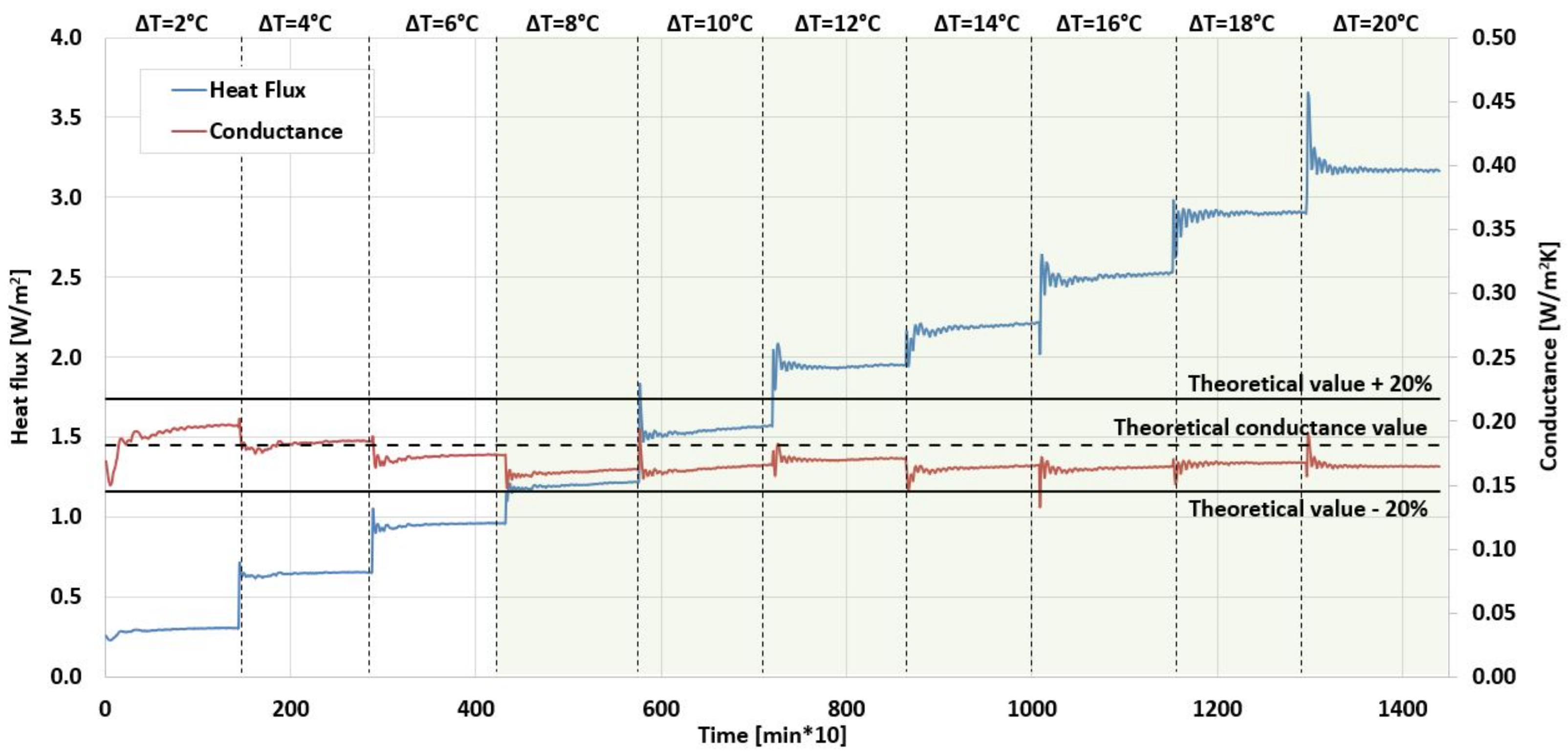
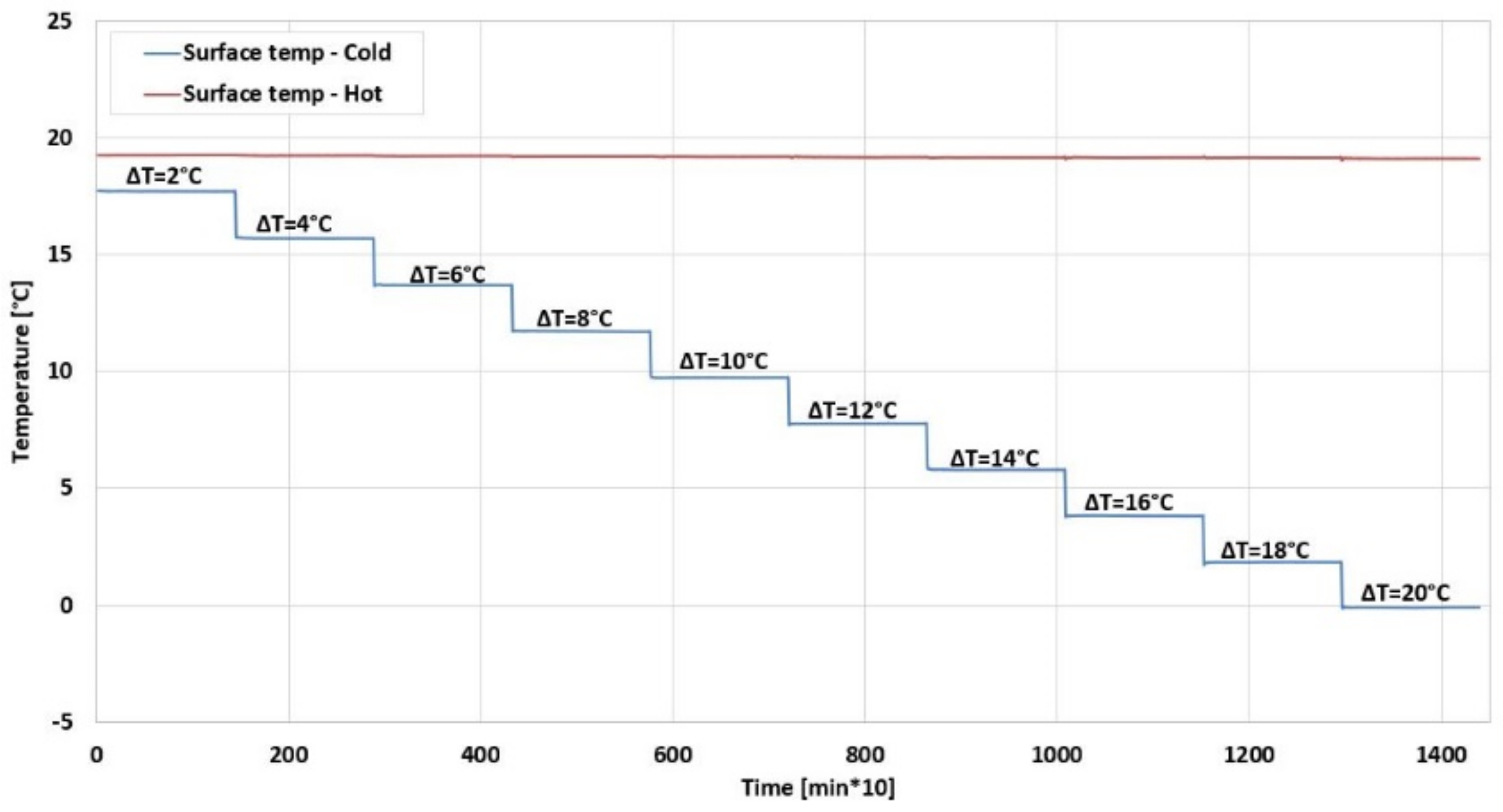
3. Results and Discussion

The experimental results showed that the GHB allows significant thermal stability within the chambers, as shown in Figure 2.

Clearly, the measured heat flux increases with an increasing temperature difference between the chambers. The heat flux values ranged from a minimum average value of 0.290 ± 0.009 W/m², with a temperature difference between the chambers equal to 2 °C, up to the maximum average value of 3.186 ± 0.096 W/m² with a temperature difference between the chambers equal to 20 °C. The mean heat flux values obtained for all the tests are summarized in

Table 3. Average surface temperatures and heat flux obtained for the different tests.

Temperature Difference [°C]	Average Internal Surface Temperature [°C]	Average External Surface Temperature [°C]	Average Heat Flux [W/m2]
2	19.3 ± 0.1	17.7 ± 0.1	0.290 ± 0.009
4	19.3 ± 0.1	15.7 ± 0.1	0.645 ± 0.019
6	19.2 ± 0.1	13.7 ± 0.1	0.951 ± 0.029
8	19.2 ± 0.1	11.7 ± 0.1	1.197 ± 0.036
10	19.2 ± 0.1	9.7 ± 0.1	1.543 ± 0.046
12	19.2 ± 0.1	7.8 ± 0.1	1.945 ± 0.058
14	19.2 ± 0.1	5.8 ± 0.1	2.182 ± 0.065
16	19.2 ± 0.1	3.8 ± 0.1	2.503 ± 0.075
18	19.2 ± 0.1	1.8 ± 0.1	2.893 ± 0.087
20	19.1 ± 0.1	−0.1 ± 0.1	3.186 ± 0.096

.

The experimental setup, characterized by controlled and stable thermal conditions, allowed to obtain consistent thermal conductance values even for low temperature differences between the two surfaces of the sample wall. Figure 3 shows the average heat flux measured with the two sensors and the thermal conductance for the different thermal boundary conditions. It is worth noting that the experimental thermal conductance has values close to the theoretical one (equal to 0.181 W/m²K) and is always within the tolerance range of ±20% with respect to the theoretical value [34]. The green area shown in Figure 3 (starting from a temperature difference of 8 °C to 20 °C) allows for identifying the thermal boundary conditions leading to thermal conductance stabilization.

Assuming the inner and outer surface thermal resistances values equal to 0.13 m²K/W and 0.04 m²K/W [37], the thermal transmittance can be determined for the different experimental configurations. Figure 4 shows the results found in terms of thermal transmittance. Even for low temperature differences between the sample wall faces, but very stable thermal conditions, useful results were obtained. However, it is worthy to stress that the results obtained in terms of U-value derive from internal and external surface heat transfer coefficients not calculated from experimental measurements carried out in the chambers but in the function of the reference values suggested by ISO 6946. Consequently, it is possible to affirm that C-values are easier to compare than U-values, because surface heat transfer resistances may vary and are often quite far from the standard ones adopted for calculations. Systematic underestimates found for large temperature differences may be due to this.

Finally, comparing the experimental thermal transmittance values with the theoretical value (equal to 0.176 W/m²K), it is worth noting that a percentage variation always lower than 10% is obtained, except for the case with a temperature difference equal to 8 °C, in which the percentage variation is slightly higher and equal to 11.4%.

Table 4. Thermal transmittance values and percentage variations for the different cases.

Temperature Difference [°C]	U-Value [W/m2K]	Percentage Variation * [%]
2	0.184 ± 0.018	4.56
4	0.177 ± 0.009	0.76
6	0.167 ± 0.007	−4.85
8	0.156 ± 0.006	−11.44
10	0.159 ± 0.005	−9.74
12	0.166 ± 0.005	−5.82
14	0.159 ± 0.005	−9.79
16	0.159 ± 0.005	−9.79
18	0.162 ± 0.005	−7.74
20	0.161 ± 0.005	−8.48

* With respect to the theoretical value equal to 0.176 W/m²K.

shows the experimental thermal transmittance values and the percentage variation with respect to the theoretical value. It is worth noting that even with small temperature differences, but stable thermal conditions guaranteed by laboratory setup, mutually comparable transmittance values can be obtained.

4. Conclusions

This work shows the results of several tests performed to evaluate the impacts on heat flux measurements due to variable temperature differences between the surfaces of a wall. The analysis was performed employing a Guarded Hot Box apparatus, which allowed to obtain stable thermal boundary conditions. The heat flux and surface temperature measurements allowed to estimate C-values and U-values of the specimen wall for different cases characterized by variable temperature differences between the hot and cold chambers.

The experimental analysis provided interesting results, which have shown that stable thermal conditions allow the obtainment of valid heat flux measurements and, consequently, thermal transmittance values, even for low temperature differences between the hot and cold surfaces of a wall. Even with a temperature difference equal to 2 °C, a thermal transmittance value of 0.184 ± 0.018 W/m²K is obtained, i.e., a variation of 4.56% with respect to the theoretical value of 0.176 W/m²K. Moreover, with a temperature difference of 20 °C, a value equal to 0.161 ± 0.005 W/m²K was obtained, i.e., a difference equal to −8.48%. However, it is important to highlight that, even in a controlled environment, such as the GHB, the achievement of stationary and stable thermal conditions requires a certain transient period, equal to at least two days.

Starting from the obtained results, this research can be considered the first step of a wider study related to the need for high indoor-outdoor temperature difference for thermal transmittance measurements. Therefore, it is worthy to correlate the obtained preliminary findings to the need for temperature stability during the time when the HFM method is applied for in situ measurements. High temperature gradients are commonly required but rarely occur especially in Mediterranean climatic conditions. Moreover, HFM measurements are frequently performed in buildings characterized by heating systems working for time slots, causing convective and radiative effects that can alter the results. The findings here obtained allow us to confirm that the main issue for HFMs seems to be related to temperature stability along time instead of indoor-outdoor temperature differences. Future developments will concern: (i) tests characterized by small steps in terms of temperature variation and an enhanced experimental setup in order to obtain more accurate results (also in terms of surface heat transfer coefficients), (ii) tests on different specimens, characterized by different stratigraphy, to understand if the same results can be obtained and (iii) measurements performed in actual case studies (known stratigraphy), during periods characterized by low internal-external temperature differences.

References

1. Jones, G.F.; Jones, R.W. Steady-state heat transfer in an insulated reinforced concrete wall: Theory, numerical simulations, and experiments. Energy Build. 1999, 29, 293–305. [Google Scholar] [CrossRef]
2. Haralambopoulos, D.A.; Paparsenos, G.F. Assessing the thermal insulation of old buildings—The need for in situ spot measurements of thermal resistance and planar infrared thermography. Energy Convers. Manag. 1998, 39, 65–79. [Google Scholar] [CrossRef]
3. Nardi, I.; Perilli, S.; de Rubeis, T.; Sfarra, S.; Ambrosini, D. Influence of insulation defects on the thermal performance of walls. An experimental and numerical investigation. J. Build. Eng. 2019, 21, 355–365. [Google Scholar] [CrossRef] [Green Version]
4. Nardi, I.; de Rubeis, T.; Buzzi, E.; Sfarra, S.; Ambrosini, D.; Paoletti, D. Modeling and optimization of the thermal performance of a wood-cement block in a low-energy house construction. Energies 2016, 9, 677. [Google Scholar] [CrossRef] [Green Version]
5. Vereecken, E.; Roles, S. A comparison of the hygric performance of interior insulation systems: A hot box-cold box experiment. Energy Build. 2014, 80, 37–44. [Google Scholar] [CrossRef]
6. Woltman, G.; Noel, M.; Fam, A. Experimental and numerical investigations of thermal properties of insulated concrete sandwich panels with fiberglass shear connectors. Energy Build. 2017, 145, 22–31. [Google Scholar] [CrossRef]
7. Gao, Y.; Roux, J.J.; Teodosiu, C.; Zhao, L.H. Reduced linear state model of hollow blocks walls, validation using hot box measurements. Energy Build. 2004, 36, 1107–1115. [Google Scholar] [CrossRef]
8. Luo, C.; Moghtaderi, B.; Hands, S.; Page, A. Determining the thermal capacitance, conductivity and the convective heat transfer coefficient of a brick wall by annually monitored temperatures and total heat fluxes. Energy Build. 2011, 43, 379–385. [Google Scholar] [CrossRef]
9. Maier, M.; Salazar, B.; Unluer, C.; Taylor, H.K.; Ostertag, C.P. Thermal and mechanical performance of a novel 3D printed macro-encapsulation method for phase change materials. J. Build. Eng. 2021, 43, 103124. [Google Scholar] [CrossRef]
10. de Rubeis, T. 3D-printed blocks: Thermal performance analysis and opportunities for insulating materials. Sustainability 2022, 14, 1077. [Google Scholar] [CrossRef]
11. Desogus, G.; Mura, S.; Ricciu, R. Comparing different approaches to in situ measurement of building components thermal resistance. Energy Build. 2011, 43, 2613–2620. [Google Scholar] [CrossRef]
12. Wang, F.; Wang, D.; Wang, X.; Yao, J. A data analysis method for detecting wall thermal resistance considering wind velocity in situ. Energy Build. 2010, 42, 1647–1653. [Google Scholar] [CrossRef]
13. Ficco, G.; Iannetta, F.; Ianniello, E.; Alfano, F.R.D.; Dell’Isola, M. U-value in situ measurement for energy diagnosis of existing buildings. Energy Build. 2015, 104, 108–121. [Google Scholar] [CrossRef]
14. Meng, X.; Yan, B.; Gao, Y.; Wang, J.; Zhang, W.; Long, E. Factors affecting the in situ measurement accuracy of the wall heat transfer coefficient using the heat flow meter method. Energy Build. 2015, 86, 754–765. [Google Scholar] [CrossRef]
15. Cucumo, M.; Ferraro, V.; Kaliakatsos, D.; Mele, M. On the distortion of thermal flux and of surface temperature induced by heat flux sensors positioned on the inner surface of buildings. Energy Build. 2018, 158, 677–683. [Google Scholar] [CrossRef]
16. Guattari, C.; Evangelisti, L.; Gori, P.; Asdrubali, F. Influence of internal heat sources on thermal resistance evaluation through the heat flow meter method. Energy Build. 2017, 135, 187–200. [Google Scholar] [CrossRef]
17. Gaspar, K.; Casals, M.; Gangolells, M. Influence of HFM thermal contact on the accuracy of in situ measurements of façades’ U-value in operational stage. Appl. Sci. 2021, 11, 979. [Google Scholar] [CrossRef]
18. Evangelisti, L.; Guattari, C.; Asdrubali, F. Comparison between heat-flow meter and Air-Surface Temperature Ratio techniques for assembled panels thermal characterization. Energy Build. 2019, 203, 109441. [Google Scholar] [CrossRef]
19. Ahmad, A.; Maslehuddin, M.; Al-Hadhrami, L.M. In situ measurement of thermal transmittance and thermal resistance of hollow reinforced precast concrete walls. Energy Build. 2014, 84, 132–141. [Google Scholar] [CrossRef]
20. Litti, G.; Khoshdel, S.; Audenaert, A.; Braet, J. Hygrothermal performance evaluation of traditional brick masonry in historic buildings. Energy Build. 2015, 105, 393–411. [Google Scholar] [CrossRef]
21. de Rubeis, T.; Evangelisti, L.; Guattari, G.; De Berardinis, P.; Asdrubali, F.; Ambrosini, D. On the influence of environmental boundary conditions on surface thermal resistance of walls: Experimental evaluation through a Guarded Hot Box. Case Stud. Therm. Eng. 2022, 34, 101915. [Google Scholar] [CrossRef]
22. Evangelisti, L.; Guattari, C.; Asdrubali, F. Influence of heating systems on thermal transmittance evaluations: Simulations, experimental measurements and data post-processing. Energy Build. 2018, 168, 180–190. [Google Scholar] [CrossRef]
23. Bienvenido-Huertas, D. Assessing the environmental impact of thermal transmittance tests performed in façades of existing buildings: The case of Spain. Sustainability 2020, 12, 6247. [Google Scholar] [CrossRef]
24. Albatici, R.; Tonelli, A.M. Infrared thermovision technique for the assessment of thermal transmittance value of opaque building elements on site. Energy Build. 2010, 42, 2177–2183. [Google Scholar] [CrossRef]
25. Gori, V.; Elwell, C. Estimation of thermophysical properties from in-situ measurements in all seasons: Quantifying and reducing errors using dynamic grey-box methods. Energy Build. 2018, 167, 290–300. [Google Scholar] [CrossRef]
26. Genova, E.; Fatta, G. The thermal performances of historic masonry: In-situ measurements of thermal conductance on calcarenite stone walls in Palermo. Energy Build. 2018, 168, 363–373. [Google Scholar] [CrossRef]
27. Peng, C.H.; Wu, Z.H. In situ measuring and evaluating the thermal resistance of building construction. Energy Build. 2008, 40, 2076–2082. [Google Scholar] [CrossRef]
28. Cesaratto, P.G.; De Carli, M. A measuring campaign of thermal conductance in situ and possible impacts on net energy demand in buildings. Energy Build. 2013, 59, 29–36. [Google Scholar] [CrossRef]
29. Cesaratto, P.G.; De Carli, M.; Marinetti, S. Effect of different parameters on the in situ thermal conductance evaluation. Energy Build. 2011, 43, 1792–1801. [Google Scholar] [CrossRef]
30. Evangelisti, L.; Guattari, C.; Fontana, L.; Vollaro, R.D.L.; Asdrubali, F. On the ageing and weathering effects in assembled modular facades: On-site experimental measurements in an Italian building of the 1960s. J. Build. Eng. 2021, 45, 103519. [Google Scholar] [CrossRef]
31. Lavine, S.; Incropera, P.; Dewitt, P.; Bergman, T. Fundamentals of Heat and Mass Transfer, 7th ed.; John Wiley & Sons: Hoboken, NJ, USA, 2011; ISBN 13-978-0470-50197-9. [Google Scholar]
32. de Rubeis, T.; Muttillo, M.; Nardi, I.; Pantoli, L.; Stornelli, V.; Ambrosini, D. Integrated measuring and control system for thermal analysis of buildings components in hot box experiments. Energies 2019, 12, 2053. [Google Scholar] [CrossRef] [Green Version]
33. ISO 8990; Thermal Insulation—Determination of Steady-State Thermal Transmission Properties—Calibrated and Guarded Hot Box. ISO: Geneva, Switzerland, 1994.
34. ISO 9869-1; Thermal Insulation—Building Elements—In-Situ Measurement of Thermal Resistance and Thermal Transmittance Heat Flow Meter Method. ISO: Geneva, Switzerland, 2014.
35. UNI/TS 11300-1:2014; Energy Performance of Buildings—Part 1: Determination of the Building’s Thermal Energy Needs for Summer and Winter Air Conditioning (Prestazioni energetiche degli edifice—Parte 1: Determinazione del fabbisogno di energia termica dell’edificio per la climatizzazione estiva ed invernale). UNI: Milan, Italy, 2014.
36. Holman, J.P. Experimental Methods for Engineers, 8th ed.; McGraw-Hill Series in Mechanical Engineering; McGraw-Hill: New York, NY, USA, 2001; ISBN 13-978-0-07-352930-1. [Google Scholar]
37. ISO 6946; Building Components and Building Elements—Thermal Resistance and Thermal Transmittance—Calculation Methods. ISO: Geneva, Switzerland, 2017.
Figure 1. (a) Experimental setup and specimen wall (HF: heat flux meter; Ts: surface temperature probe). (b) Dimensions of the GHB. (c) Picture of the experimental setup. (All the dimensions are in cm).
Energies 15 04746 g001aEnergies 15 04746 g001b
Figure 2. Temperature trends within the GHB for the different cases considered (the acquired data were processed within a graph showing only the last 24 h of measurement for each temperature difference).
Energies 15 04746 g002
Figure 3. Average heat flux and thermal conductance obtained during the tests (the acquired data were processed within a graph showing only the last 24 h of measurement for each temperature difference).
Energies 15 04746 g003
Figure 4. Thermal transmittance values found as a function of the temperature differences obtained in the GHB.
Energies 15 04746 g004