Load Flow and Short-Circuit Methods for Grids Dominated by Inverter-Based Distributed Generation

Abstract

The use of power-electronics-based devices in distribution generation seeks to improve energy quality and reduce costs. The inverter-based distributed generator, that works in different operation modes, has emerged as a promising technology. In a high distributed generation penetration scenario it is important to know the voltage profile and fault information due to the uncertainty in the generator operation and the impact that have on the network. This study aims to use two proposed methods of analysis: for power flow, based on backward/forward sweep method, and short-circuit, based on hybrid impedance matrix, that considers the inverter operation modes and represents each generator as a voltage-controlled current source. The chosen network is the IEEE 34-Node Test Feeder with a generator on each load per phase. The voltage profiles obtained will be validated with a Simulink/Matlab phasorial model. The results show an average error of 2.39% and a gain in voltage profile processing time of 2185.24%, making its use consistent for larger systems.

1. Introduction

Power distribution systems are experiencing a massive increase of distributed generation (DG) based on power electronics with advanced control and capability to manage active and reactive power during normal and abnormal voltage and frequency conditions, e.g., Volt/VAR and frequency-droop. These DG sources, in most cases, have unbalanced phases connected to the grid and, therefore, can make the grid more unbalanced [1].

Updated grid codes and standards, such as the IEEE 1547-2018 [2], for example, try to guide the behavior of DG for normal and abnormal conditions. A grid-connected inverter-based DG (IBDG) source can and will limit its output current to preserve the integrity of the internal components. Therefore, the contribution of IBDG sources for the fault current is quite different when compared to classic rotating machines, and, consequently, many studies have discussed the characteristics and impacts of the short-circuit current of those in the power distribution system [3].

Due to the growing importance of IBDG in the electrical system, recent papers are reporting the effects of these controllers and tend to analyze the voltage profile and fault information to understand the behavior in this scenario [4,5]. These present a significant computational effort, mostly due to the IBDG model and the use of platforms such as DIgSILENT and Simulink, which restrict its use in larger systems with IBDG in every node load. Furthermore, they do not consider the operation of IBDGs according to the voltage ride-through capability, present in recent standards and grid codes.

To fulfill the mentioned gap, this paper proposes two methods: the first is to solve the power flow using an adapted backward/forward sweep (BFS) method and the second for the short-circuit, based on hybrid impedance matrix (HIM). These methods take into consideration the voltage ride-through capability for IBDG following the criteria of IEEE 1547-2018. The IBDG is modeled as a voltage-controlled current source with reactive power capability determined by a Volt/VAR control.

2. Methods Considering Inverter-Based Distributed Generation

In electric power systems, the power flow is a calculation used to identify the steady-state equilibrium points of IBDGs, while the study of the short circuit in systems with IBDG seeks to assess the impact that DGs cause on the network [6]. To relate with the dynamic behavior of the inverter-based resources, by the ride-through requirements and capabilities of inverters, a security-constraint power flow considering the reactive power injection and a calculation model of short-circuit current originating from IBDG sources are proposed. This method satisfies the constraints on the system, such as real and reactive power balance and voltage and current limits, present in the IEEE 1547-2018.

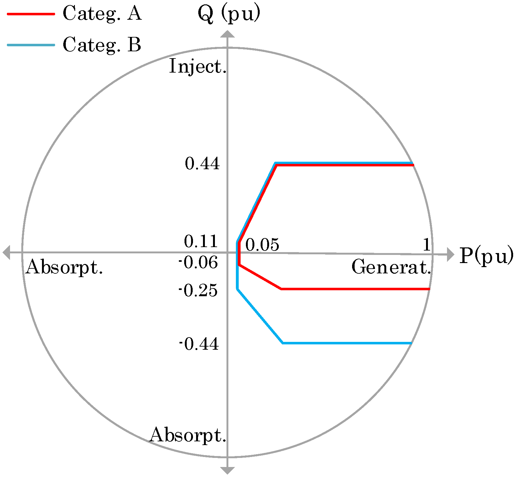
According to IEEE 1547-2018, for a continuous operation region, when the voltage at the point of common coupling (PCC) is between 0.88 and 1.1 times the nominal voltage, the distributed energy resource (DER) can be classified in two categories, related to reactive power capability and voltage regulation performance: Category A and B. The reactive power capability curves are presented in Figure 1.

To respond to abnormal conditions, with voltage values outside the continuous operation region at the PCC, the DER can be classified in three categories: Category I, II, and III (more information in [2]). Among other characteristics, these categories standardize the voltage and frequency ride-through behavior and capabilities of DER for voltage outside the continuous operation region. Despite not indicating the behavior of the DER for this situation, the standard establishes that DER can perform dynamic voltage support (DVS) by providing a rapid reactive power exchange with the network during voltage excursions, and its effectiveness relies on the X/R ratio of the feeder [7]).

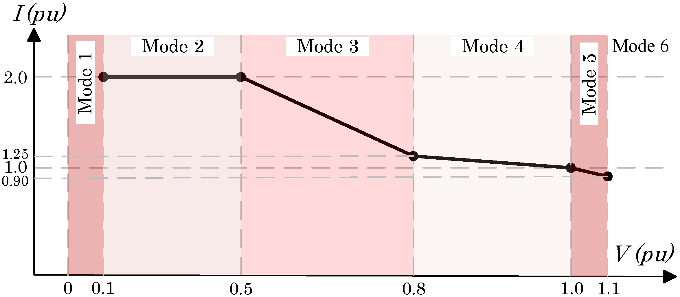
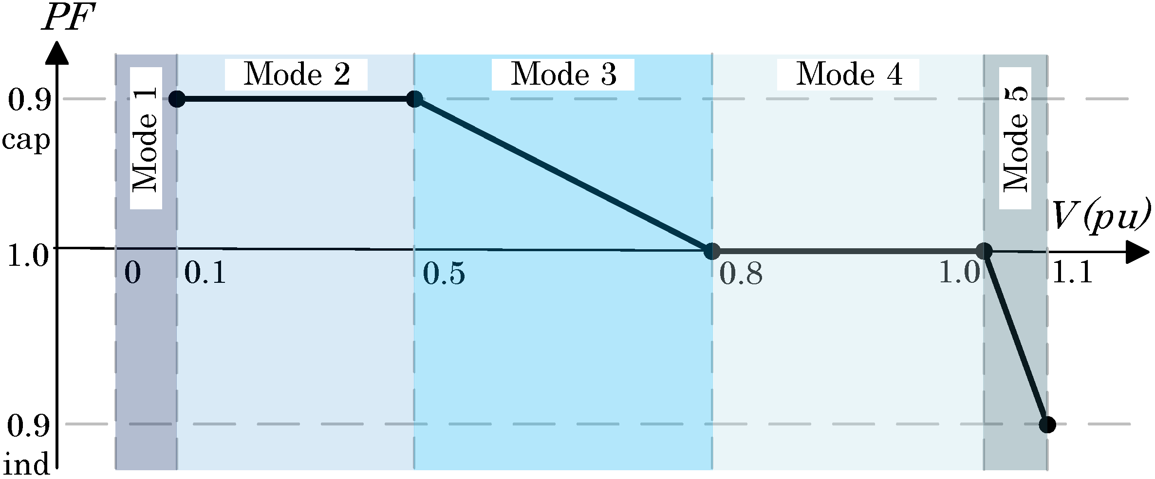
Additionally, the IBDG source needs to limit its output current. Thus, outside the continuous operation region, the IBDG source must limit the current and, for a Volt/VAR control, injects or absorbs reactive power from/to the grid following the reactive power limits presented in Figure 1. To meet a high penetration scenario, the IBDG source adopted in this paper is classified as Category B and III. Its behavior for the output current and reactive power is presented in Figure 2 and Figure 3, relating voltage to current and power factor ($pf$), respectively, with the operating modes that represent the range of values that these electrical quantities can have under normal and abnormal voltage conditions, meeting the requirements of IEEE 1547-2018.

This paper will focus on the analysis of the pre-fault voltage profile, according to the operation modes of Figure 2 and Figure 3 and Category B of IEEE 1547-2018. A method to perform this calculation will provide a better understanding of the operation modes behavior in systems dominated by IBDG, primary source intermittency, the uncertainty in generator operation, and the IBDG impact during fault [8]. This theme follows the recent pattern of various control strategies and grid synchronization methods to keep up with the stringent regulations imposed by the standards [9,10].

3. The DG Model

The chosen DG model to implement the methods is a voltage-controlled current source because it provides higher processing speed and agile implementation to obtain the power flow and short circuit [11]. This model is depicted in Equation (1), where the electrical quantities provided by the DG are ${{\dot{I}}^{*}}_{D{G}_n}$ as current, $P_{D{G}_n}\angle \varphi$ as the active power, and ${\dot{V}}_n$ as node voltage. The model, during the proposed power flow and short circuit methods, will have its reactive power capability determined by a Volt/VAR control (Figure 2 and Figure 3) to simulate the IBDG behavior.

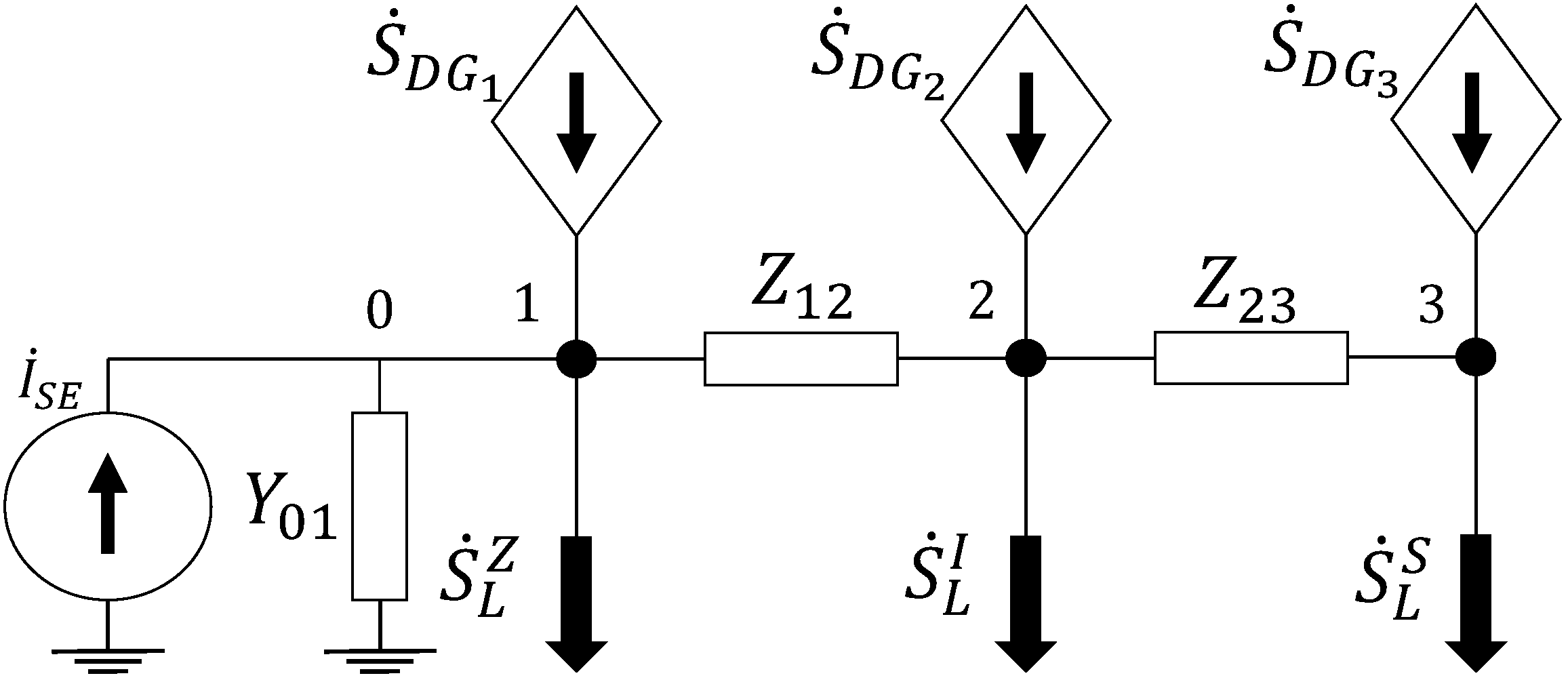
To exemplify: applying this model in a system of a slack bus feeding three loads in series, Figure 4, where the loads ${\dot{S}}_{L_1}$, ${\dot{S}}_{L_2}$, and ${\dot{S}}_{L_3}$ are, respectively, constant impedance (${\dot{S}}_L^Z$), constant current (${\dot{S}}_L^I$), and constant power (${\dot{S}}_L^S$), as shown in (2). The currents flowing in this system have a sum equal to zero, with ${\dot{I}}_{DG}$ being the generated current, ${\dot{I}}_L$ the consumed, and ${\dot{I}}_T$ the transmitted, as shown in (3). Therefore the transmitted power can be written as (4) and as (5), in the matrix form considering each load type.

$$\begin{array}{c}\hfill {{\dot{I}}^{*}}_{D{G}_n}=\frac{P_{D{G}_n}\angle \varphi }{cos\left(\varphi \right)·{\dot{V}}_n}=\frac{S_{D{G}_n}\angle \varphi }{{\dot{V}}_n}\Rightarrow S_{D{G}_n}\angle \varphi ={\dot{V}}_n·{{\dot{I}}^{*}}_{D{G}_n}\end{array}$$

(1)

$$\begin{array}{c}\hfill {\dot{S}}_L={\dot{S}}_{L_1}+{\dot{S}}_{L_2}+{\dot{S}}_{L_3}={{\dot{S}}_L}^Z+{{\dot{S}}_L}^I+{{\dot{S}}_L}^S\end{array}$$

(2)

$$\begin{array}{c}\hfill {\dot{I}}_{DG}-{\dot{I}}_L-{\dot{I}}_T=0\Rightarrow {\dot{I}}_T=Y·\dot{V}={\dot{I}}_{DG}-{\dot{I}}_L\end{array}$$

(3)

$$\begin{array}{c}\hfill \dot{S_T}=\dot{V}·Y^{*}·{\dot{V}}^{*}=\sum _{n=1}^3({\dot{S}}_{D{G}_n}-{\dot{S}}_{L_n})\end{array}$$

(4)

$$\begin{array}{c}\hfill \left[\begin{array}{ccc}{\dot{V}}_1& 0& 0\\ 0& {\dot{V}}_2& 0\\ 0& 0& {\dot{V}}_3\end{array}\right]·Y_{3x3}^{*}\left[\begin{array}{c}{\dot{V}}_1^{*}\\ {\dot{V}}_2^{*}\\ {\dot{V}}_3^{*}\end{array}\right]=\left[\begin{array}{c}{\dot{V}}_1·Y_{01}^{*}+S_{D{G}_1}\angle {\varphi }_1-{\dot{S}}_L^Z·{\dot{V}}_1·{\dot{V}}_1^{*}\\ S_{D{G}_2}\angle {\varphi }_2-{\dot{S}}_L^I·{\dot{V}}_2\\ S_{D{G}_3}\angle {\varphi }_3-{\dot{S}}_L^S\end{array}\right]\end{array}$$

(5)

4. Method for Power Flow

The proposed method for the power flow calculation uses a ladder iterative technique of BFS, considering the different types of node loads and distribution line components, modified for situations with high IBDG penetration, at which each generator is considered as a voltage-controlled current source [12], to obtain the voltage profile. The presented method contemplates the IBDG Category B capability and operation modes, from voltage-power factor curve, under normal and abnormal voltage conditions [13].

The input data are the elements of the lines and the nodes. These are, respectively, composed of the impedance matrices ($Z_l$), characteristics of the transformers and voltage regulators ($\alpha$ and $Z_t$). The nodes inputs are the types and powers of the loads (P and Q) and the capacitors ($Q_{cp}$), the reference voltage (${\dot{V}}_{ref}$), and the active power parameter of each IBDG, expressed by ${\kappa }_A$. The ${\kappa }_A$ value represents how much active power of each load the IBDG is providing, and can be the same for every distribution node in system studies with the same penetration rate.

The ${\kappa }_A$ counterpart is the reactive power parameter, ${\kappa }_R$. This variable means how much reactive power of each load the IBDG is providing. The ${\kappa }_R$ is obtained, as shown in (6), for a system with n nodes, which is limited in (7) according to Category B. In the first iteration, the $pf$ value is 1. With this parameter, the apparent power ${\dot{S}}_n$ of each node is obtained, as presented in (8). The current of each node is obtained using the apparent power from (9) and (10) (where angles are in degrees) and ${\dot{V}}_{ref}$, or the nodal voltage ${\dot{V}}_n$, by equations that depend on the type and configuration of each node. The equations (9) are used for delta configuration loads with constant impedance (${\dot{I}}_{Z_{D_n}}$), constant current (${\dot{I}}_{I_{D_n}}$), and constant apparent power (${\dot{I}}_{S_{D_n}}$). Similarly, Equation (10) is used for wye configuration loads for ${\dot{I}}_{Z_{Y_n}}$, ${\dot{I}}_{I_{Y_n}}$, and ${\dot{I}}_{S_{Y_n}}$, respectively, to obtain the node current.

The parameters obtained above are used to calculate the current ${\dot{I}}_n$ in every line of the system, as shown in (11). In the first iteration, the node voltages are equal to the reference voltage and, after that, the node voltage updated is obtained in (12), considering the transformation ratio ${\alpha }_n$ and impedance $Z_{t_n}$ of transformers and voltage regulators. If the difference between these two voltages are greater than the tolerance, as shown in (13), the process starts again using the last parameter as reference for each node. If not, it starts the stage of adjusting the IBDG curve.

Depending on the voltage obtained, the IBDG $pf$ must be modified, as shown in (14), which represents the operation modes ($M_n$), 1 to 5, of the inverter curve, based on Figure 3. If the $pf$ and node voltage variables do not meet the curves conditions, the new $pf$ value will be inserted in (1), restarting the iterative process. The calculation will remain in this loop until the node voltages and DG power factor are coherent with the IBDG curve parameters.

$$\begin{array}{c}\hfill {\kappa }_{R_{n_{abc}}}^{\prime }=\frac{{\kappa }_{A_{n_{abc}}}·P_{n_{abc}}·(1-p{f}_{n_{abc}})}{p{f}_{n_{abc}}·j·Q_{n_{abc}}}\end{array}$$

(6)

$${\kappa }_{R_{n_{abc}}}=\left\{\begin{array}{c}0.44,{\kappa }_{R_{n_{abc}}}^{\prime }\ge 0.44\hfill \\ {\kappa }_{R_{n_{abc}}}^{\prime },-0.44<{\kappa }_{R_{n_{abc}}}^{\prime }<0.44\hfill \\ -0.44,{\kappa }_{R_{n_{abc}}}^{\prime }\le -0.44\hfill \end{array}\right.$$

(7)

$${\dot{S}}_{n_{abc}}=(1-{\kappa }_{A_{n_{abc}}})·P_{n_{a}bc}+j·(Q_{n_{abc}}-Q_{c{p}_{abc}})·(1-{\kappa }_{R_{n_{abc}}})$$

(8)

$$\begin{array}{c}\hfill {\dot{I}}_{Z_{D_n}}=\left[\begin{array}{c}\frac{{({\dot{S}}_{D_{a_n}}·{{\dot{V}}^{*}}_{a{b}_n})}^{*}-{({\dot{S}}_{D_{c_n}}·{{\dot{V}}^{*}}_{c{a}_n})}^{*}}{{\dot{V}}_{ref}·{{\dot{V}}_{ref}}^{*}}\\ \frac{{({\dot{S}}_{D_{b_n}}·{{\dot{V}}^{*}}_{b{c}_n})}^{*}-{({\dot{S}}_{D_{a_n}}·{{\dot{V}}^{*}}_{a{b}_n})}^{*}}{{\dot{V}}_{ref}·{{\dot{V}}_{ref}}^{*}}\\ \frac{{({\dot{S}}_{D_{c_n}}·{{\dot{V}}^{*}}_{c{a}_n})}^{*}-{({\dot{S}}_{D_{b_n}}·{{\dot{V}}^{*}}_{b{c}_n})}^{*}}{{\dot{V}}_{ref}·{{\dot{V}}_{ref}}^{*}}\end{array}\right],{\dot{I}}_{I_{D_n}}=\left[\begin{array}{c}{\left(\frac{{\dot{S}}_{D_{a_n}}}{|V_{ref}|\angle 30}\right)}^{*}-{\left(\frac{{\dot{S}}_{D_{c_n}}}{|V_{ref}|\angle 150}\right)}^{*}\\ {\left(\frac{{\dot{S}}_{D_{b_n}}}{|V_{ref}|\angle -90}\right)}^{*}-{\left(\frac{{\dot{S}}_{D_{a_n}}}{|V_{ref}|\angle 30}\right)}^{*}\\ {\left(\frac{{\dot{S}}_{D_{c_n}}}{|V_{ref}|\angle 150}\right)}^{*}-{\left(\frac{{\dot{S}}_{D_{b_n}}}{|V_{ref}|\angle -90}\right)}^{*}\end{array}\right],{\dot{I}}_{S_{D_n}}=\left[\begin{array}{c}{\left(\frac{{\dot{S}}_{D_{a_n}}}{{\dot{V}}_{a{b}_n}}\right)}^{*}-{\left(\frac{{\dot{S}}_{D_{c_n}}}{{\dot{V}}_{c{a}_n}}\right)}^{*}\\ {\left(\frac{{\dot{S}}_{D_{b_n}}}{{\dot{V}}_{b{c}_n}}\right)}^{*}-{\left(\frac{{\dot{S}}_{D_{a_n}}}{{\dot{V}}_{a{b}_n}}\right)}^{*}\\ {\left(\frac{{\dot{S}}_{D_{c_n}}}{{\dot{V}}_{c{a}_n}}\right)}^{*}-{\left(\frac{{\dot{S}}_{D_{b_n}}}{{\dot{V}}_{b{c}_n}}\right)}^{*}\end{array}\right]\end{array}$$

(9)

$$\begin{array}{c}\hfill {\dot{I}}_{Z_{Y_n}}=\left[\begin{array}{c}\frac{{({\dot{S}}_{Y_{a_n}}·{{\dot{V}}^{*}}_{Y_{a_n}})}^{*}}{{\dot{V}}_{ref}·{{\dot{V}}_{ref}}^{*}}\\ \frac{{({\dot{S}}_{Y_{b_n}}·{{\dot{V}}^{*}}_{Y_{b_n}})}^{*}}{{\dot{V}}_{ref}·{{\dot{V}}_{ref}}^{*}}\\ \frac{{({\dot{S}}_{Y_{c_n}}·{{\dot{V}}^{*}}_{Y_{c_n}})}^{*}}{{\dot{V}}_{ref}·{{\dot{V}}_{ref}}^{*}}\end{array}\right],{\dot{I}}_{I_{Y_n}}=\left[\begin{array}{c}{\left(\frac{{\dot{S}}_{Y_{a_n}}}{|V_{ref}|\angle 0}\right)}^{*}\\ {\left(\frac{{\dot{S}}_{Y_{b_n}}}{|V_{ref}|\angle -120}\right)}^{*}\\ {\left(\frac{{\dot{S}}_{Y_{c_n}}}{|V_{ref}|\angle 120}\right)}^{*}\end{array}\right],{\dot{I}}_{S_{Y_n}}=\left[\begin{array}{c}{\left(\frac{{\dot{S}}_{Y_{a_n}}}{{\dot{V}}_{a_n}}\right)}^{*}\\ {\left(\frac{{\dot{S}}_{Y_{b_n}}}{{\dot{V}}_{b_n}}\right)}^{*}\\ {\left(\frac{{\dot{S}}_{Y_{c_n}}}{{\dot{V}}_{c_n}}\right)}^{*}\end{array}\right]\end{array}$$

(10)

$$\begin{array}{c}\hfill {\dot{I}}_n={\dot{I}}_{D_n}+{\dot{I}}_{Y_n}-({\dot{Y}}_{a_n}^{*}·{\dot{V}}_{a_n}+{\dot{Y}}_{b_n}^{*}·{\dot{V}}_{b_n}+{\dot{Y}}_{c_n}^{*}·{\dot{V}}_{c_n})\end{array}$$

(11)

$$\begin{array}{c}\hfill {\dot{V}}_{n_{abc}}={\alpha }_t·{\dot{V}}_{s_{abc}}-(Z_{l_{abc}}+Z_{t_{abc}})·{\dot{I}}_n\end{array}$$

(12)

$$\begin{array}{c}\hfill Tolerance:\sum ^n\left(\right|{\dot{V}}_{n_{abc}}^{{}^{″}}|-|{\dot{V}}_{n_{abc}}^{{}^{\prime }}\left|\right)\end{array}$$

(13)

$$p{f}_{n_{abc}}=\left\{\begin{array}{c}0.9,0\le {\left|V\right|}_{n_{abc}}\le 0.1,M_1\hfill \\ {0.9,0.1<\left|V\right|}_{n_{abc}}\le 0.5,M_2\hfill \\ 0.33·{\left|V\right|}_{n_{abc}}+0.73,0.5<{\left|V\right|}_{n_{abc}}\le 0.8,M_3\hfill \\ {1.0,0.8<\left|V\right|}_{n_{abc}}\le 1.0,M_4\hfill \\ -1.22·{\left|V\right|}_{n_{abc}}+2.22,1<{\left|V\right|}_{n_{abc}}\le 1.1,M_5\hfill \end{array}\right.$$

(14)

5. Method for Short Circuit

The proposed short-circuit method uses another ladder iterative method relating the superposition principle and the impedance matrix method [14], but in a hybrid version [15], to calculate the supply of current from each individual IBDG and then perform the sum, obtaining the fault current which will be subjected to the IBDG operation mode. The calculation uses the voltage profile, obtained from the previous method, and fault characteristics: location and type.

The impedance matrix method uses the line Equations (10) and (11), thus considering a system with n nodes and x being the fault point; the calculation starts with the determination of the $Z_{{eq}_{abc}}$ impedance matrix, from source to shorting point, obtained by calculating the Thevenin equivalent impedance, $Z_{{Th}_x}$, with the sum of the line impedances $Z_{l_{ab{c}_n}}$, as shown in (15). The post-fault source voltage, ${\dot{V_s}}_{abc}$, will be obtained from (16), where ${\dot{I}}_{f_{abc}}$ is the fault current, $Z_{f_{abc}}$ is the fault impedance, ${\dot{V}}_{f_{ab{c}_x}}$ is the fault point voltage, ${\dot{V}}_{f_{g_x}}$ is the reference line to ground fault voltage, and ${\dot{V}}_{{GD}_{abc}}$ is the voltage of one of the generators of the n-node system.

Setting (16) in the matrix format, using the simplified product of the system admittance, given by Y, according to (17), we obtain (18), where the C variables vary from 0, −1 or 1, depending on the fault type, as shown in (19), which can be reduced to a three-element operation, represented by $\dot{I}{P}_{abc}$ (post fault source current), C, and ${\dot{X}}_{f_{abc}}$ (voltage and current fault), as shown in (20).

As informed, this method uses the superposition principle to calculate the supply of current coming from the IBDGs individually and then perform the sum in (21). The result will be subjected to the tolerance, (22), to check if the quantities deviate according to a predefined limit. Thus, when obtaining the output quantities present in the vector ${\dot{X}}_{f_{abc}}$, ${\dot{I}}_{f_{abc}}$ and ${\dot{V}}_{f_{abc}}$ are forwarded to the system of equations in (23) to obtain the operation mode of each IBGD, based on Figure 2.

If these electrical quantities are outside the range of the curve, it is necessary to disconnect the DG from the system, conditions present in mode 6 ($M_6$), since the generator behavior will be outside the operation range defined by the standard [16]. The system remains in loop until the mode does not change and the values obtained are within the defined tolerance. If these constraints are not met, the algorithm returns to the fault current calculation.

$$\begin{array}{c}\hfill Z_{e{q}_{{abc}_n}}=Z_{T{h}_n}+\sum ^n{Z}_{l_{ab{c}_n}}\end{array}$$

(15)

$$\begin{array}{c}\hfill {\dot{V}}_{s_{abc}}=(Z_{e{q}_{abc}}+Z_{f_{abc}})·{\dot{I}}_{f_{abc}}+{\dot{V}}_{f_{ab{c}_x}}+{\dot{V}}_{{GD}_{abc}}\end{array}$$

(16)

$$\begin{array}{c}\hfill Y={(Z_{e{q}_{abc}}+Z_{f_{abc}})}^{-1}\end{array}$$

(17)

$$\begin{array}{c}\hfill \left[\begin{array}{c}\dot{I}{P}_a\\ \dot{I}{P}_b\\ \dot{I}{P}_c\\ 0\\ 0\\ 0\\ 0\\ 0\\ 0\end{array}\right]=\left[\begin{array}{ccccccccc}1& 0& 0& 0& 0& 0& Y_{1,1}& Y_{1,2}& Y_{1,3}\\ 0& 1& 0& 0& 0& 0& Y_{2,1}& Y_{2,2}& Y_{2,3}\\ 0& 0& 1& 0& 0& 0& Y_{3,1}& Y_{3,2}& Y_{3,3}\\ -Z_{f_a}& 0& 0& 1& 0& 0& -1& 0& 0\\ 0& -Z_{f_b}& 0& 0& 1& 0& 0& -1& 0\\ 0& 0& -Z_{f_c}& 0& 0& 1& 0& 0& -1\\ C_{7,1}& C_{7,2}& C_{7,3}& 0& 0& 0& C_{7,7}& C_{7,8}& C_{7,9}\\ C_{8,1}& C_{8,2}& C_{8,3}& 0& 0& 0& C_{8,7}& C_{8,8}& C_{8,9}\\ C_{9,1}& C_{9,2}& C_{9,3}& 0& 0& 0& C_{9,7}& C_{9,8}& C_{9,9}\end{array}\right]·\left[\begin{array}{c}{\dot{I_f}}_a\\ {\dot{I_f}}_b\\ {\dot{I_f}}_c\\ {\dot{V_f}}_{a_x}\\ {\dot{V_f}}_{b_x}\\ {\dot{V_f}}_{c_x}\\ {\dot{V}}_{g_{a_x}}\\ {\dot{V}}_{g_{b_x}}\\ {\dot{V}}_{g_{c_x}}\end{array}\right]\end{array}$$

(18)

$$1:\left\{\begin{array}{c}A;C_{7,2},C_{8,3},C_{9,7}=1\hfill \\ B;C_{7,1},C_{8,3},C_{9,8}=1\hfill \\ C;C_{7,1},C_{8,2},C_{9,9}=1\hfill \end{array}\right. 2:\left\{\begin{array}{c}AB;C_{7,1},C_{7,2},C_{8,3},C_{9,7}=1,C_{8,9}=-1\hfill \\ BC;C_{8,1},C_{7,2},C_{7,3},C_{8,9}=1,C_{9,9}=-1\hfill \\ CA;C_{7,1},C_{7,3},C_{8,1},C_{9,7}=1,C_{9,9}=-1\hfill \end{array}\right. 3:\left\{\begin{array}{c}{C}_{7,7},C_{8,8},C_{9,9}=1\hfill \end{array}\right.$$

(19)

$$\begin{array}{c}\hfill {\dot{X}}_{f_{abc}}=C^{-1}·\dot{I}{P}_{abc}\end{array}$$

(20)

$$\begin{array}{c}\hfill {\dot{I}}_{f_{abc}}=\sum ^n({\dot{I}}_{f_x}+{\dot{I}}_{f_{G{D}_{n_{abc}}}})\end{array}$$

(21)

$$\begin{array}{c}\hfill Tolerance:\sum ^n({|{\dot{I}}_f}_{n_{abc}}^{{}^{″}}|-|{{\dot{I}}_f}^{{}^{\prime }}{}_{n_{abc}}\left|\right)\end{array}$$

(22)

$$\left|{\dot{I}}_{f_{abc}}\right|=\left\{\begin{array}{c}0,0\le |{\dot{V}}_{f_{abc}}|\le 0.1,M_1\hfill \\ 2,0.1<|{\dot{V}}_{f_{abc}}|\le 0.5,M_2\hfill \\ -2.5·|{\dot{V}}_{f_{abc}}|+3.25,0.5<|{\dot{V}}_{f_{abc}}|\le 0.8,M_3\hfill \\ -1.25·|{\dot{V}}_{f_{abc}}|+2.25,0.8<|{\dot{V}}_{f_{abc}}|\le 1.0,M_4\hfill \\ -1·|{\dot{V}}_{f_{abc}}|+2,1<|{\dot{V}}_{f_{abc}}|\le 1.1,M_5\hfill \\ 0,|{\dot{V}}_{f_{abc}}|>1.1,M_6\hfill \end{array}\right.$$

(23)

6. Flowchart of the Proposed Methods

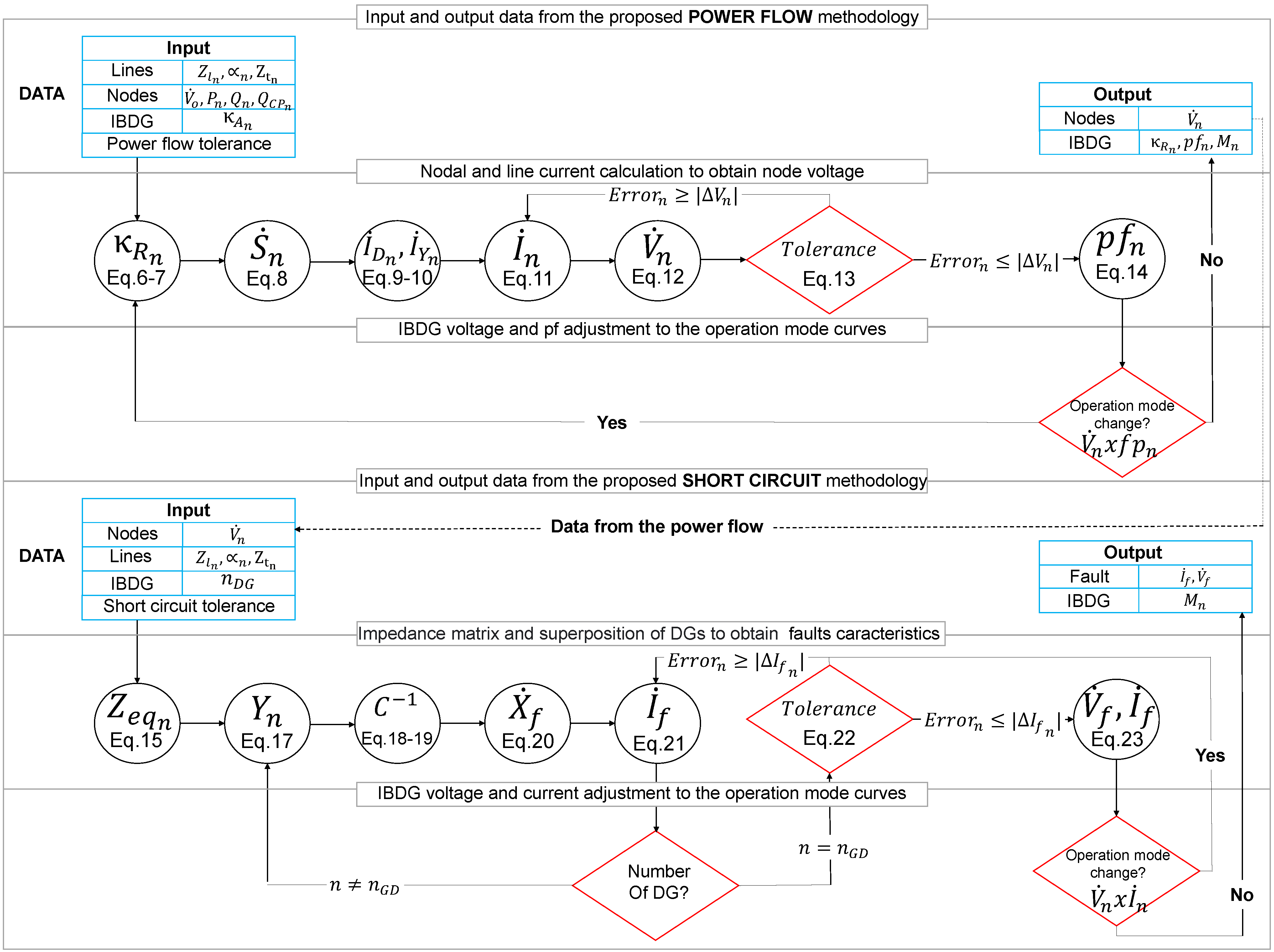
The flowchart of Figure 5 is divided into two steps, the first being for the calculation of the power flow and the second for the short circuit. Each step represents the method presented in Section 3 and Section 4. Each one has the three cycles: input and output of data, calculation of the power flow or the short circuit, and adjustment of the voltage and $pf$, or current, node values based on the operation curves of the IBDG.

For the power flow, in the first stage of the first cycle, the data of the elements of lines and nodes, as well as the DGs and the calculation tolerance, are inserted, which then, in the second cycle, are used to calculate the ${\kappa }_R$ of each node with generation and, consequently, the node power and current. The BFS method obtains the line currents, and mostly the node voltages, whose tolerance in relation to the previous value is the numerical convergence requirement in this cycle.

In the third cycle, the power factors calculated in the first are compared with the ones obtained in the second, using the operation curves as reference. This parameter is updated if the operation mode changes, restarting the second cycle. Otherwise, the values are sent to data output, which is the second stage of the first cycle, leading to the end of the process and sending the pre-fault voltage for the short-circuit calculation step.

For the short circuit, similar to the previous, the first cycle handles the data input: using the output voltage and system characteristics, nodes and lines, from the previous step. In the second cycle, the impedance matrix is obtained and used to build the system admittance, using the fault type, another input data. In this cycle, the fault electrical quantities are obtained as well as the current contribution from the DGs, by superposition method. The current is subjected to a tolerance check and, if not met, a new fault current is calculated, otherwise it goes to the third cycle.

In the final cycle, the fault current and voltage are compared using the operation curves as reference and are updated if the operation mode changes, restarting the second cycle, as in the power flow method. The system will remain in this loop until the conditions are met, withdrawing even the contribution of DGs from the system, to obtain the fault magnitudes and operation mode of the DGs in this scenario.

7. Results and Discussion

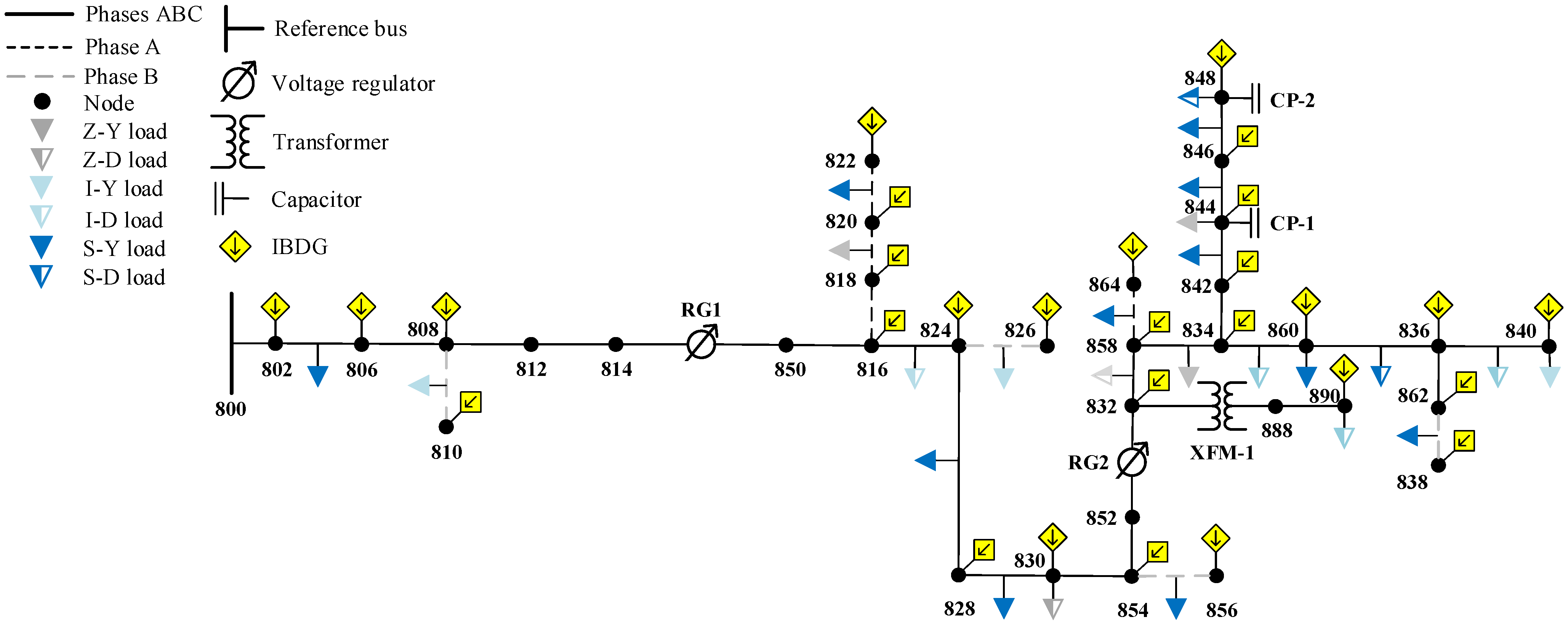
The proposed methods were implemented on the Matlab command line and had as database the IEEE Radial Distribution Test Feeders [17]. Among the available systems, the 34-Node Test Feeder was chosen for being a network with 8 spot and 19 distributed loads, with impedance, current, and constant apparent power, with delta and wye configuration types, in addition to associated capacitors in the nodes, transformers and, voltage regulators on the lines, as presented in Figure 6. To represent a dominated scenario, every node with a load has an IBDG associated, where the source can provide a percentage power, based on the load power.

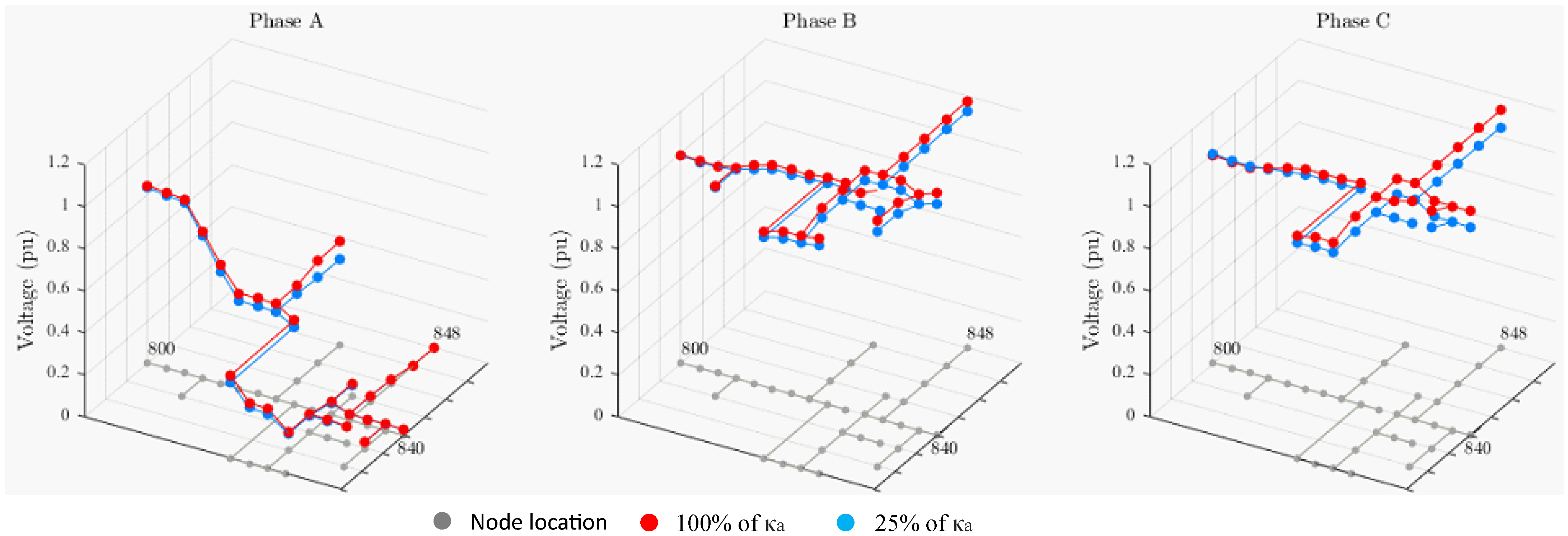
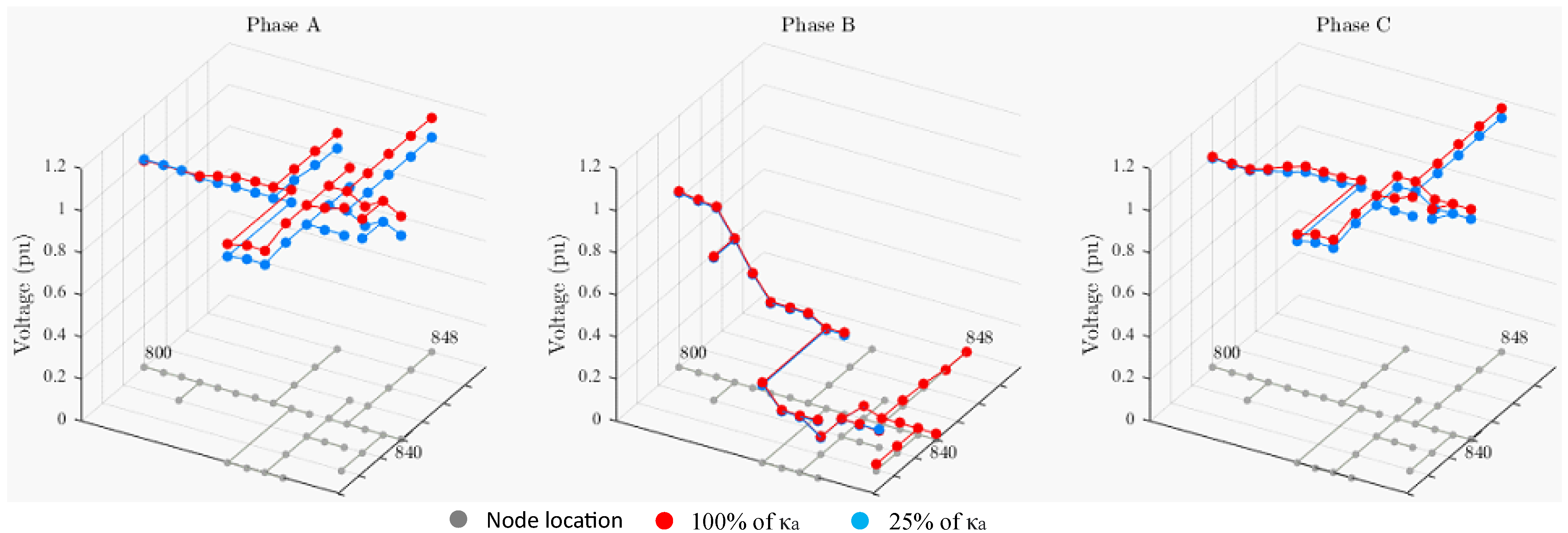
The voltage profile will be shown in a 3D graph and the IBDG operations modes in a graphical circle. This choice allows better visualization of the node voltage and operation mode behavior in relation to the slack bus and the neighboring nodes, in situations of IBDG power variation and fault. In the 3D graph, the zero-axis plane is the topology of the electrical system, in this case, the 34-Node Test Feeder, while the vertical axis is the voltage (in pu) of each node. For a better understanding, some of the nodes located at the ends of the system will be highlighted, in this case, nodes 800, 840, and 848.

The validation of the results obtained by the proposed power flow method come from the comparison with a database using the Simulink model [18], in a scenario with high penetration of IBDG.

7.1. Results for Power Flow

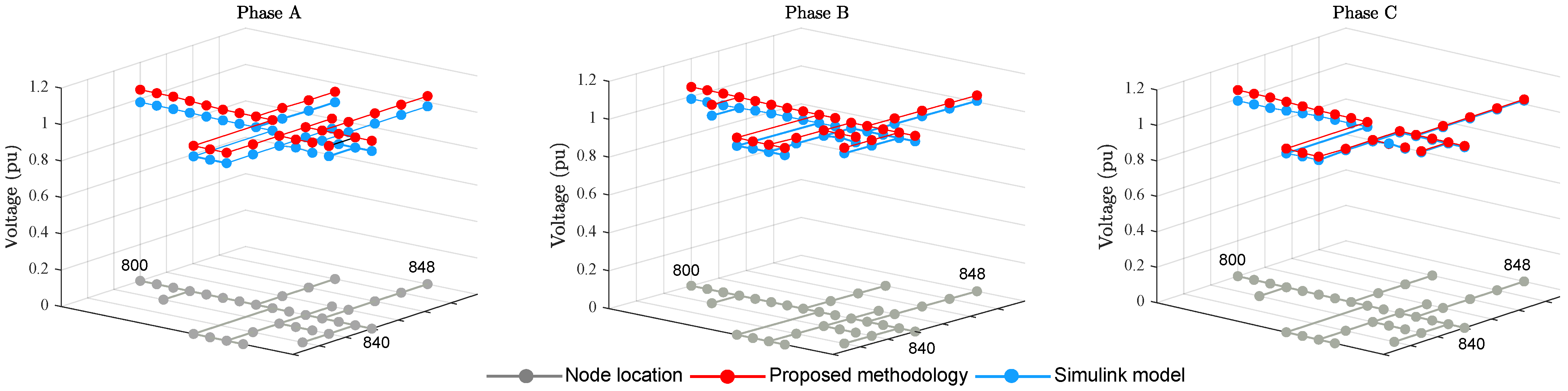
The power flow average values from Simulink simulation [18], with the proposed method, with DGs providing the maximum value of the active power of the loads, in the reference distribution system, are shown in Figure 7.

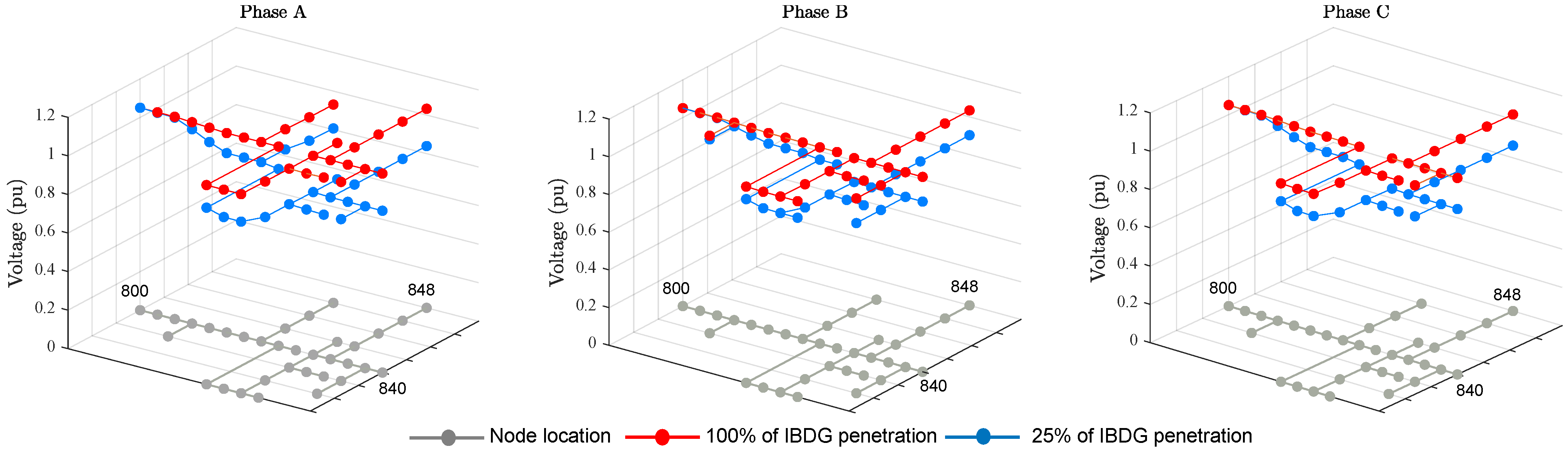
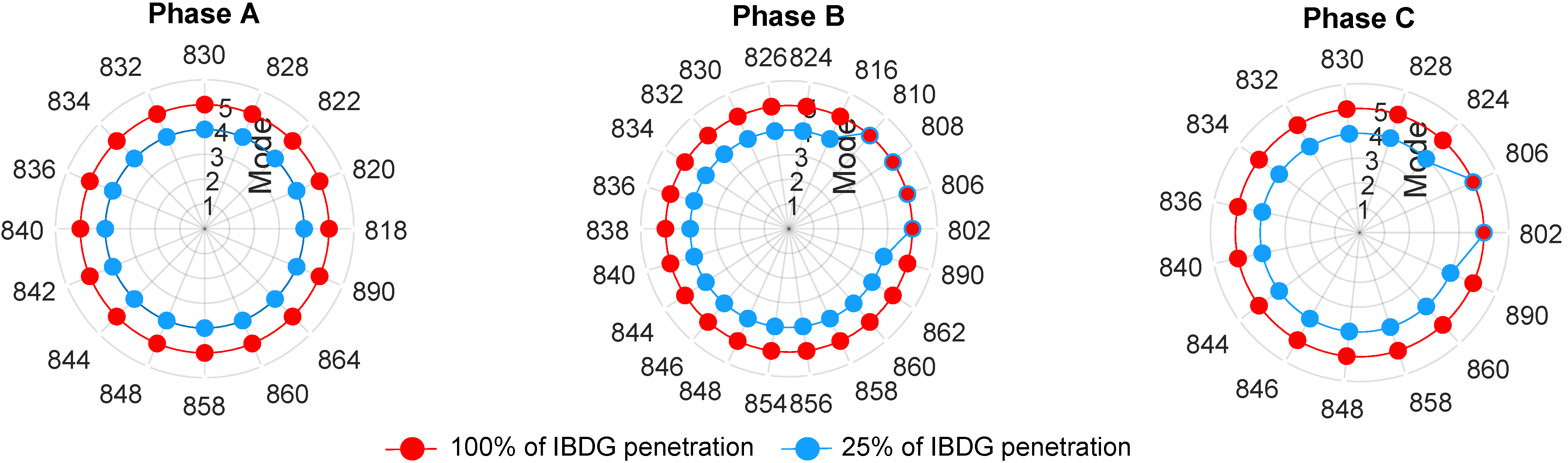
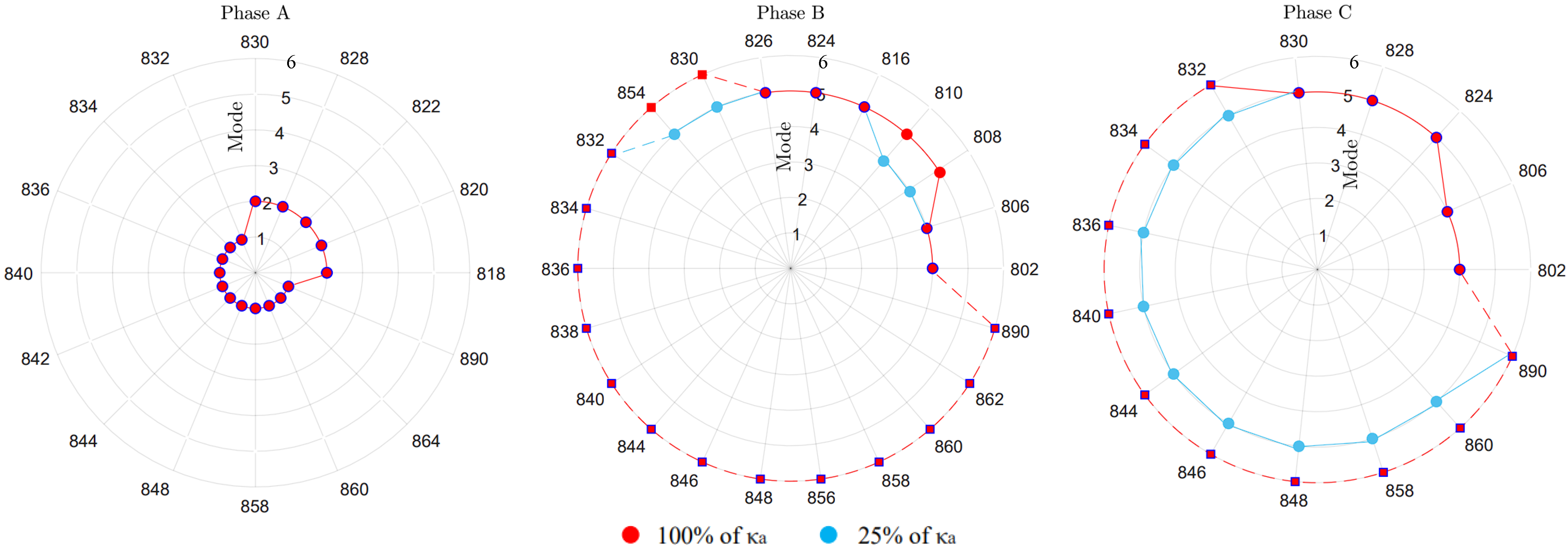
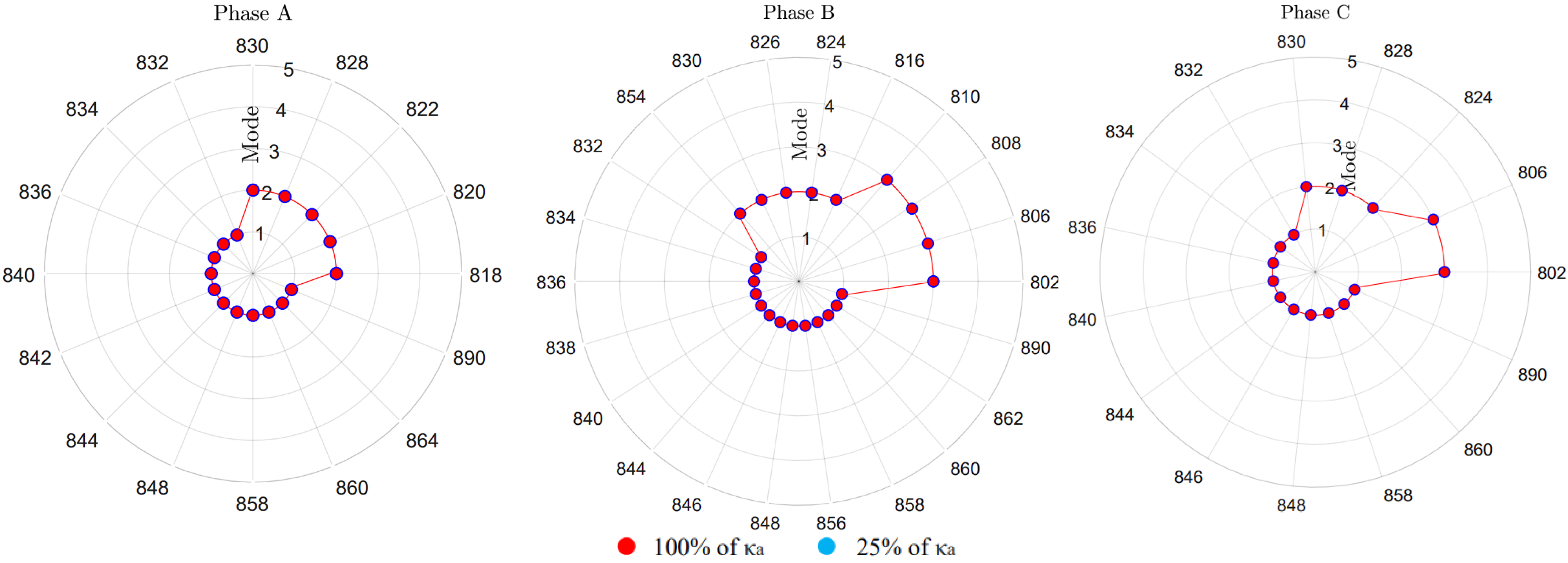
To analyze the behavior of the DGs inverters with the increase of injected active power, the simulation is carried with 25% and 100% of ${\kappa }_A$ for each node with IBDG, as shown in Figure 8 for voltage and operation modes in Figure 9. The $Tolerance$ value chosen was 0.001. The ${\kappa }_R$ of the nodes that have a load, and, as consequence, an IBDG, as shown in

Table 1. ${\kappa }_R$ values in nodes with 100% and 25% of ${\kappa }_A$ for IEEE 34-Node Test Feeder.

${\mathit{\kappa }}_{\mathit{A}}$	100%			25%
Node	Ph-A	Ph-B	Ph-C	Ph-A	Ph-B	Ph-C
802	-	0.1298	0.1155	-	0.0315	0.0276
806	-	0.1295	0.1151	-	0.0308	0.0276
808	-	0.1239	-	-	0.0178	-
810	-	0.1240	-	-	0.0179	-
816	-	0.1361	-	-	-	-
818	-	0.0863	-	-	-	-
820	0.0720	-	-	-	-	-
822	0.0699	-	-	-	-	-
824	-	0.1085	0.0924	-	-	-
826	-	0.1062	-	-	-	-
828	0.0995	-	0.0920	-	-	-
830	0.0864	0.0988	0.1032	-	-	-
854	-	0.0986	-	-	-	-
832	0.0936	0.0867	0.0673	-	-	-
858	0.0877	0.0815	0.0632	-	-	-
834	0.0818	0.0837	0.0653	-	-	-
842	0.0737	-	-	-	-	-
844	0.4400	0.4400	0.4400	-	-	-
846	-	0.0909	0.0610	-	-	-
848	0.0062	0.0107	0.0050	-	-	-
860	0.0639	0.0626	0.0578	-	-	-
836	0.0817	0.0808	0.0626	-	-	-
840	0.0640	0.0687	0.0422	-	-	-
862	-	0.0859	-	-	-	-
838	-	0.0857	-	-	-	-
864	0.0809	-	-	-	-	-
890	0.0733	0.0794	0.0602	-	-	-
856	-	0.0987	-	-	-	-

, evaluates whether the category B power capability maximum and minimum parameters were met. In all tests carried out, the proposed method was able to converge and obtain valid output data. The simulation times for the IEEE 34-Node were 1.33, 1.36, 1.80, and 3.93 s, for 25%, 50%, 75%, and 100% of ${\kappa }_A$, respectively.

The average error for the 34-node system between the proposed method and the Simulink model, with a runtime of 85.88 s, considering the voltage from all phases, is 2.39%, considering maximum active power injection (100% ${\kappa }_A$). The lowest error was found in phase B, being 2.18%, which has the greatest number of IBDG. In phases A and C, the errors were 2.46% and 2.70%, respectively. In Figure 8, the change in the voltage profile regarding the increase in penetration of active power by the IBDG is more significant as it moves away from the swing bus to node 810 in phase B and 806 for phase C.

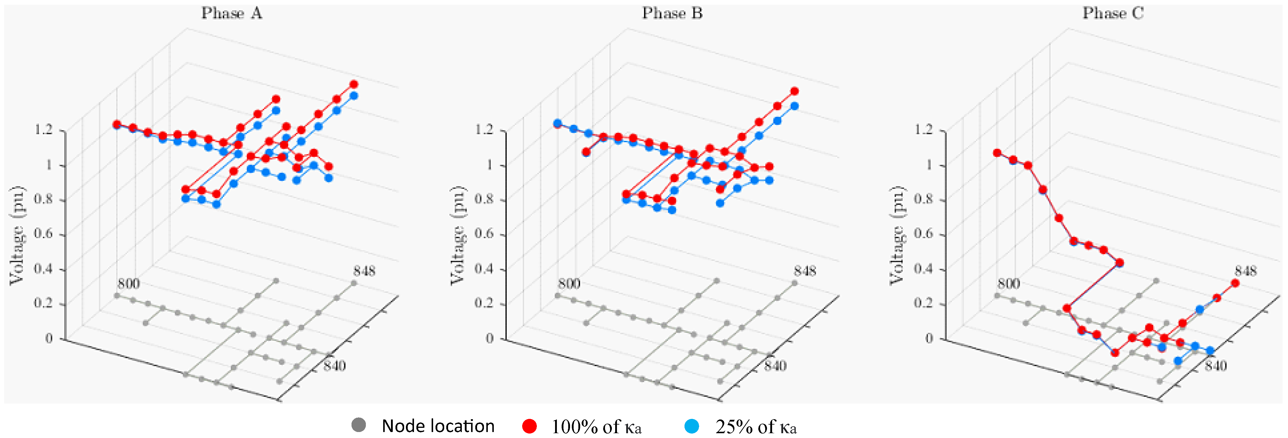
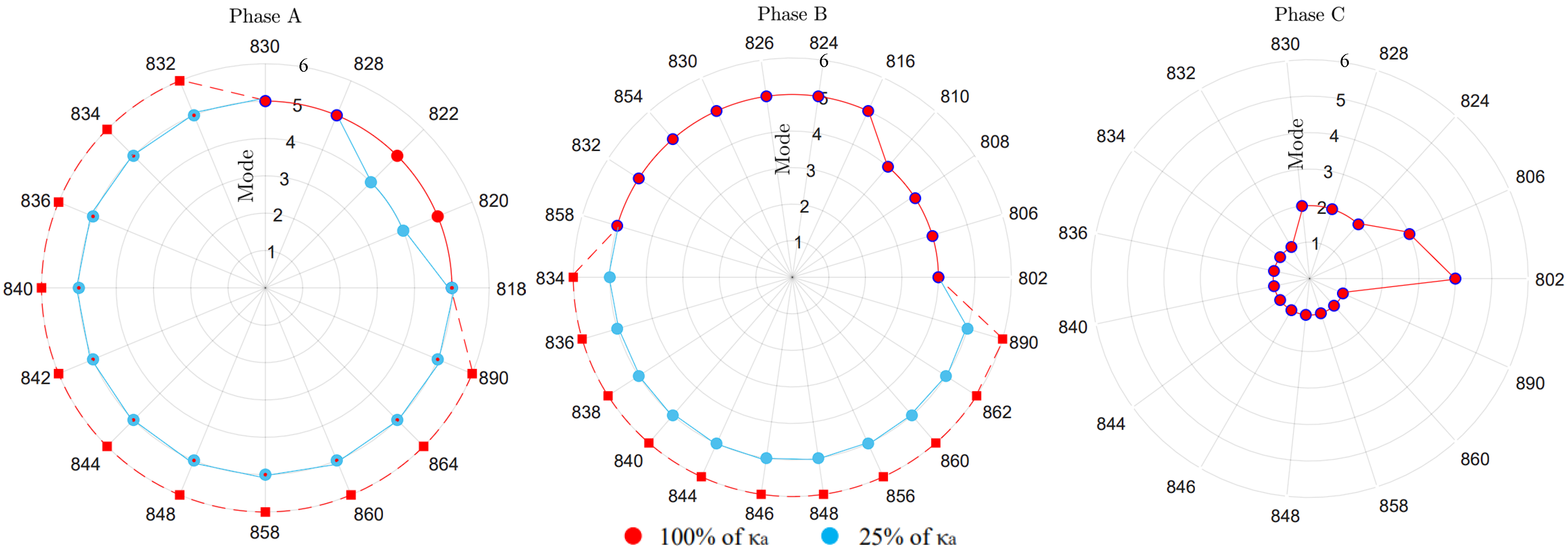
In regard to the operation mode, shown in Figure 9, for 100% of injection of ${\kappa }_A$, all nodes with IBDG were in mode 5. By contrast, for a penetration of 25% of ${\kappa }_A$, with the exception of branches 802–810 for phase B and 802–808 for phase C, all nodes were in operation mode 4. These nodes are closest to the reference bus.

In Table 1, it is shown that the ${\kappa }_R$ met the parameters limits of power capability curves for DERs Category B, indicating that the IBDG operates in mode 5. In mode 4, there is no reactive power injection, and as a result, ${\kappa }_R$ is zero. On node 844, Table 1 indicates that the limit from parameter B for ${\kappa }_R$ was reached, since the values were set at 0.44, as highlighted in red. Such limitation did not prevent the system from converging. Removing this limitation, the ${\kappa }_R$ values for this node become 0.7647, 0.5789, and 0.4568 for phases A, B, and C, respectively, while reducing simulation time to 2.97 s, a decrease of 24% when compared with the restricted one.

7.2. Results for Short Circuit

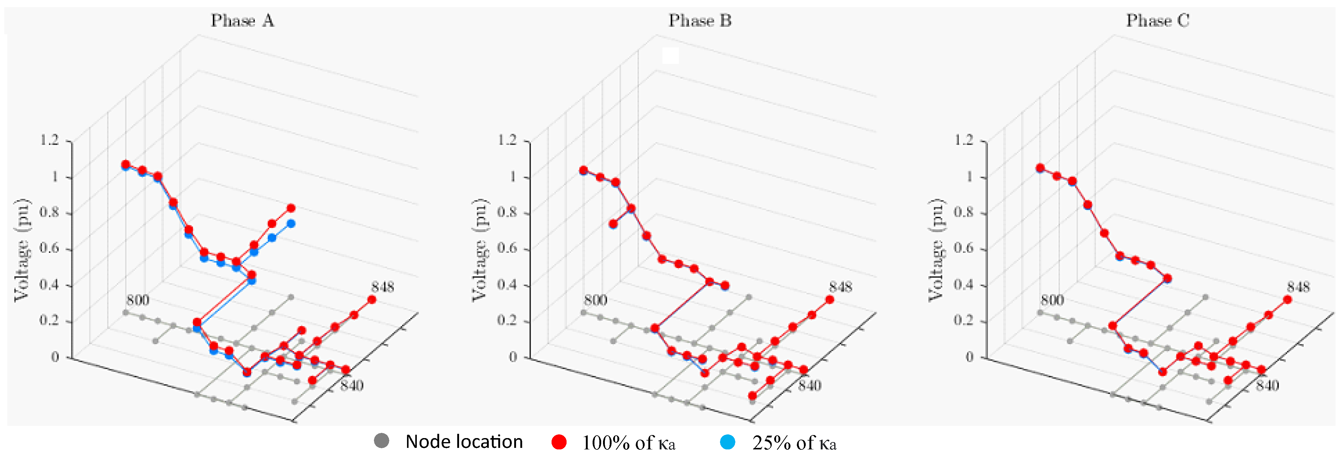
To evaluate the short-circuit behavior in the feeder, the fault was considered at the most distant node, since this scenario causes greater impact in the system. Therefore, the fault will be at node 848 with a $Tolerance$ value of 0.001.

The fault scenarios analyzed will be of the single-phase type for each phase, as it is more common, and three-phase, as it has the highest fault current amplitude. In case of voltage sag as well as current peak, representing operation mode 6, the IBDG will be removed from the feeder.

As in the power flow method, with the considerations informed and also the injection of active power by the IBDGs, the short-circuit current was compared with the data presented in [10] for the scenario with a three-phase fault at node 848.

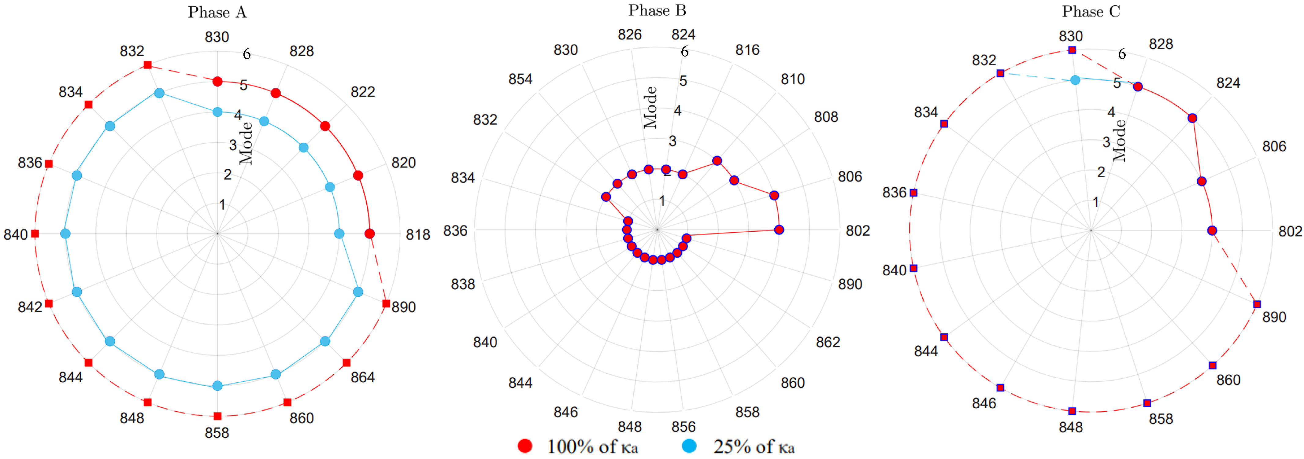
When applying a single-phase fault to phase A of node 848, a voltage dip occurs in the faulted phase. This variation, from the operation mode point of view, does not change with the injection of ${\kappa }_A$, as shown in Figure 10, and is concentrated in mode 1 as it approaches the fault, as demonstrated in Figure 11. In the neighboring phases, extrapolation of the mode occurs mostly in phase B, which holds the highest load, which only occurs in C for maximum ${\kappa }_A$.

Such a fault in phases B and C shows similar behavior, as shown, respectively, in Figure 12 and Figure 13 for phase B and Figure 14 and Figure 15 for phase C, with less voltage dip for IBDGs closer to the reference bus.

For the three-phase fault, there was no mode variation for 25% and 100% of ${\kappa }_A$. However, the effect of the loads being closer to the reference bus becomes more significant, and in this case, farther from the fault, which reduces the effect of voltage sag, as seen in Figure 16 and three operation modes in the branch 802–830, presented in Figure 17.

8. Discussion and Conclusions

The purpose of this paper was to show the implementation of a simulation platform, which applies methods to obtain the power flow and short circuit, in normal and abnormal situations, for electrical energy systems with high penetration of IBDG, considering the limits and operation modes associated with them.

The simulations, mostly in Table 1, showed that for power flow with a minimum power supply (25%), most IBDG nodes operate in mode 4, not injecting reactive power, and with maximum power supply, the reactive power injection limit in Category B is reached at node 844, a situation that must be repeated for high reactive power consumption loads. Such scenario shows that a revision in the limits is a point of analysis, especially when considering systems with massive loads. When the limitation is removed, the simulation time drops to 2.97 s, a decrease of 24% when compared with the restricted one.

In the short-circuit analysis, for single-phase faults, it is noticeable that if the fault occurs in the phase neighboring a higher power one, the IBDG operation mode limit will be extrapolated. The injection of maximum active power already causes the disconnection of the generators in case of a single-phase fault, regardless of the phase.

The proposed methods presented a low error of 2.39% when compared to the consolidated Simulink model that was used as database, while the computational time gain was 2185.24%, in relation to the voltage profile, making its use consistent for larger systems.This situation will be put to the test when evaluating its use in the IEEE 123-node feeder and in real network systems, with a large number of nodes, in future work.

References

Barker, P.P.; De Mello, R.W. Determining the impact of distributed generation on power systems. I. Radial distribution systems. In Proceedings of the 2000 Power Engineering Society Summer Meeting (Cat. No.00CH37134), Seattle, WA, USA, 16–20 July 2000; Volume 3, pp. 1645–1656. [Google Scholar]
IEEE Std 1547–2018; IEEE Standard for Interconnection and Interoperability of Distributed Energy Resources with Associated Electric Power Systems Interfaces. IEEE SA: Piscataway, NJ, USA, 2018; pp. 1–138.
Van Tu, D.; Chaitusaney, S. Impacts of inverter-based distributed generation control modes on short-circuit currents in distribution systems. In Proceedings of the IEEE ICIEA, Singapore, 18–20 July 2012. [Google Scholar]
Yang, S.; Tong, X. Continuation power flow for distribution network considering current limiting status of inverter based distributed generation. In Proceedings of the CICED, Xi’an, China, 12–13 January 2016. [Google Scholar]
Keller, J.; Kroposki, B. Understanding Fault Characteristics of Inverter-Based Distributed Energy Resources; Proceedings of the National Renewable Energy Lab; NREL: Golden, CO, USA, 2010; pp. 7–39. [Google Scholar]
Van Tu, D.; Chaitusaney, S.; Yokoyama, A. Fault current calculation in distribution systems with inverter-based distributed generations. IEEJ Trans. Electr. Electron. Eng.2013, 8, 470–477. [Google Scholar] [CrossRef]
Ferraz, R.S.F.; Ferraz, R.S.F.; Rueda-Medina, A.C.; Batista, O.E. Genetic optimisation-based distributed energy resource allocation and recloser-fuse coordination. IET Gener. Transm. Distrib.2020, 14, 4501–4508. [Google Scholar] [CrossRef]
Mendes, M.A.; Vargas, M.C.; Simonetti, D.S.L.; Batista, O.E. Load Currents Behavior in Distribution Feeders Dominated by Photovoltaic Distributed Generation. Electr. Power Syst. Res.2021, 201, 107532. [Google Scholar] [CrossRef]
Mohammadi, P.; El-Kishyky, H.; Abdel-Akher, M.; Abdel-Salam, M. The impacts of distributed generation on fault detection and voltage profile in power distribution networks. In Proceedings of the IEEE International Power Modulator and High Voltage Conference (IPMHVC), Santa Fe, NM, USA, 1–5 June 2014. [Google Scholar]
Vargas, M.C.; Mendes, M.A.; Batista, O.E. Fault current analysis on distribution feeders with high integration of small scale pv generation. In Proceedings of the 2019 IEEE PESGM, Atlanta, GA, USA, 4–8 August 2019. [Google Scholar]
Vargas, M.C.; Mendes, M.A.; Tonini, L.G.; Batista, O.E. Grid Support of Small-scale PV Generators with Reactive Power Injection in Distribution Systems. In Proceedings of the 2019 IEEE PES ISGT Latin America, Gramado, SC, Brazil, 15–18 September 2019. [Google Scholar]
Mendes, M.A.; Vargas, M.C.; Batista, O.E.; Yang, Y.; Blaabjerg, F. Simplified Single-phase PV Generator Model for Distribution Feeders With High Penetration of Power Electronics-based Systems. In Proceedings of the IEEE 15th Brazilian Power Electronics Conference and 5th IEEE Southern Power Electronics Conference (COBEP/SPEC), Santos, SP, Brazil, 1–4 December 2019. [Google Scholar]
Tonini, L.G.; da Silva, F.Z.; Ferraz, R.S.; Batista, O.E.; Rueda-Medina, A.C.; Rueda-Medina, A.R. Use of the Particle Swarm Technique to Optimize Parameters of Photovoltaic Generators on Networks with High Integration of Distributed Generation. In Proceedings of the Simpósio Brasileiro de Sistemas Elétricos, Santo André, SP, Brazil, 14–16 December 2020. [Google Scholar]
Kersting, W.H.; Shirek, G. Short-circuit analysis of IEEE test feeders. PES T&D 20122012, 10, 1–9. [Google Scholar]
Kim, I. Short-circuit analysis models for unbalanced inverter-based distributed generation sources and loads. IEEE Trans. Power Syst.2019, 5, 3515–3526. [Google Scholar] [CrossRef]
Matos, S.P.S.; Vargas, M.C.; Fracalossi, L.G.V.; Encarnação, L.F.; Batista, O.E. Protection philosophy for distribution grids with high penetration of distributed generation. Electr. Power Syst. Res.2021, 196, 107203. [Google Scholar] [CrossRef]
Kersting, W.H. Radial distribution test feeders. In Proceedings of the 2001 IEEE Power Engineering Society Winter Meeting, Columbus, OH, USA, 28 January–1 February 2001; Volume 2, pp. 908–912. [Google Scholar]
Vargas, M.C.; Mendes, M.A.; Batista, O.E. Impacts of High PV Penetration on Voltage Profile of Distribution Feeders Under Brazilian Electricity Regulation. In Proceedings of the 2018 13th IEEE INDUSCON, São Paulo, SP, Brazil, 12–14 November 2018. [Google Scholar]
Figure 1.
Power capability curves for DERs Category A and B, according to the IEEE 1547-2018.
Figure 2.
IBDG curve under normal and abnormal voltage conditions.
Figure 3.
Figure 4.
Three-node system with the DG model.
Figure 5.
Power flow and short-circuit calculation flowchart with IBDG inverter curve adjustment.
Figure 6.
Representation of the IEEE 34-Node Radial Distribution Test Feeder.
Figure 7.
Voltage profiles obtained by the proposed method and the Simulink model, with 100% of .
Figure 8.
Voltage profiles with 25% and 100% of using the proposed method.
Figure 9.
Operation modes with 25% and 100% of using the proposed method.
Figure 10.
Voltage profile using the proposed method for single-phase fault in phase A.
Figure 11.
Operation modes using the proposed method for single-phase fault in phase A.
Figure 12.
Voltage profile using the proposed method for single-phase fault in phase B.
Figure 13.
Operation modes using the proposed method for single-phase fault in phase B.
Figure 14.
Voltage profile using the proposed method for single-phase fault in phase C.
Figure 15.
Operation modes using the proposed method for single-phase fault in phase C.
Figure 16.
Voltage profile using the proposed method for three-phase fault.
Figure 17.
Operation modes using the proposed method for three-phase fault.