
Large-Power Transformers: Time Now for Addressing Their Monitoring and Failure Investigation Techniques


Abstract
:1. Introduction
- LPTs are usually neither interchangeable nor produced for extensive spare inventories since they are very expensive and tailored to customers’ specifications. LPTs can cost millions of euros, and each device weights between approximately 100 and 400 tons [1];
- Unfortunately, being a piece of custom-built equipment, the production process of LPTs can extend beyond 20 months if, for example, the manufacturer has difficulty obtaining certain key parts or materials for LPT’s production (ex: acquisition of special grade electrical steel);
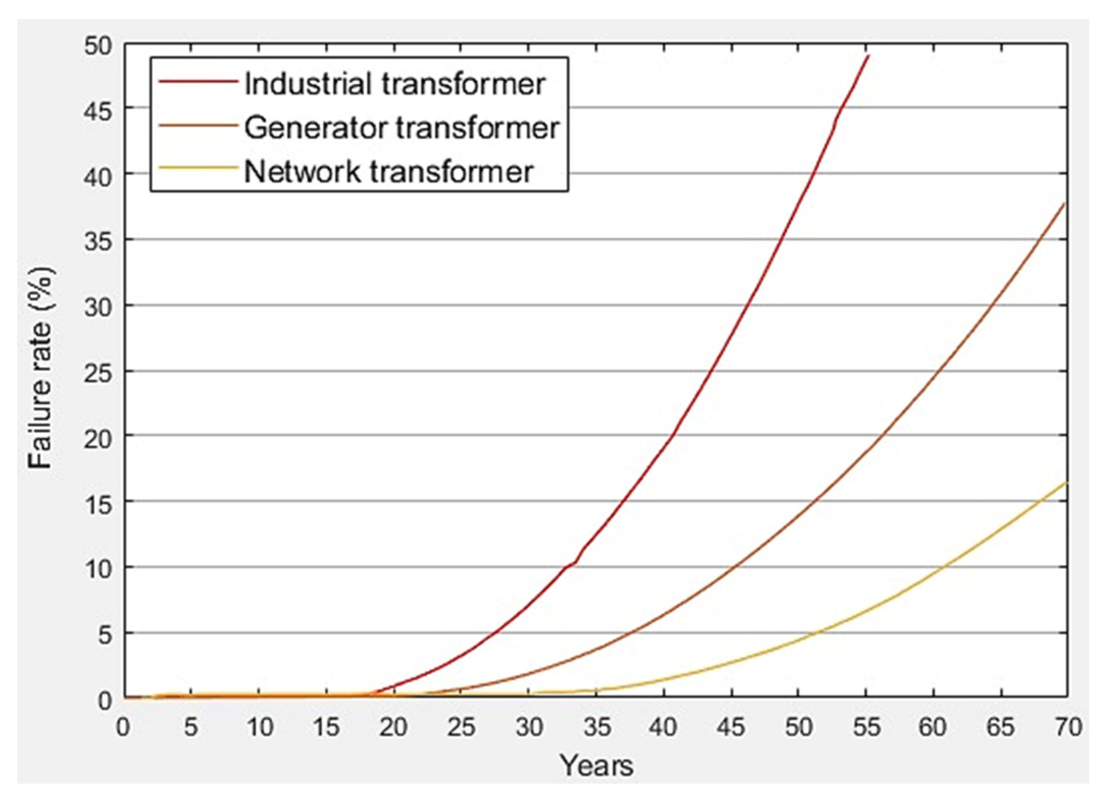
- The average age of installed LPTs in the United States and Europe is over 20 years [4]. While the life expectancy of a power transformer varies depending on how and where it is used, aging power transformers are potentially subject to an increased risk of failure. Figure 1 shows how age increases the transformer failures rate when installed in industrial plants, generation plants, and transmission networks. The failure rate curves are sharper for industrial and generator transformers because the transformers in these installations tend to be exploited more intensively.
2. Oil-Immersed Large Power Transformers: Abnormal Operating Conditions
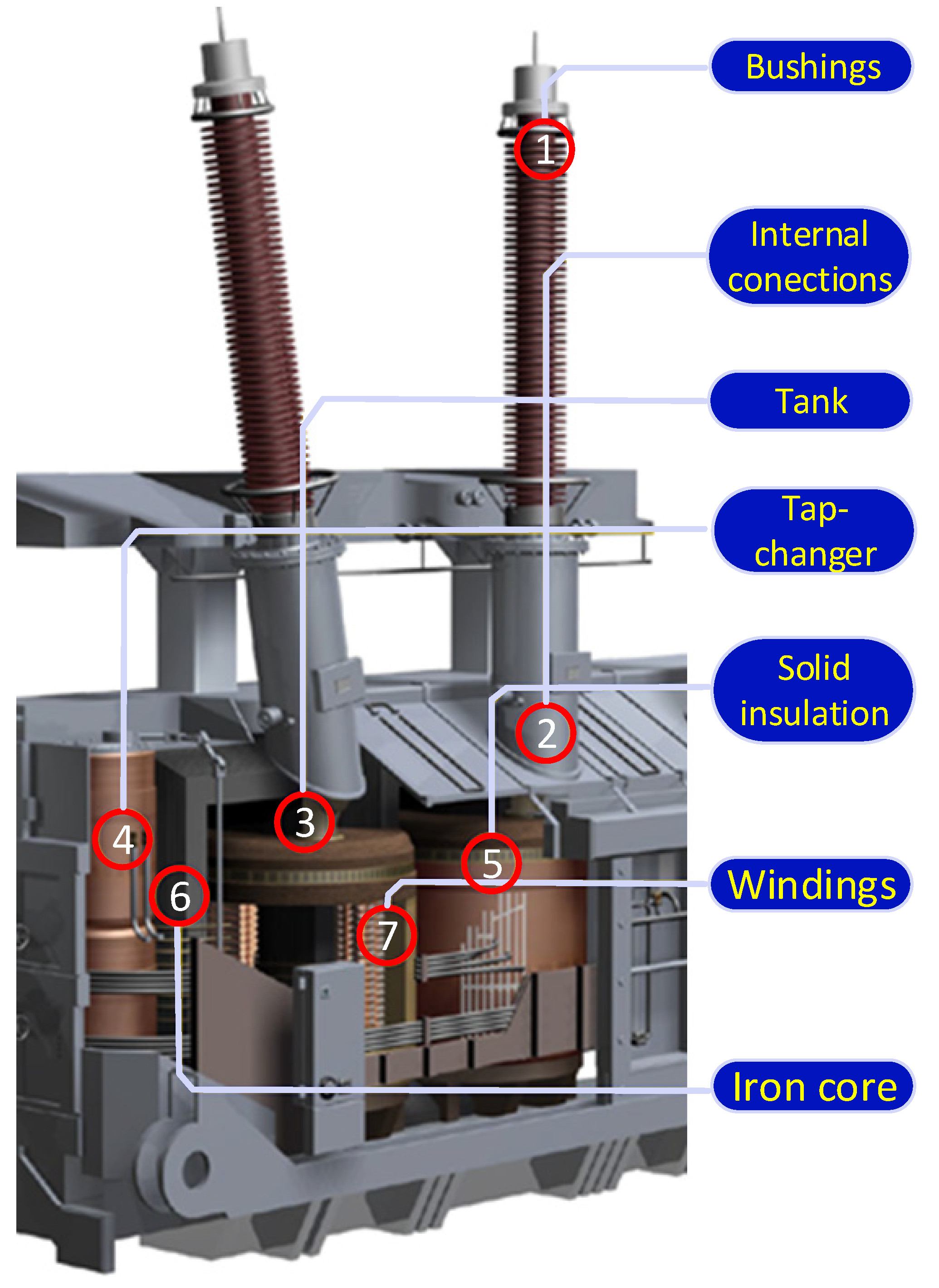
2.1. Active Part
2.1.1. Windings
2.1.2. Transformer Core
2.2. Insulation System
2.2.1. Solid Insulation
2.2.2. Liquid Insulation
2.3. Components and Accessories
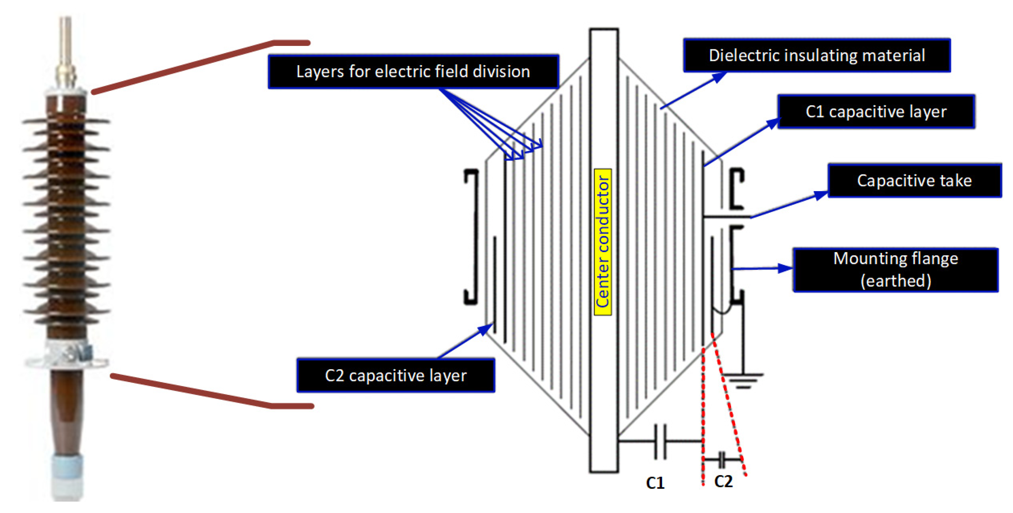
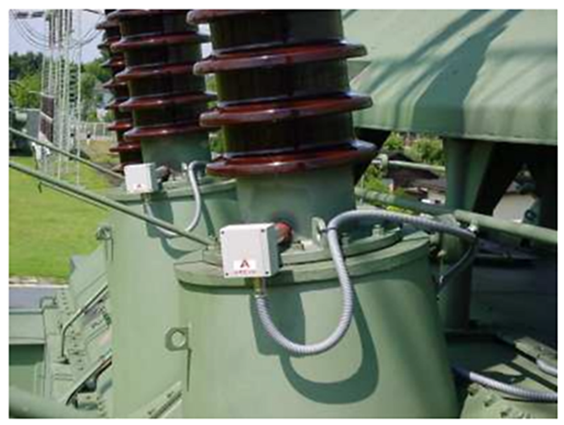
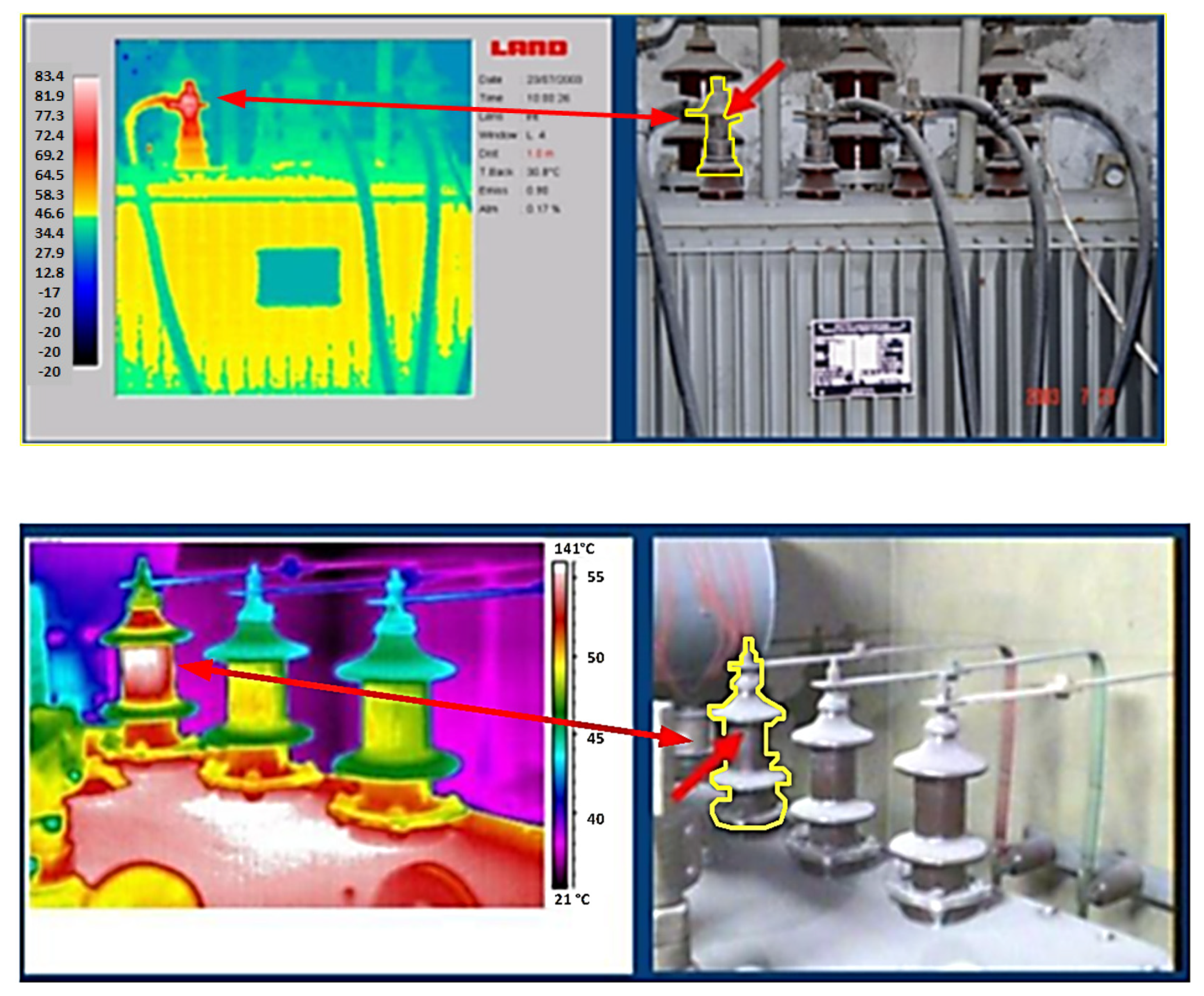
2.3.1. Bushings
- Contamination of insulators, due to deposition of contaminants (water, dust) on the surface of bushings [27] and, for highly polluted places, they must be washed regularly;

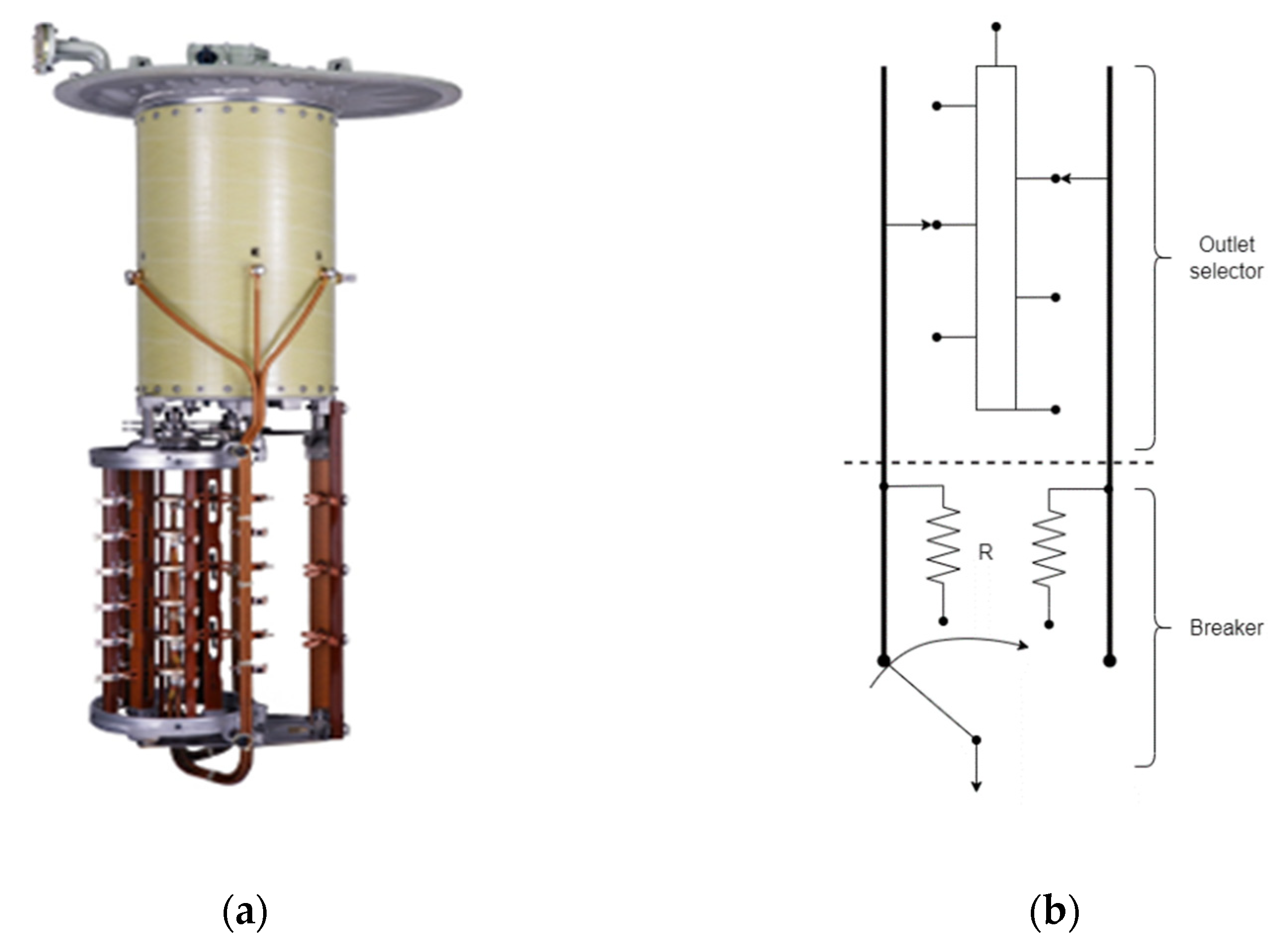
2.3.2. Tap-Changer
- Old or burnt condensers in the induction motor can lead to a loss of control in the direction of governor movement or even cause the governor motor to stop and make it impossible to change the number of turns ratio;
- With frequent use, commutator springs lose elasticity and may even break. In this case, it will not be possible to change the ratio of the number of turns of the regulator [36];
- The voltage regulator is frequently used, which leads to wear of the entire switching mechanism [24], especially in the contacts responsible for the transition of plugs, which are subject to electric arcs. In the on-load voltage regulator, the current interruption leads to the appearance of an electric arc, which leads to the formation of gases that are the same as those that appear in the main transformer tank due to dielectric failures. As such, if the tank is shared, false conclusions about dielectric failures and their location can result;
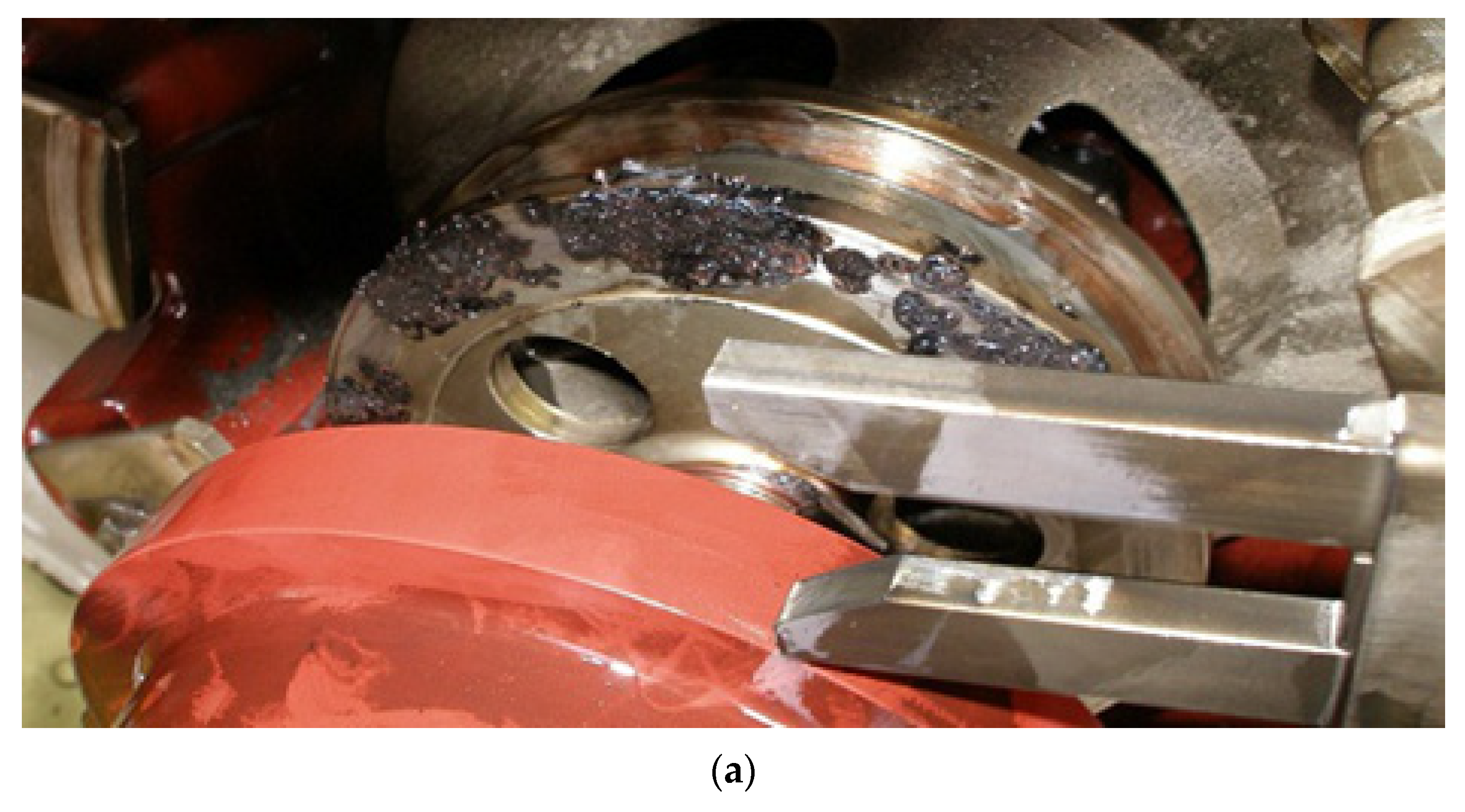
- When operating on the same contact for a long time, there is a risk of deposition of carbon particles, which can char due to the heat from the increased contact resistance. In extreme cases, as shown in Figure 10a, the contacts’ carbonization leads to the impossibility of operation as the contacts are stuck [37]. This anomaly is not very common in on-load voltage regulators and is more relevant for no-load voltage regulators.

2.3.3. Tank
2.3.4. Cooling System
3. Traditional Diagnostic Methods
3.1. Dissolved Gas-in-Oil Analysis
- R1:
- (CH4/H2)—Partial Discharges
- R2:
- (C2H2/C2H4)—Arc-electric
- R3:
- (C2H2/C2H4)
- R4:
- (C2H6/C2H2)—High-intensity discharge
- R5:
- (C2H4/C2H6)—Oil overheating > 500 °C
- R6:
- (CO2/CO)—Cellulose overheating
- R7:
- (N2/O2)—Oxygen consumption; sealing defect
3.1.1. IEC 60,599 Method
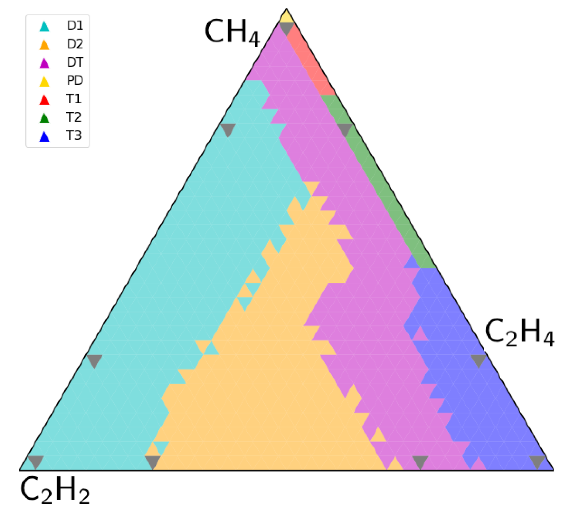
3.1.2. Duval Method
3.1.3. Key Gas Method
3.1.4. Doernenburg’s Method
3.1.5. TDCG Method (“Total Dissolved Combustible Gas”)
3.1.6. CO2/CO Ratio
3.1.7. Rogers Method
3.2. Oil Quality
3.2.1. Color
3.2.2. Interfacial Tension
3.2.3. Dielectric Breakdown Voltage
3.2.4. Dissipation Factor
3.2.5. Neutralizing Number
3.2.6. Water Content
3.2.7. Limits
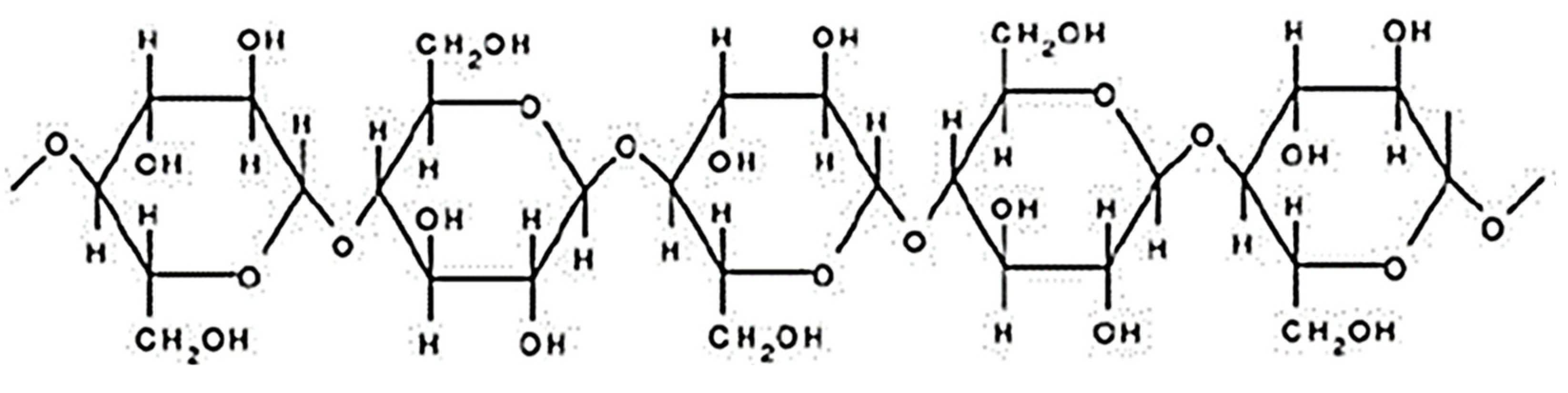
3.3. Degree of Polymerization
- and correspond to the at time t and start, respectively.
- —constant that depends on the chemical environment.
- —activation energy of the reaction in kJ/mol
- —perfect gas constant (8314 J/mol/K)
- —the absolute temperature in K
- —speed constant (aging)
3.3.1. Analysis of Furanic Compounds
- (a)
- 2-furfuraldehyde (2FAL)
- (b)
- 2-acetylfuran(2ACF)
- (c)
- 2-furfuryl alcohol (2FOL)
- (d)
- 5-methyl-2-furfuraldehyde (5MEF)
- (e)
- 5-hydroxy-methyl-2-furfuraldehyde (5HMF)
3.3.2. Direct Measurement through Paper Samples
3.4. Frequency Response Analysis
3.5. Power Factor
3.6. Excitation Current
3.7. Leakage Reactance
3.8. Electrical Insulation Resistance
3.9. Electrical Resistance of Windings
3.10. Partial Electrical Discharges
3.11. Relationship between Turns
3.12. Return Voltage and Polarization Currents
3.13. Mechanical Vibrations
3.14. Temperature
3.15. Infra-Red Test
3.16. Bushings Condition
3.17. Tap-Changer Condition
4. Online Diagnostic Models for Power Transformers
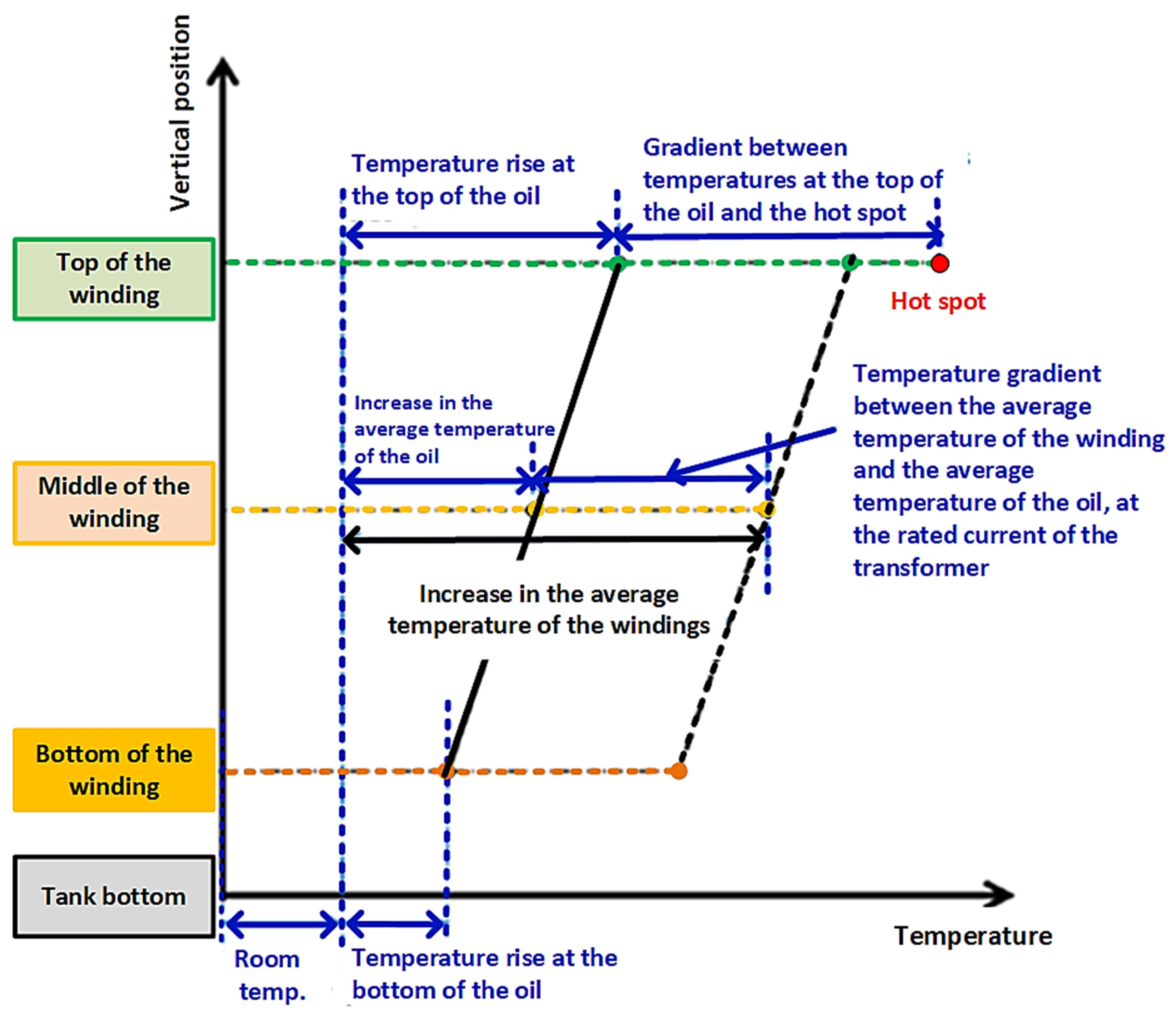
4.1. Thermal Model
- The oil temperature in the transformer tank increases linearly between the bottom and the top, regardless of the type of cooling;
- The temperature along the winding also increases linearly between the bottom and the top, regardless of the type of cooling. For the same horizontal position, this temperature always exceeds that of the oil by the value of a constant gr (gradient between the average temperature of the windings and the oil);
- The temperature rise of the hot spot is greater than the temperature rise of the winding on top of the winding. The difference is determined by multiplying the constant gr by the hot spot factor (HSF).
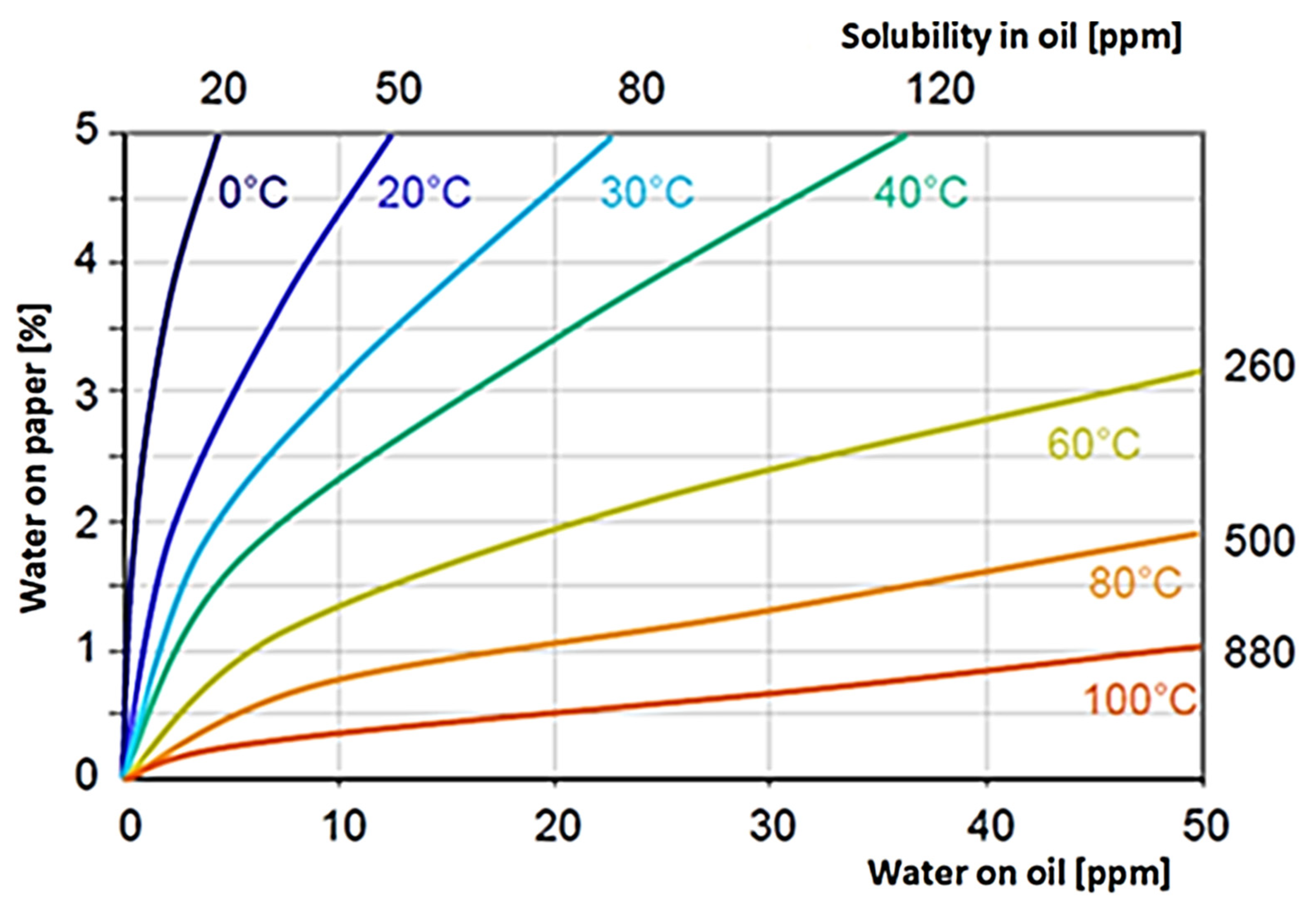
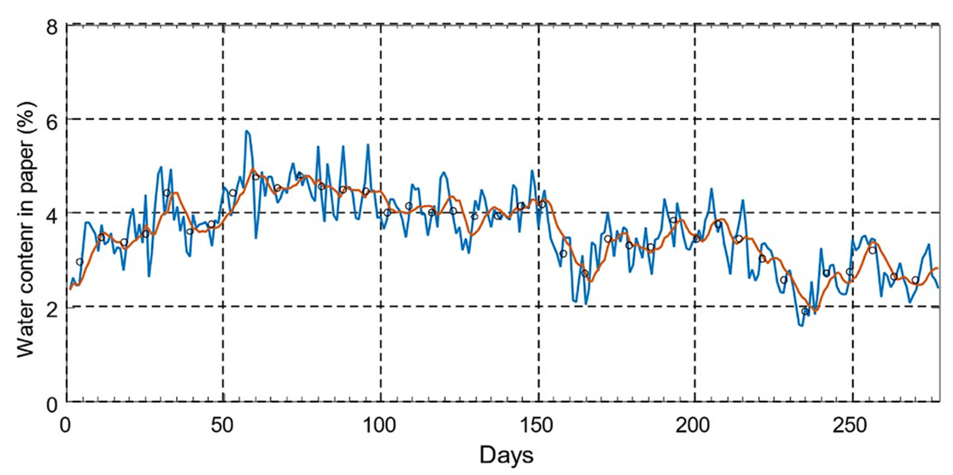
4.2. Model for Estimating Water Content in Insulation (Paper and Card) and Temperature of Water Bubbles
- Residual water that comes from manufacturing—During manufacturing, water is installed in the different components of the transformer and, despite drying, there is always a portion of water that remains, typically 0.4–1%;
- Entry from the atmosphere—The atmosphere is considered the main source of water for transformers, which can enter, for example, by exposure to humid air during installation or repairs and due to cracks that expose the inside of the transformer;
- Aging of oil and cellulose—The decomposition of cellulose, which essentially consists of breaking the bonds of glucose chains, is reflected in the appearance of water and other compounds. Oil oxidation also contributes to water formation. The normal annual water increase is approximately 0.1% [54].
4.2.1. Measurement Methods
- Obtaining an oil sample from the transformer in service;
- Measurement of water content in oil (ppm) through Karl Fischer titration;
4.2.2. Calculation of Water Content in the Paper
4.2.3. Temperatures Considered in the Previous Equations
4.2.4. Limits and Definitions
- <69 kV, 3% maximum
- 69 kV–230 kV, 2% maximum
- >230 kV, 1.25% maximum
- Dry insulation, 0–2%
- Wet insulation, 2–4%
- Very wet insulation, >4.5%
4.2.5. Temperature for Water Bubbles Occurring
4.3. Transformer Aging Model
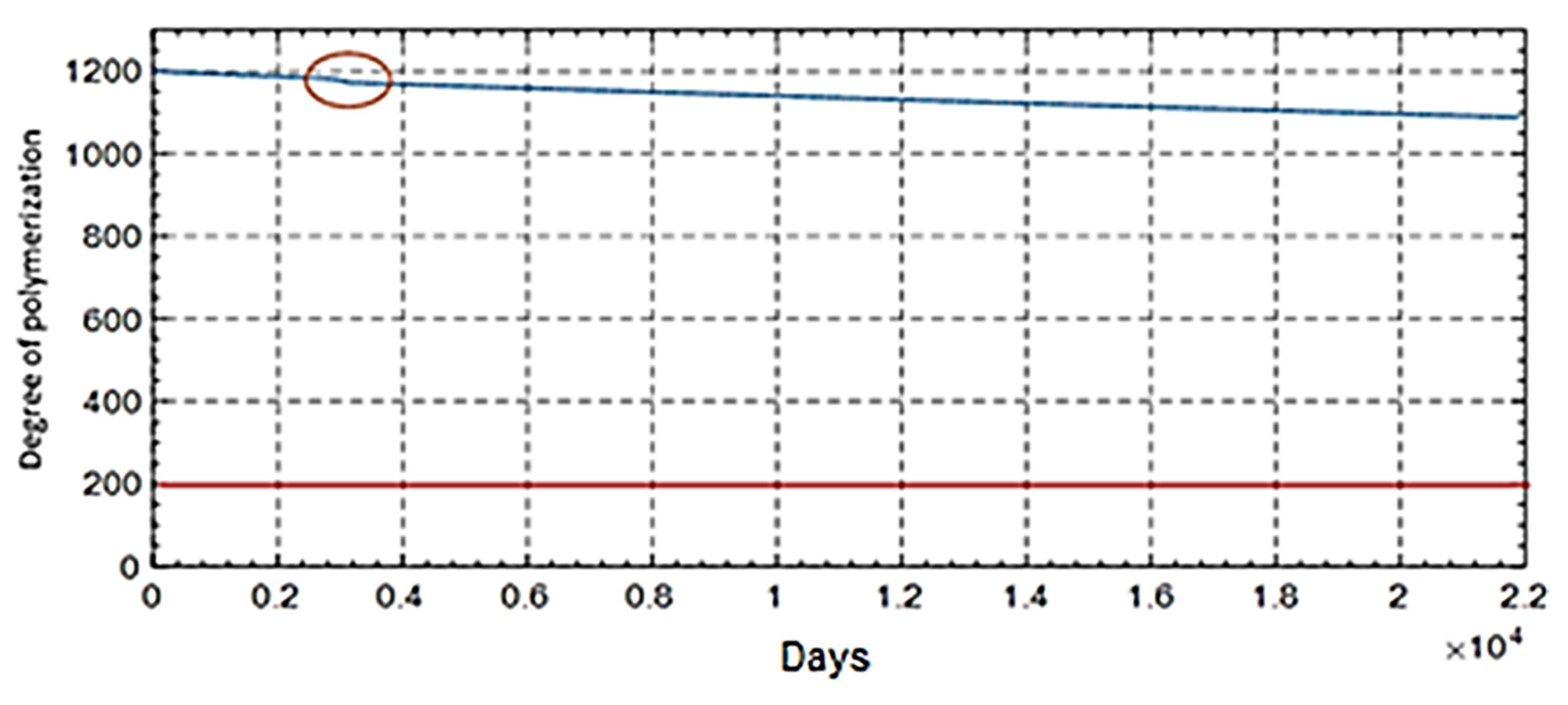
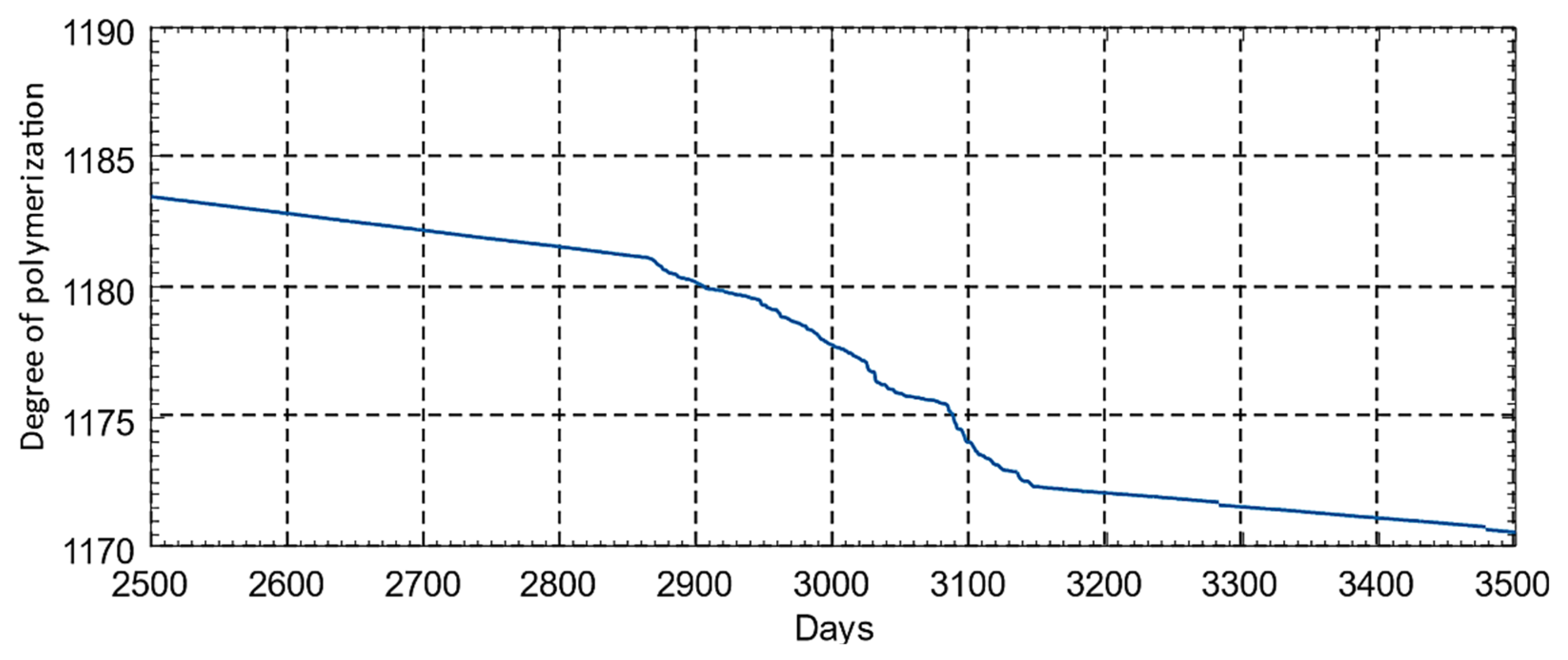
4.3.1. Kraft Paper
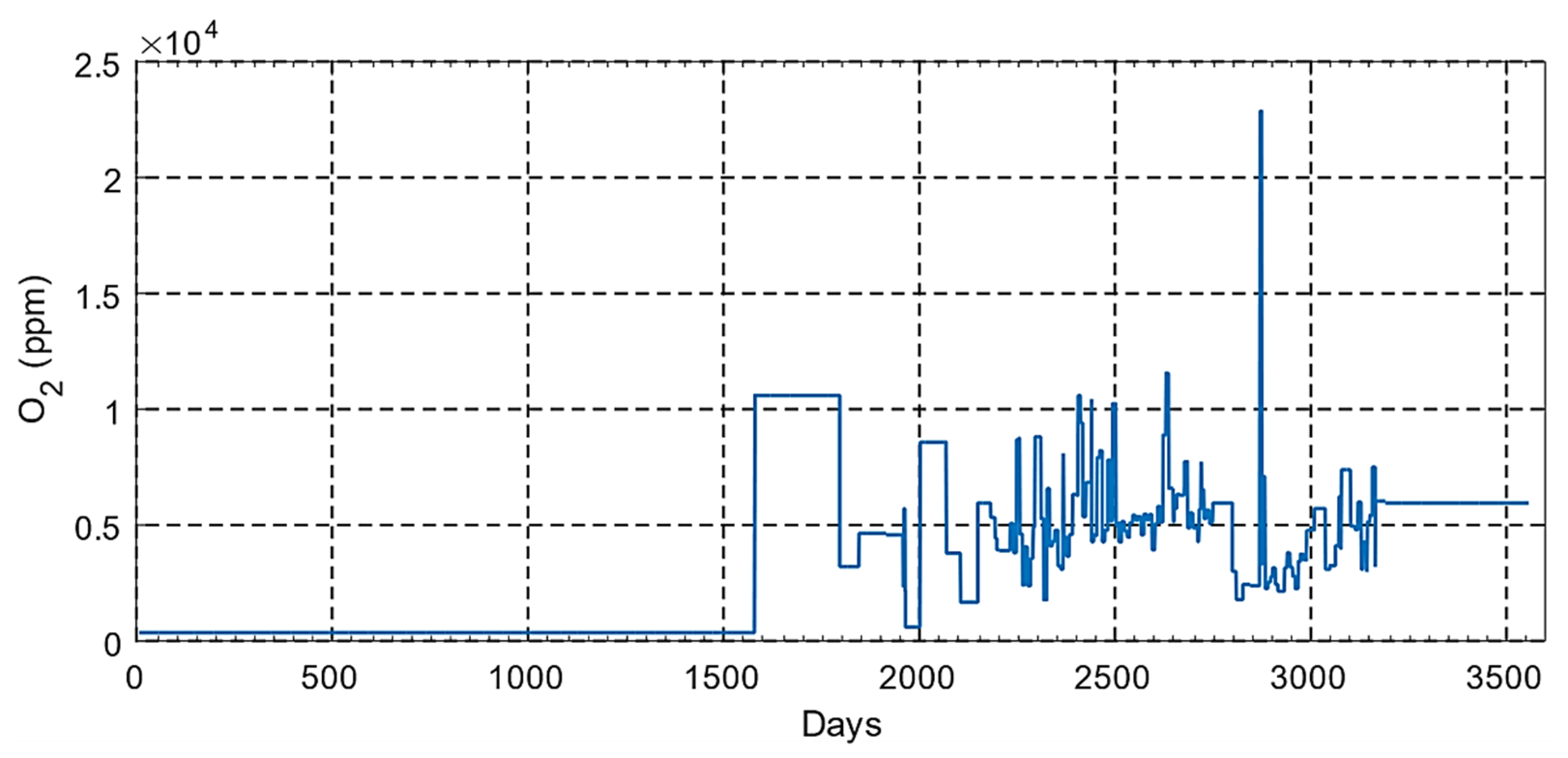
- Low oxygen content in oil (O2 < 6000 ppm):
- Average oxygen content in the oil (7000 ppm < O2 < 14,000 ppm):
- High oxygen content in oil (16,500 ppm < O2 < 25,000 ppm):
4.3.2. Thermally Improved Kraft Paper
- Low oxygen content in oil (O2 < 6000 ppm):
- Average oxygen content in the oil (7000 ppm < O2 < 14,000 ppm):
- High oxygen content in oil (16,500 ppm < O2 < 25,000 ppm):
4.4. Load Factor Monitoring Model
4.5. Analysis Model of Gases Dissolved in Oil
4.6. Model for Monitoring and Diagnosing Crossings
4.7. Model for On-Load Voltage Regulator Monitoring and Diagnosis
4.8. Cooling System Monitoring Model
5. Case study in a 1400 MVA Three-Phase Large-Power Transformer
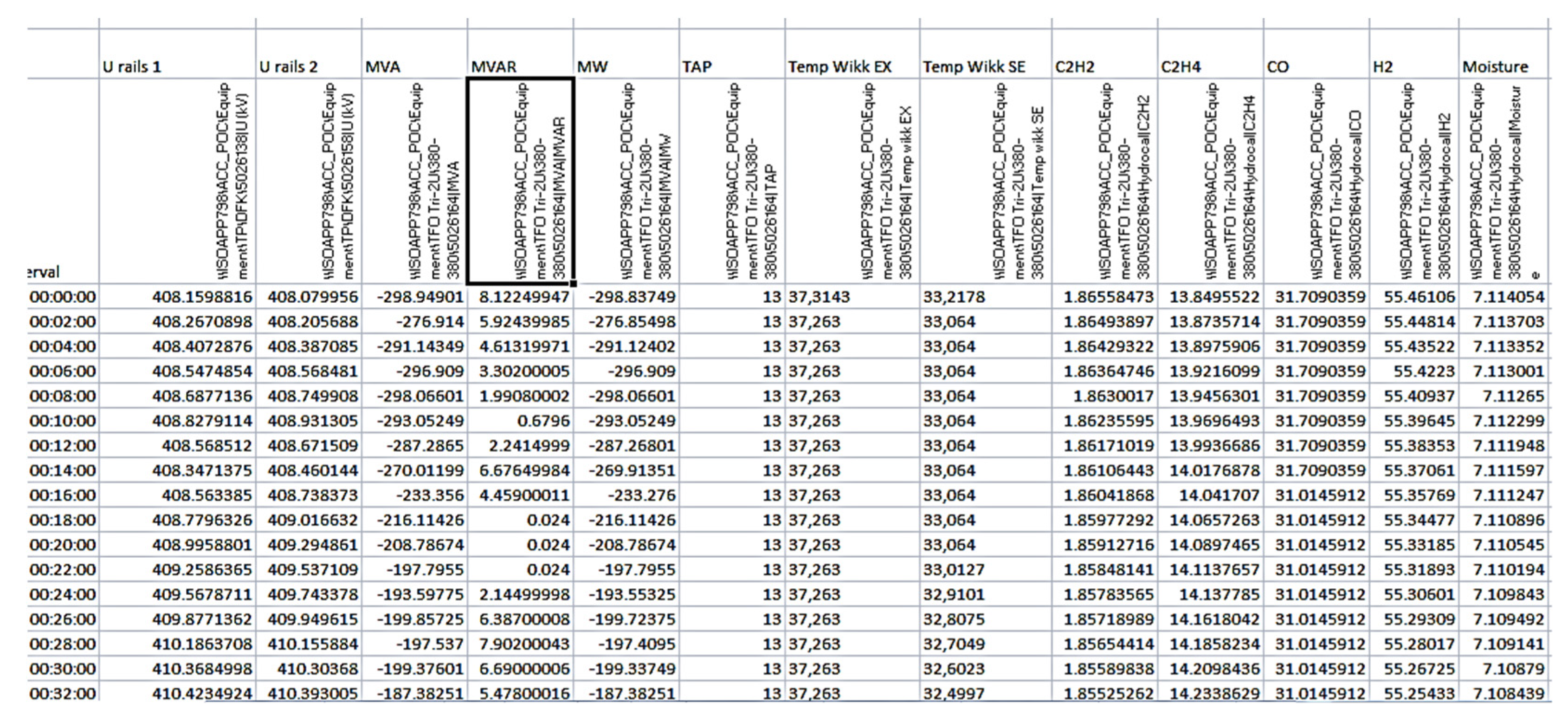
5.1. Measured Quantities
5.1.1. Online Quantities and Their Variables’ Representation
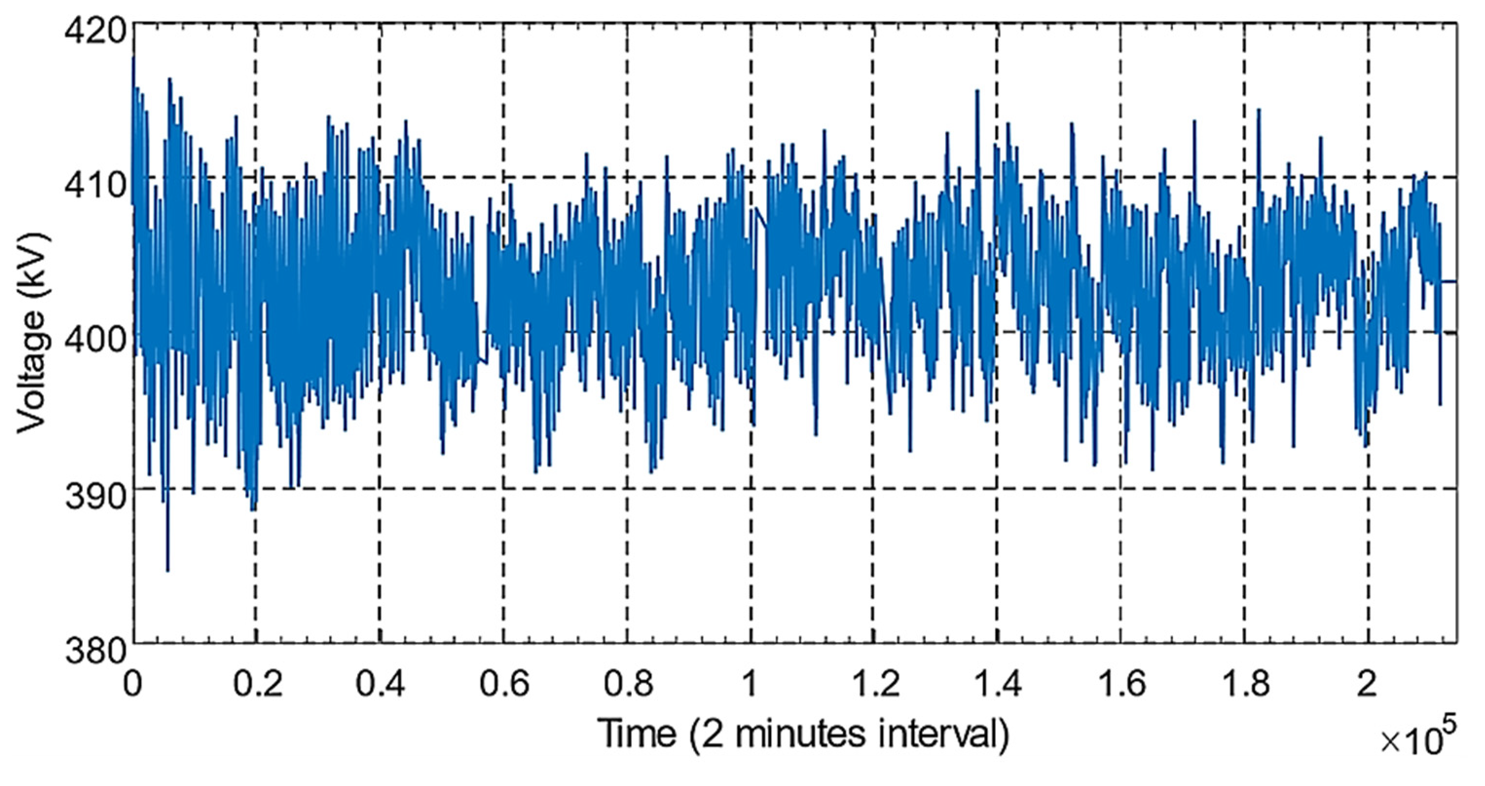
- Primary and secondary voltage (U1 and U2);
- Apparent, reactive, and active power (MVA, MVAR, and MW);
- Position of the on-load voltage regulator (TAP);
- Excitation (EX) and series (SE) unit temperatures (Temp_Windings_EX and Temp_Windings SE), and;
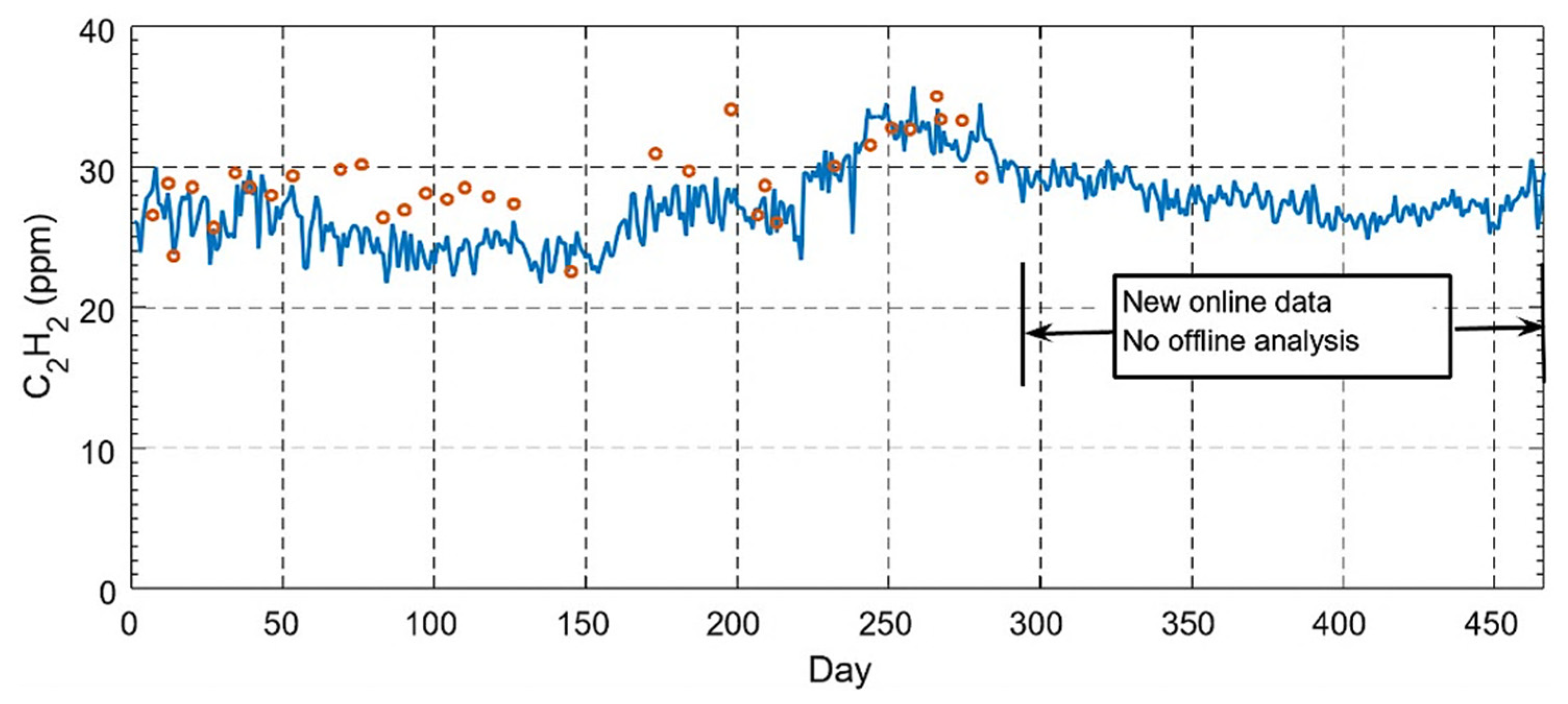
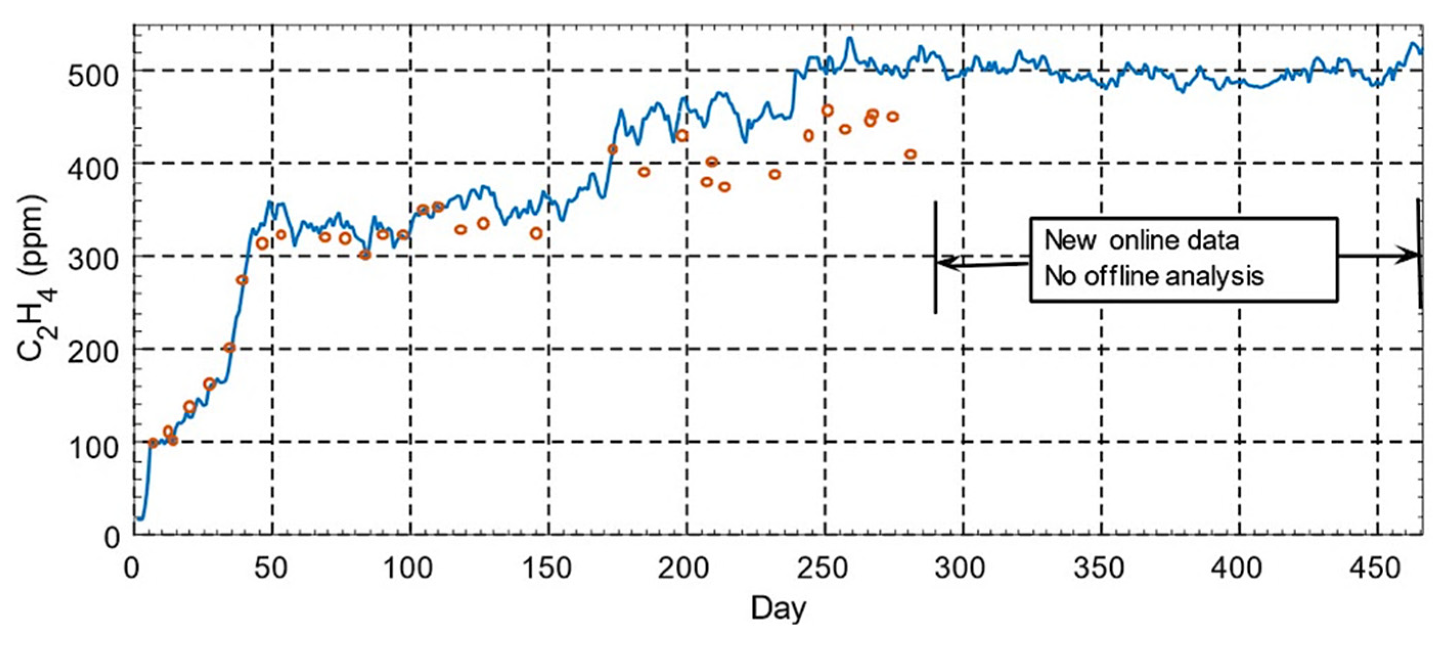
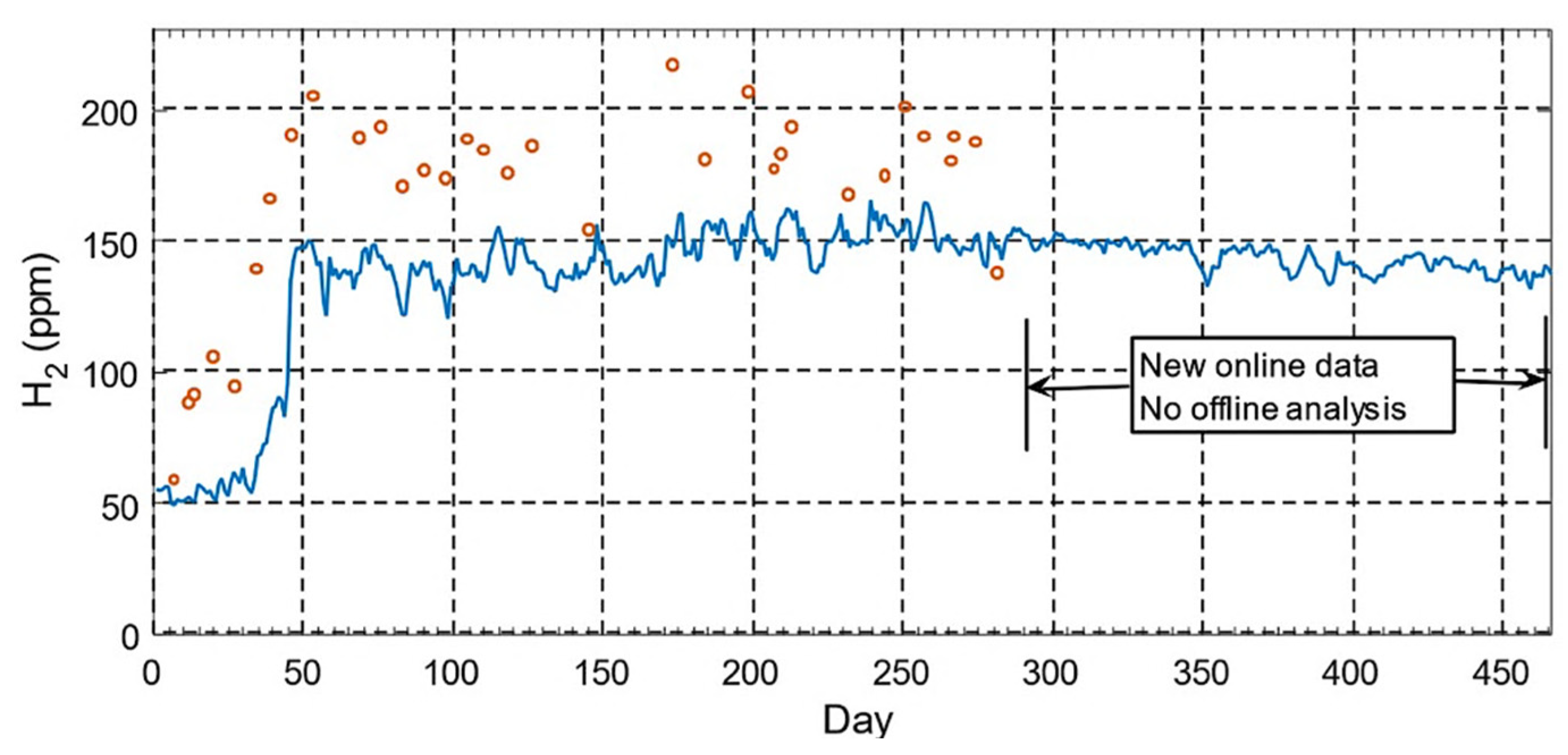
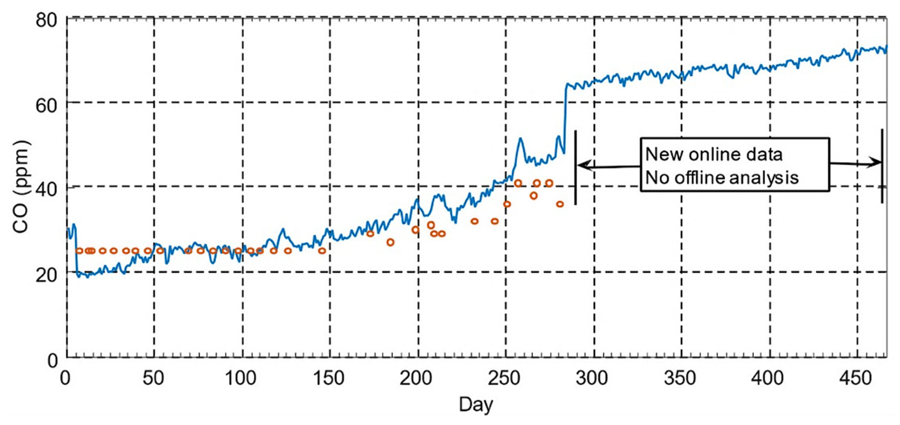
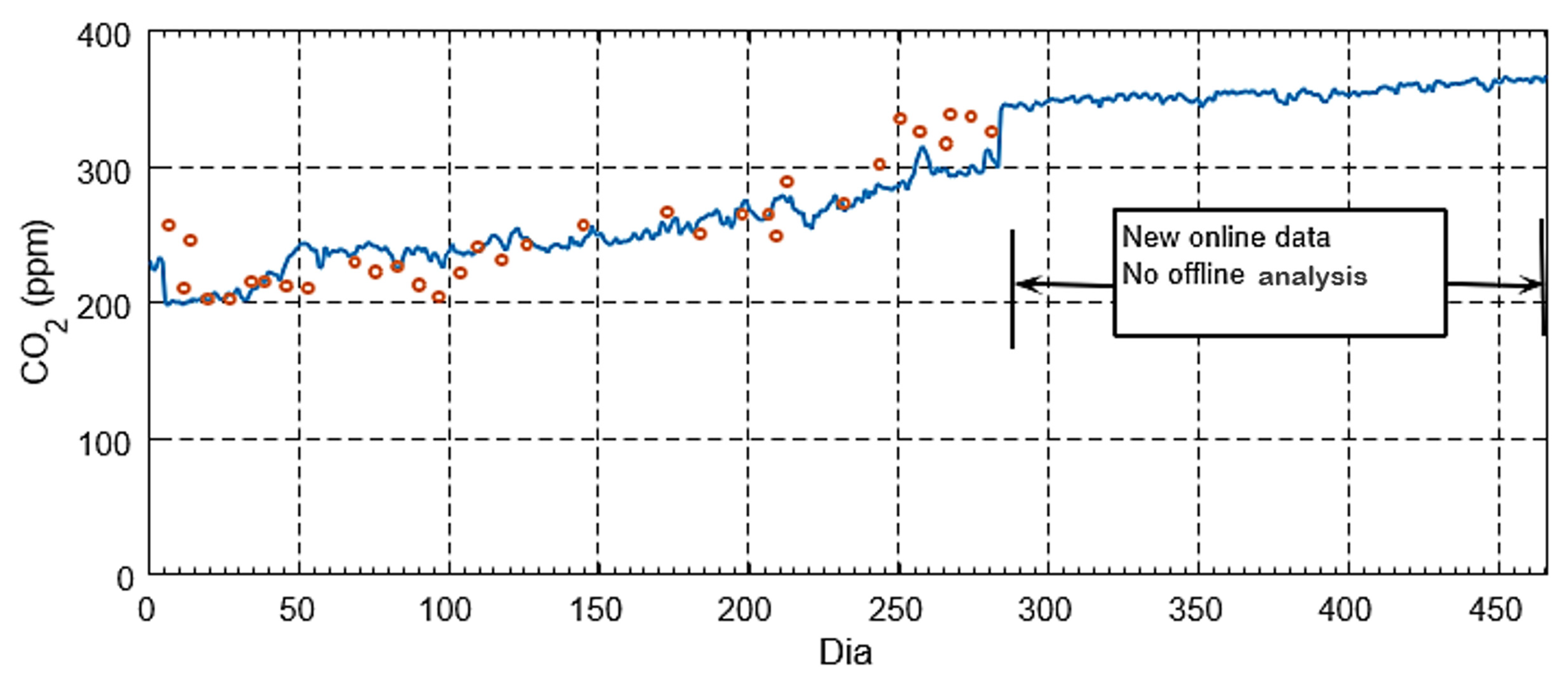
- Concentration of gases (C2H2, C2H4, H2, and CO) and water in oil, in ppm, measured in the excitation unit.
5.1.2. Offline Quantities and Their Variables’ Representation
- Gas concentration: H2, O2, N2, CO, CO2, CH4, C2H4, C2H6, and C2H2;
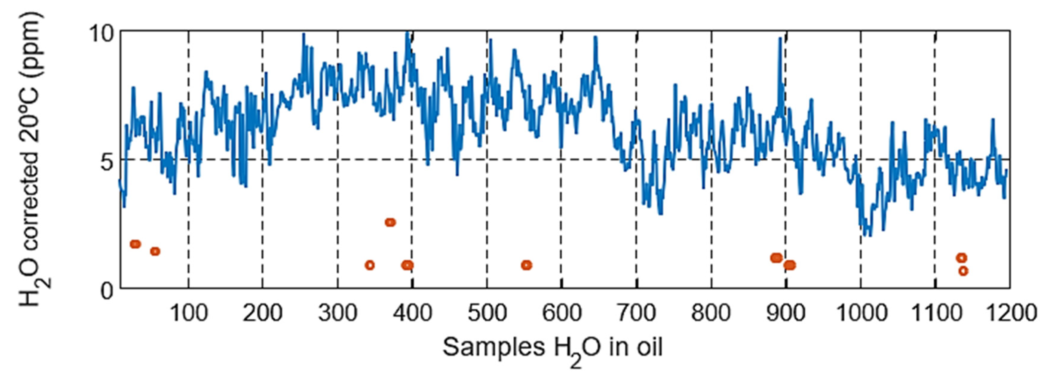
- Concentration of water in oil;
- Furans: 5-hydroxymethyl-2-furfural (5HMF), 2-furfuryl alcohol (2FOL), 2-furfural (2FAL), 2-acetyl furan (2ACF), 5-methyl-2-furfural (5MEF);
- Oil Quality (Color, Appearance, Density, Neutralizing Number, Dissipation Factor (90 °C), Disruption Voltage, Phenolic Inhibitor, Presence of Insolubles, Precipitated Substances), and;
- Oil temperature at the bottom.
5.2. Data Quality
5.2.1. Remote Sensing
5.2.2. Sampling
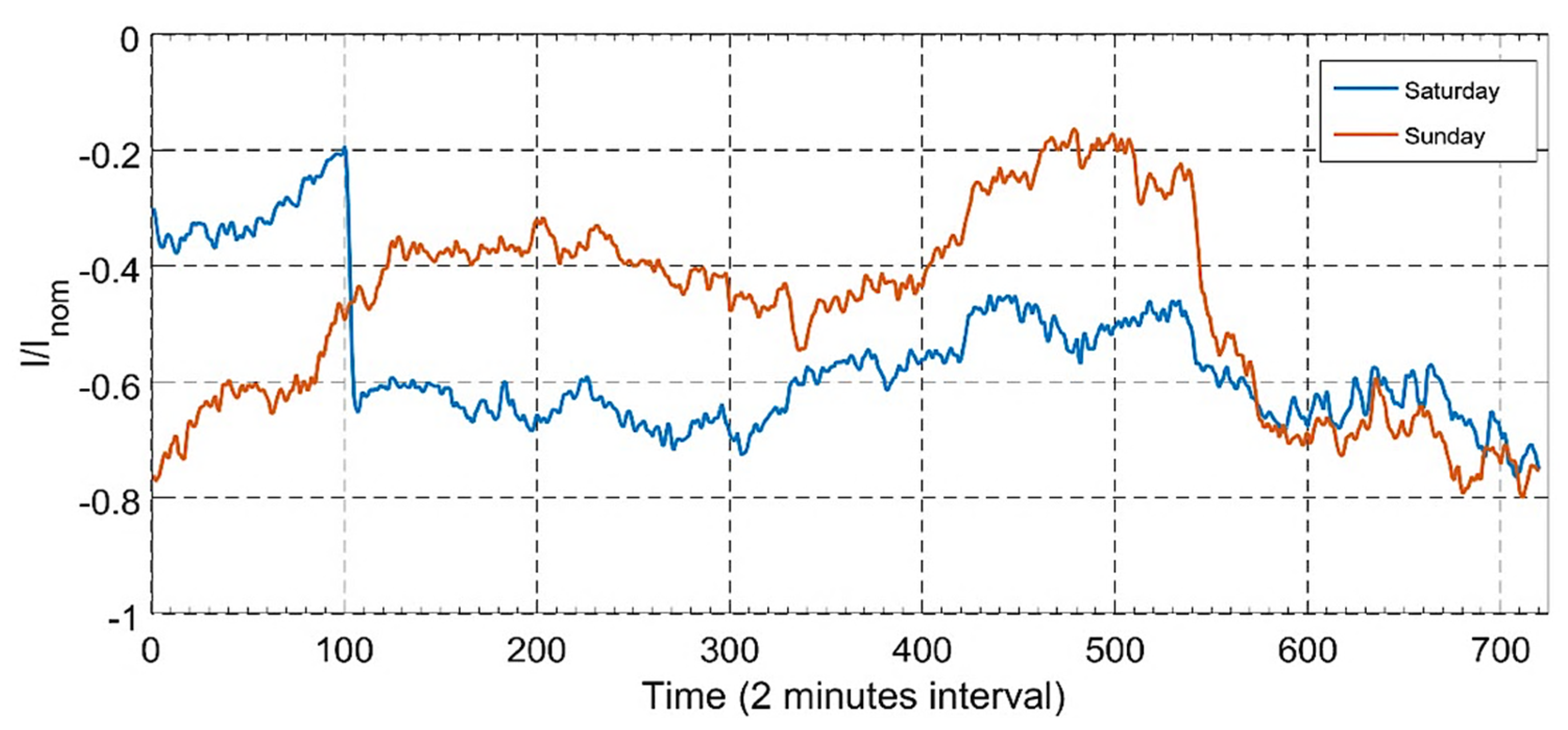
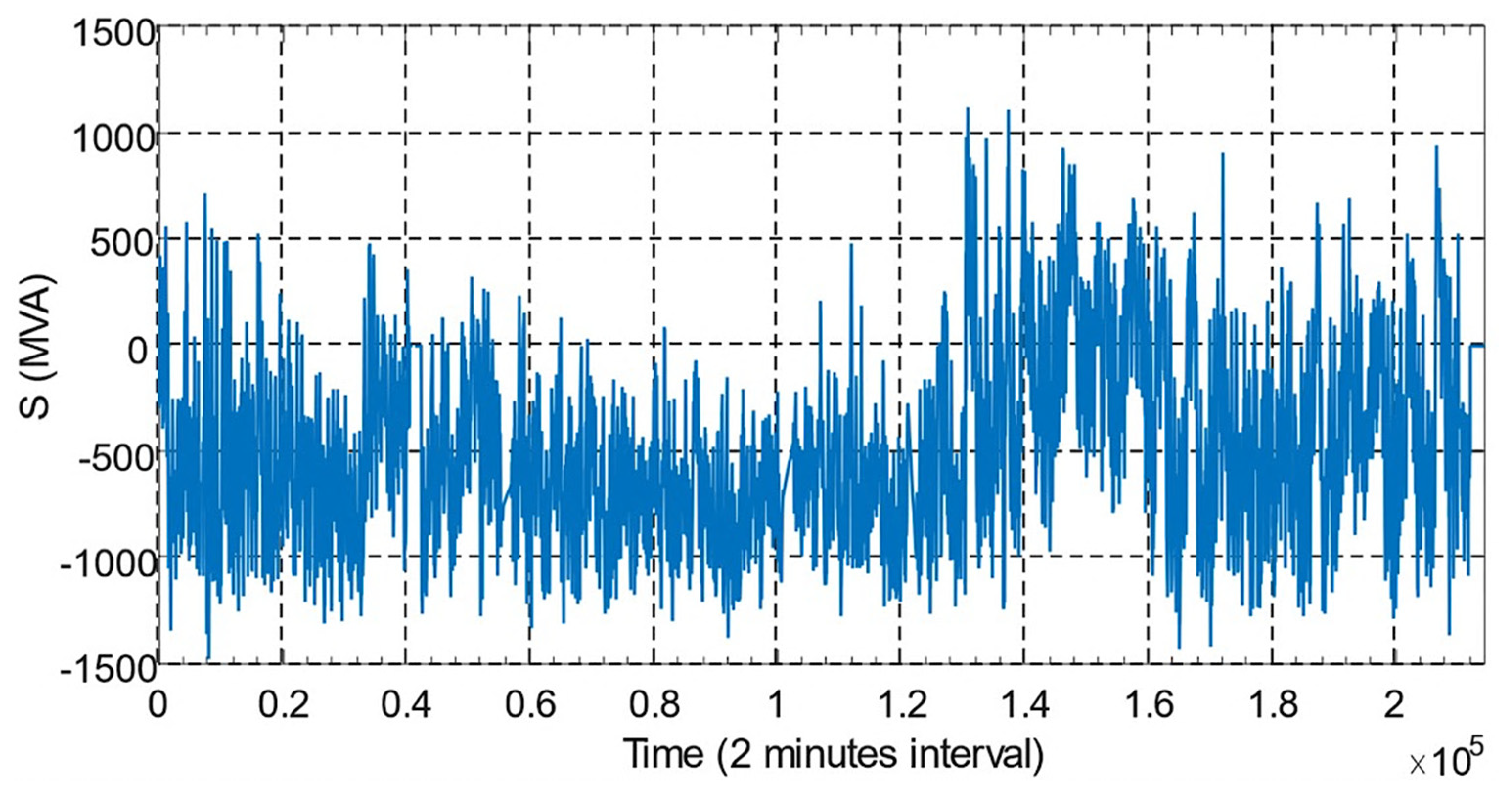
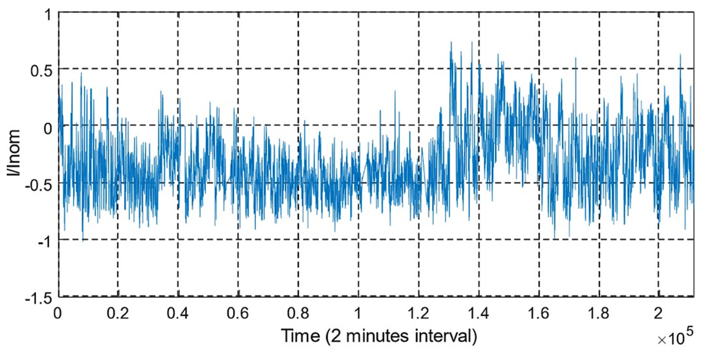
5.3. Load Factor
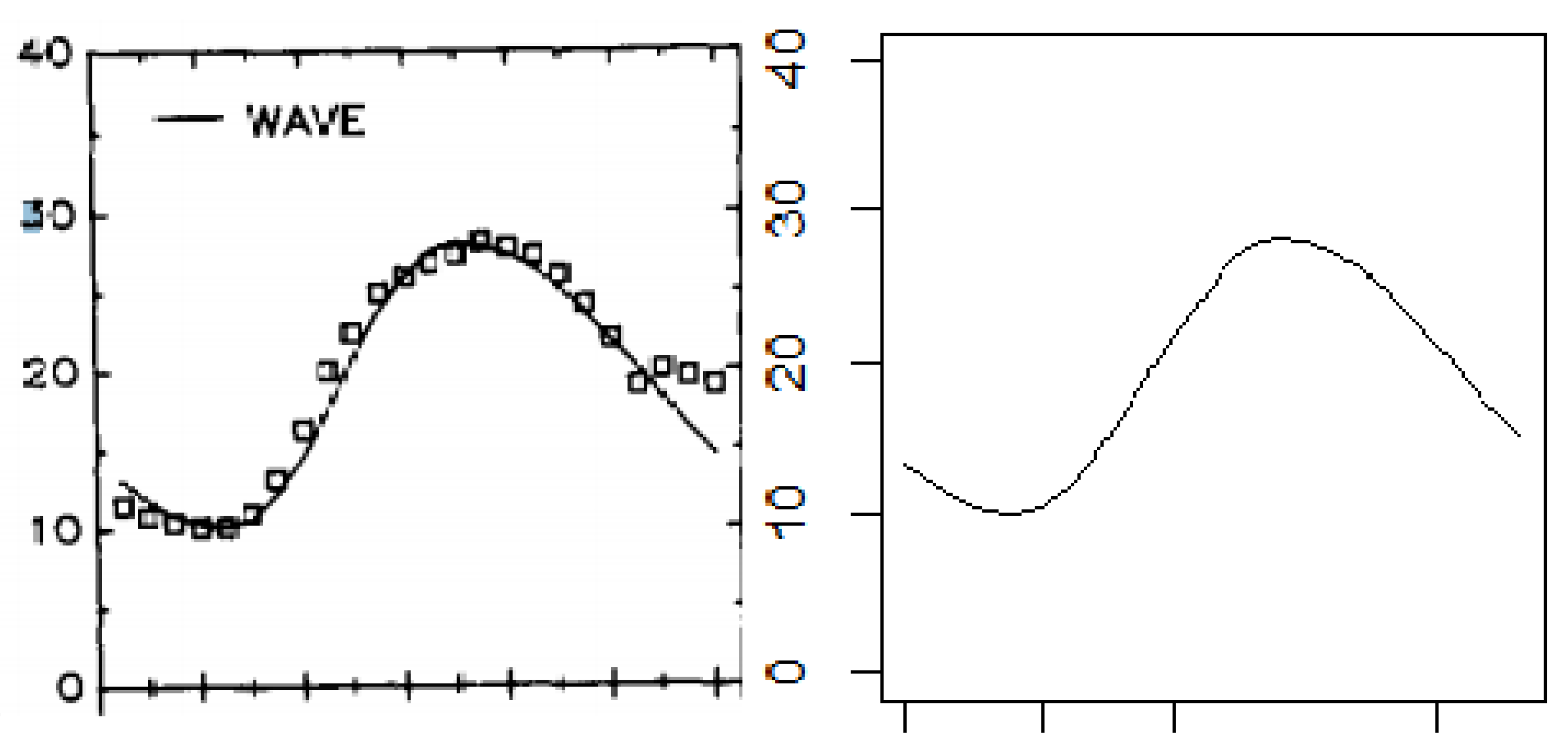
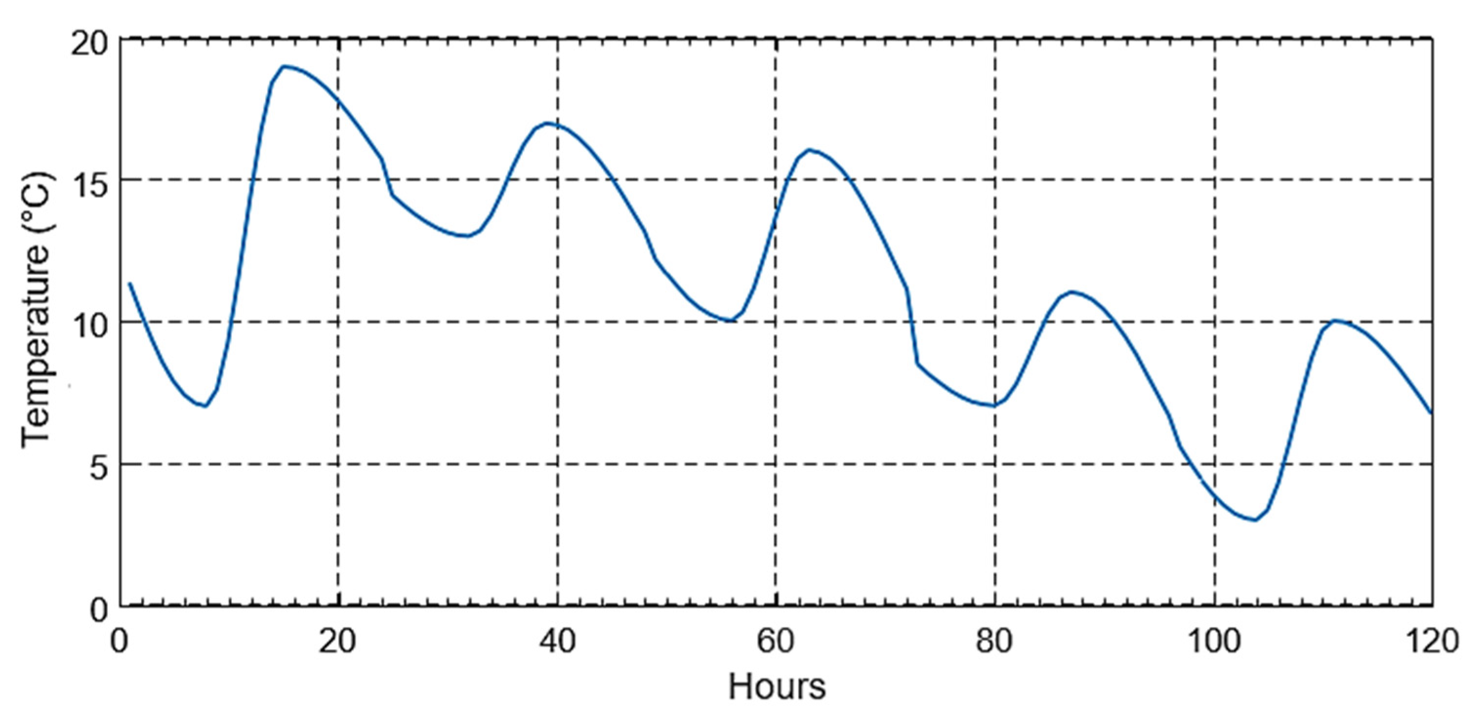
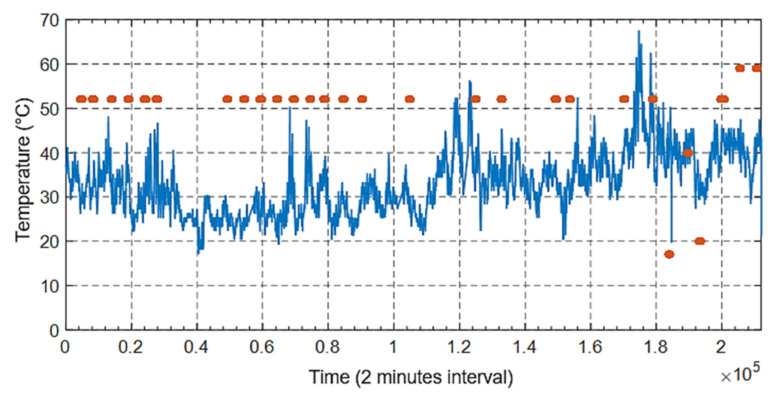
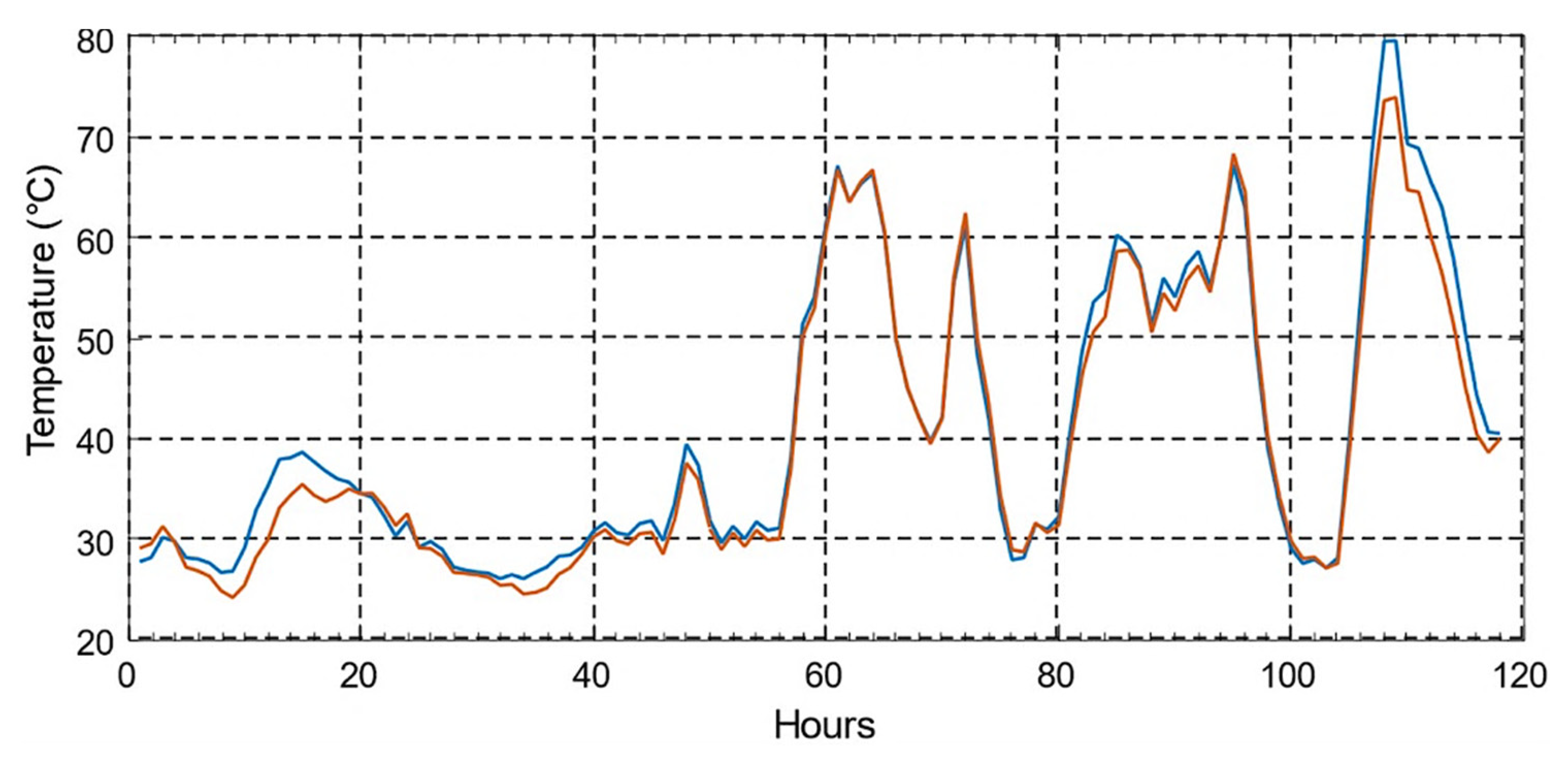
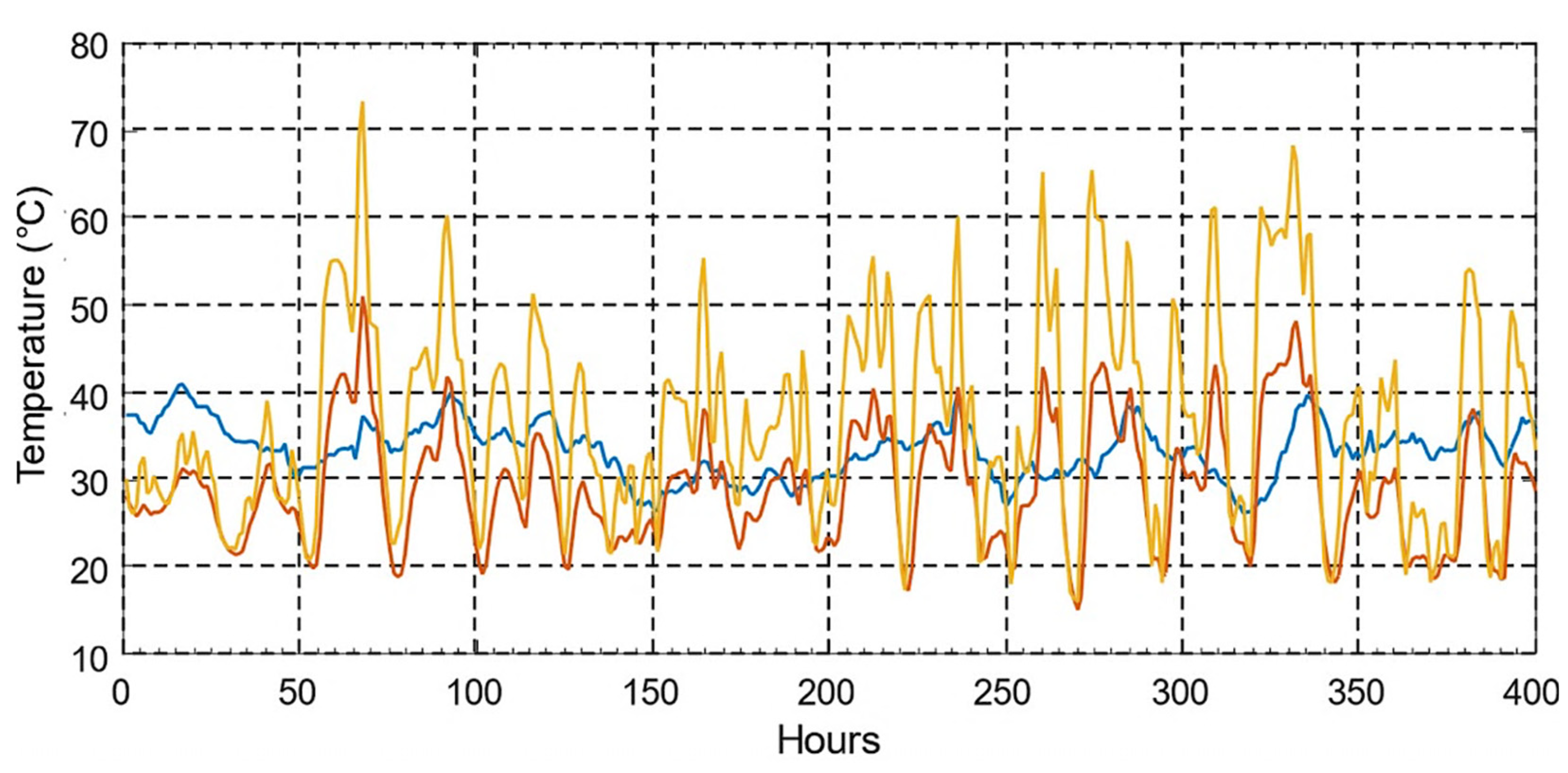
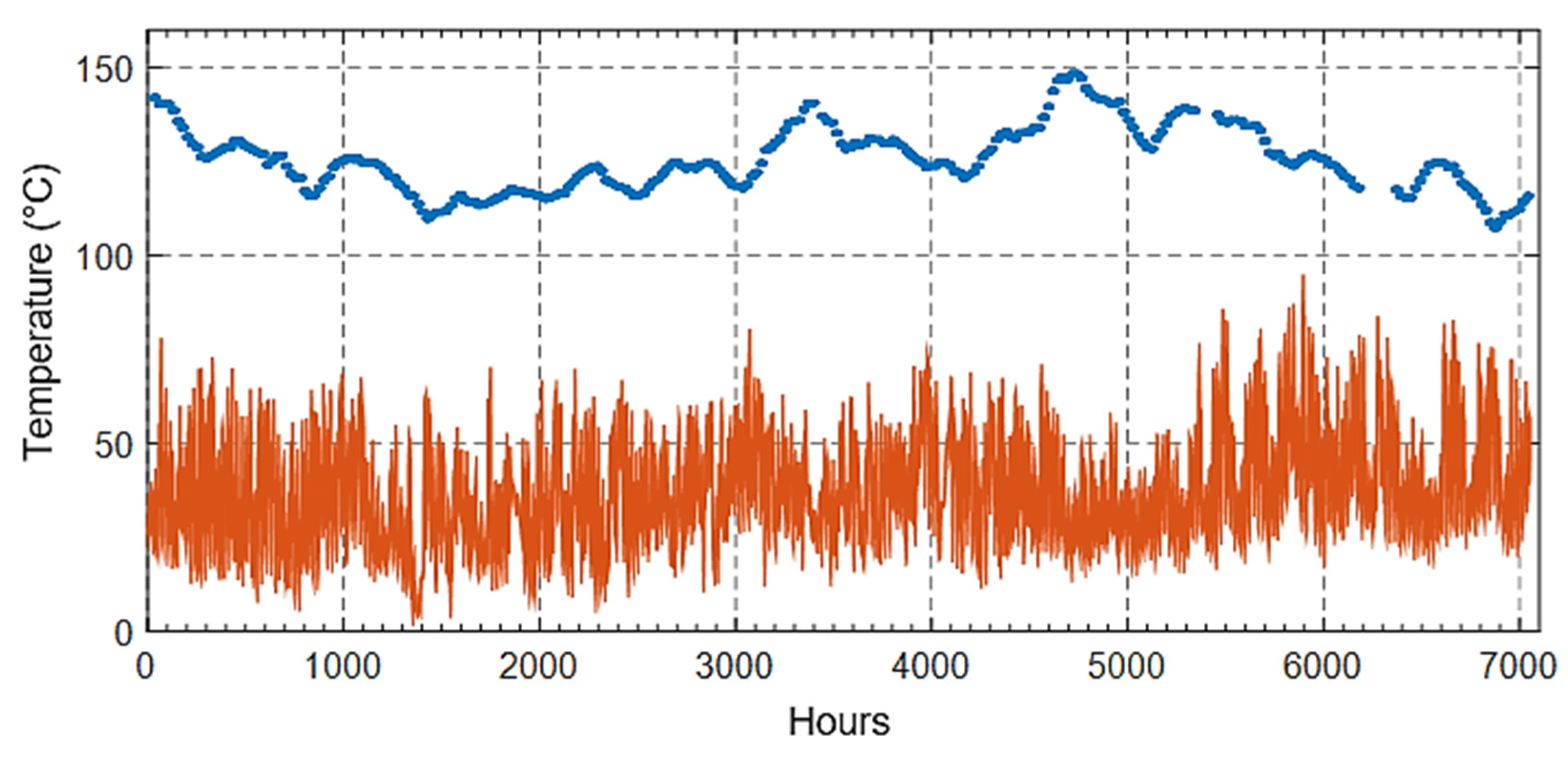
5.4. Temperature
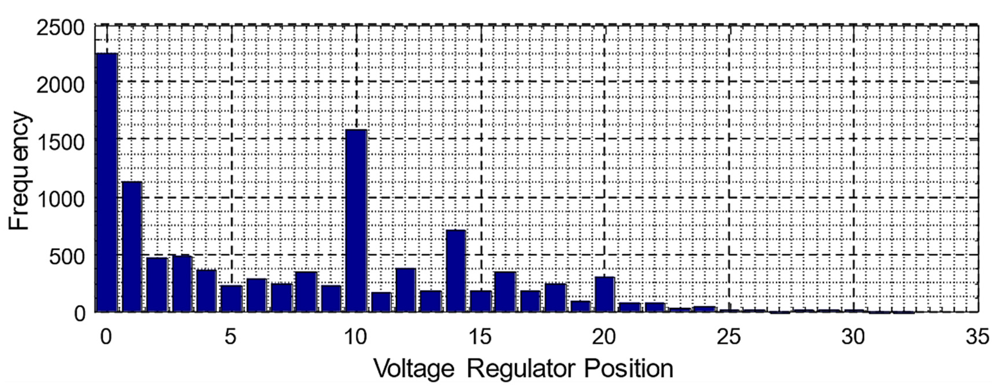
5.5. Position of the On-Load Voltage Regulator (TAP)
5.6. Dissolved Gases in Transformer Oil: Online and Offline
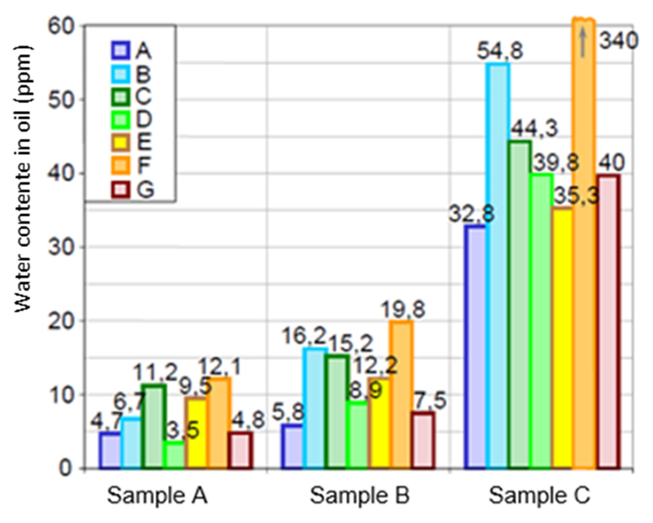
5.7. Water
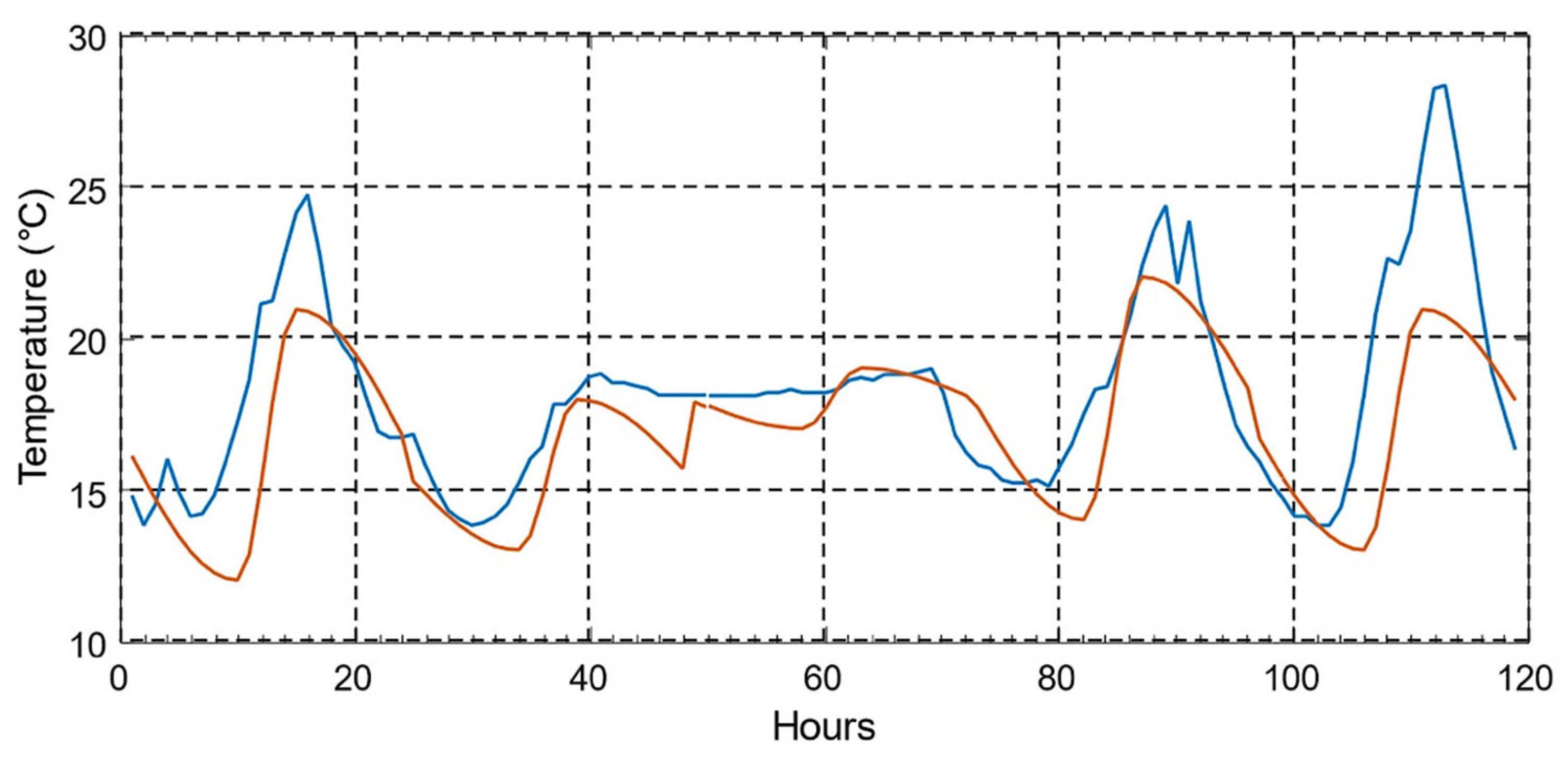
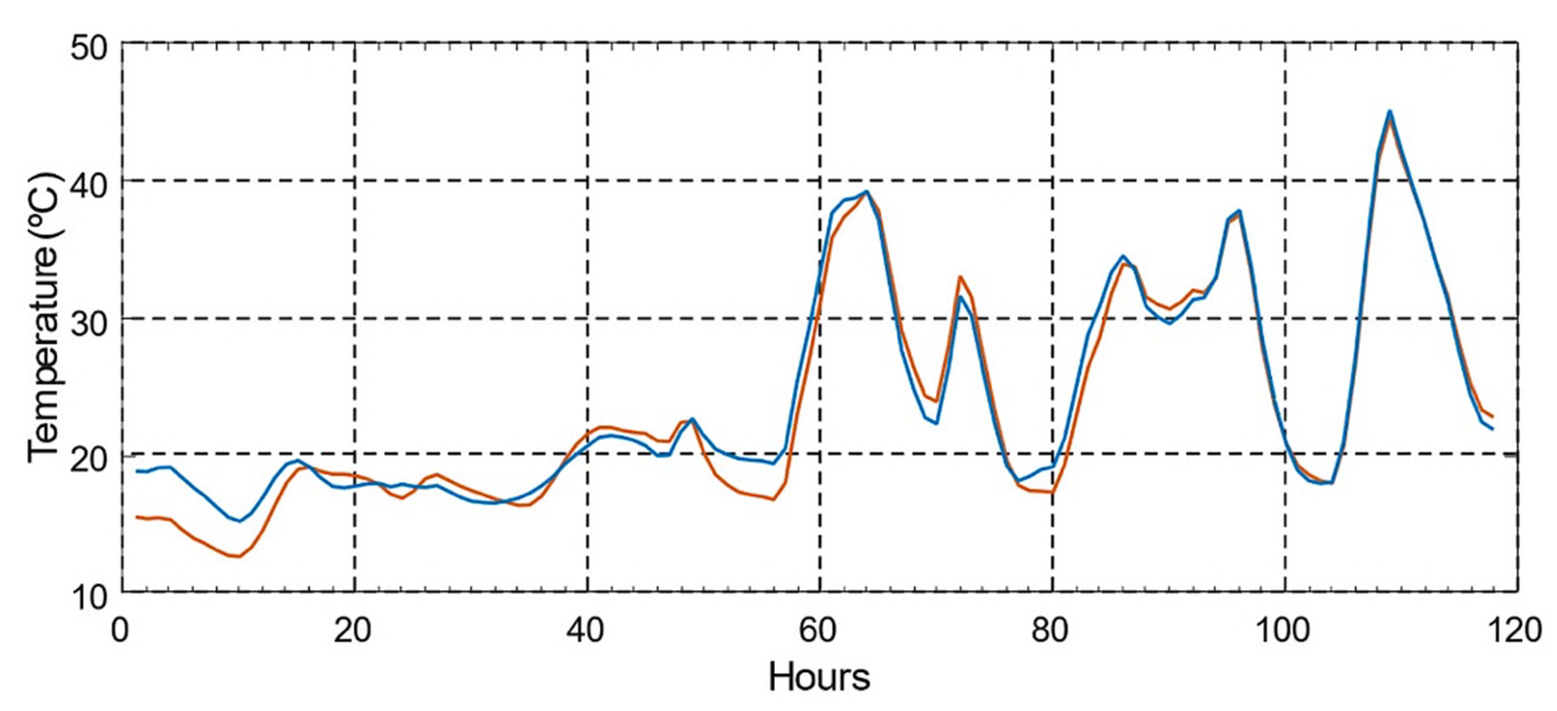
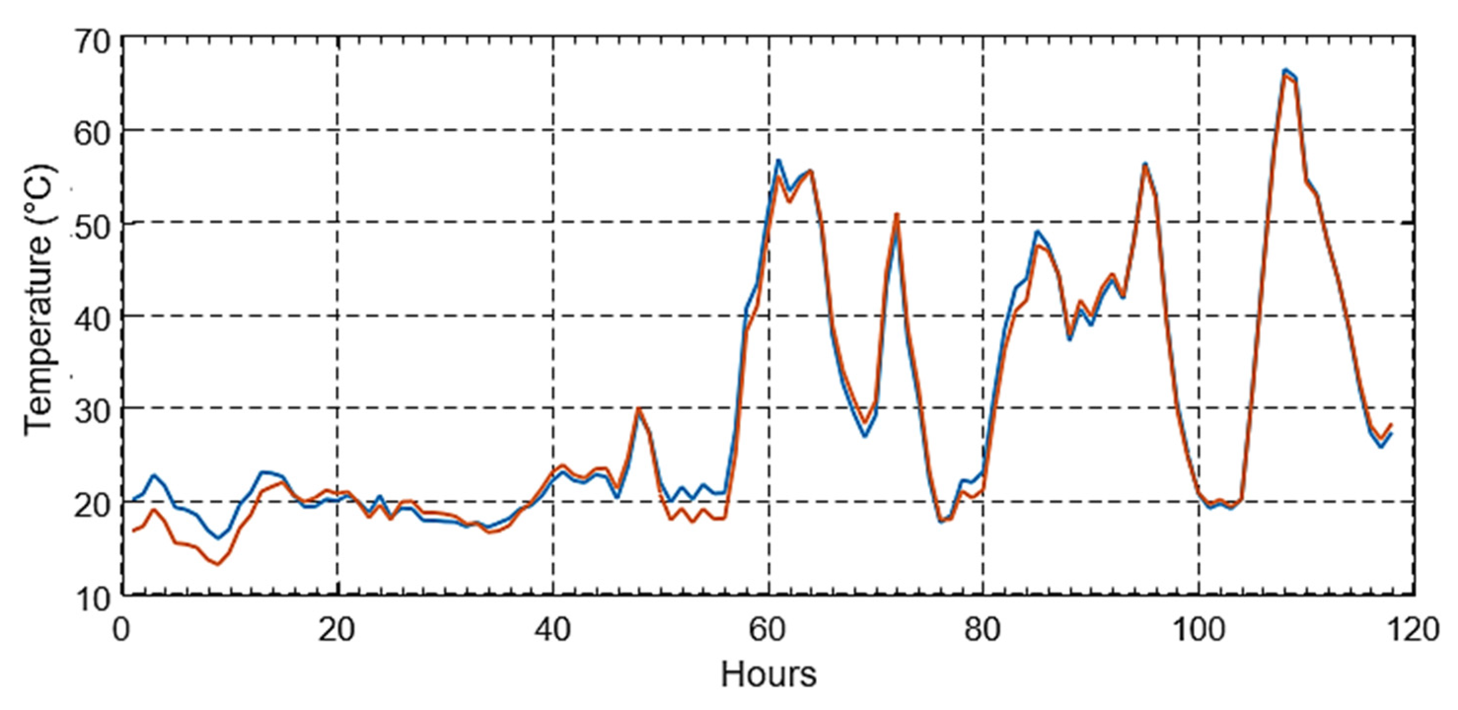
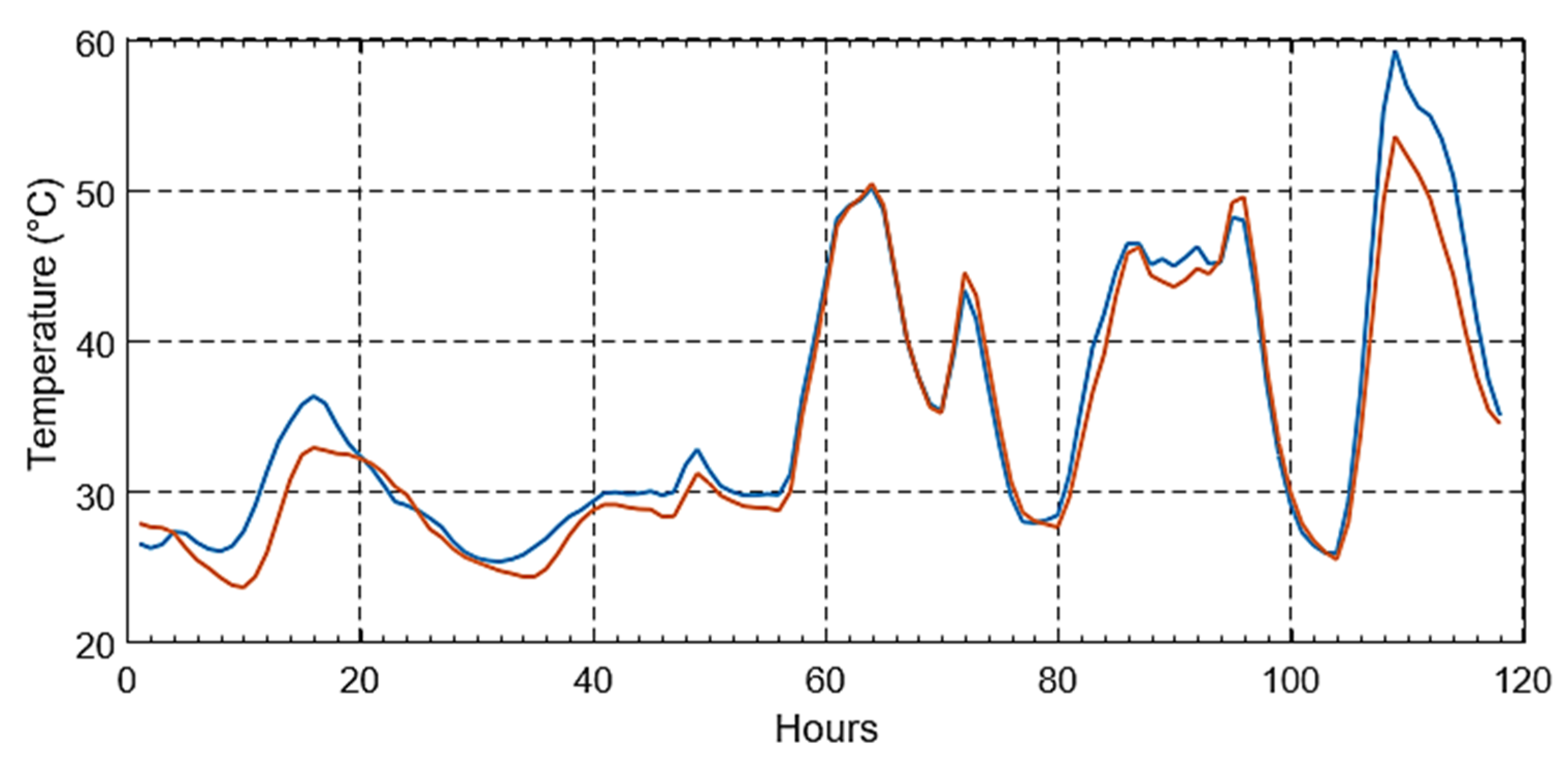
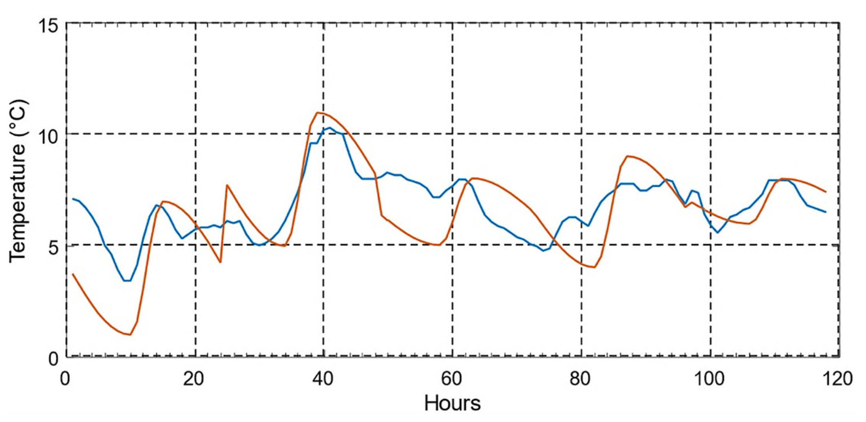
5.8. Application of the Online Diagnostic Thermal Model
5.9. Model for Estimating the Water Content of the Insulation (Paper and Cardboard) and Temperature of the Water Bubbles
5.10. Transformer Aging Model
5.11. Load Factor Model
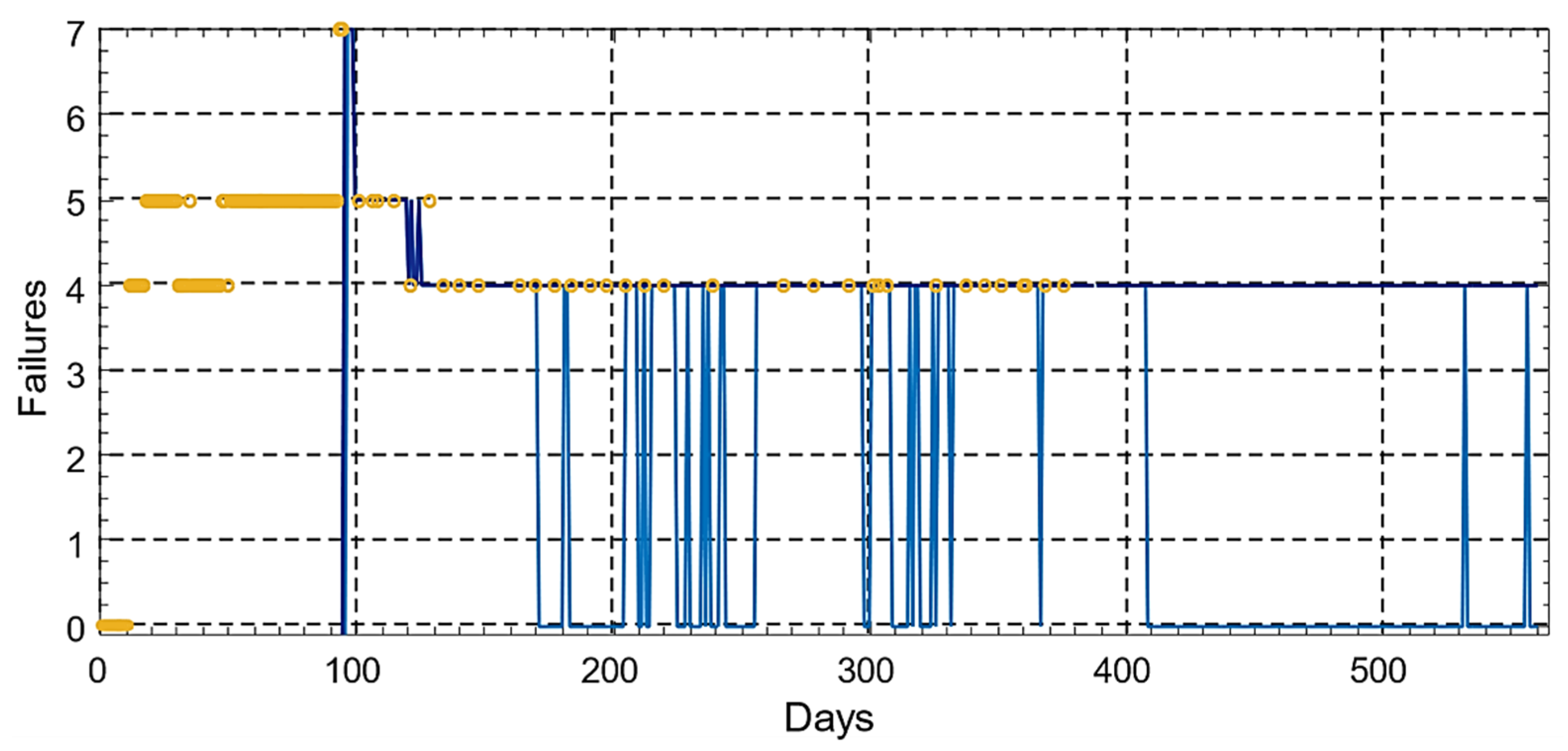
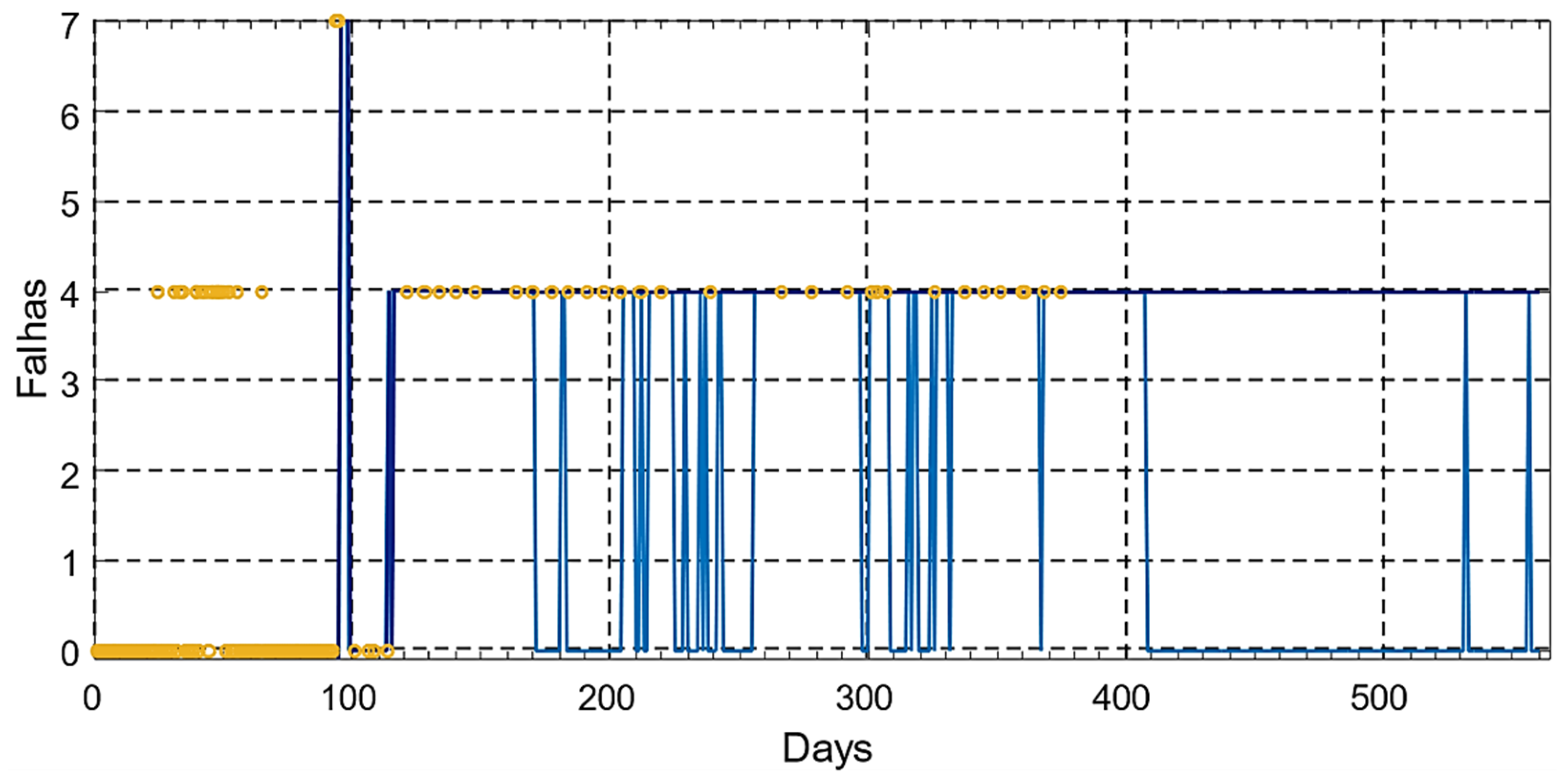
5.12. Model for Analysis of Gases Dissolved in Oil
6. Conclusions
Author Contributions
Funding
Institutional Review Board Statement
Informed Consent Statement
Data Availability Statement
Conflicts of Interest
References
- CIGRE Technical Brochure 248. Economics of Transformer Management; June 2004. Available online: https://e-cigre.org/publication/248-economics-of-transformer-management (accessed on 12 May 2022).
- Office of Electricity Delivery & Energy Reliability. Large Power Transformers and the U.S. Electric Grid; Office of Electricity Delivery & Energy Reliability: Washington, DC, USA, 2012. [Google Scholar]
- USITC. Large Power Transformers from Korea; USITC: Washington, DC, USA, 2011. [Google Scholar]
- Westman, T.; Lorin, P.A.; Ammann, P.A. Keeping aging transformers healthy for longer with ABB TrafoAsset Management–Proactive Services. ABB Rev. 2010, 1, 63–69. [Google Scholar]
- Bossi, A.; Dind, J.E.; Frisson, J.M.; Khoudiakov, U.; Light, F.H.; Narke, D.V.; Tournier, Y.; Verdon, J. An international survey on failures in large power transformers. Cigré Electra 1983, 88, 21–48. [Google Scholar]
- Special Report: Large Power Transformers and the U.S. Electric Grid, the Infrastructure Security and Energy Restoration Office of Electricity Delivery and Energy Reliability, U.S. Department of Energy, June 2012. Available online: https://www.energy.gov/sites/prod/files/Large%20Power%20Transformer%20Study%20-%20June%202012_0.pdf (accessed on 7 March 2022).
- Bohatyrewicz, P.; Mrozik, A. The Analysis of Power Transformer Population Working in Different Operating Conditions with the Use of Health Index. Energies 2021, 14, 5213. [Google Scholar] [CrossRef]
- Aslam, M.; Haq, I.U.; Rehan, M.S.; Ali, F.; Basit, A.; Khan, M.I.; Arbab, M.N. Health Analysis of Transformer Winding Insulation Through Thermal Monitoring and Fast Fourier Transform (FFT) Power Spectrum. IEEE Access 2021, 9, 114207–114217. [Google Scholar] [CrossRef]
- Bagheri, M.; Naderi, M.S.; Blackburn, T.; Phung, T. FRA vs. short circuit impedance measurement in detection of mechanical defects within large power Transformer. In Proceedings of the Conference Record of the IEEE International Symposium on Electrical Insulation (ISEI), San Juan, PR, USA, 10–13 June 2012; pp. 301–305. [Google Scholar]
- Wang, S.; Wang, S.; Cui, Y.; Long, J.; Ren, F.; Ji, S.; Wang, S. An Experimental Study of the Sweep Frequency Impedance Method on the Winding Deformation of an Onsite Power Transformer. Energies 2020, 13, 3511. [Google Scholar] [CrossRef]
- Cong, H.; Pan, H.; Hu, X.; Zhang, M.; Li, Q. Micro-mechanism study on synergistic degradation of the oil-paper insulation with dibenzyl disulfide, hexadecyl mercaptan and benzothiophene. High Volt. 2020, 6, 448–459. [Google Scholar] [CrossRef]
- Sweetser, C. Power Transformer Diagnostics: Novel Techniques and their Application. In Proceedings of the OMICRON, Technical Meeting, 2016. Available online: https://pt.scribd.com/document/400147838/Charles-Sweetser-XFMR-Testing (accessed on 12 May 2022).
- Teymouri; Ashkan; Vahidi, B. Power transformer cellulosic insulation destruction assessment using a calculated index composed of CO, CO 2, 2-Furfural, and Acetylene. Cellulose 2021, 28, 489–502. [Google Scholar] [CrossRef]
- Brandtzæg, G. Health Indexing of Norwegian Power Transformers. Thesis in Engineering of Energy and Environment. Master’s Thesis, Norwegian University of Science and Technology, Trondheim, Norway, 2015. [Google Scholar]
- Ansari, M.A.; Martin, D.; Saha, T.K. Advanced Online Moisture Measurements in Transformer Insulation Using Optical Sensors. IEEE Trans. Dielectr. Electr. Insul. 2020, 27, 1803–1810. [Google Scholar] [CrossRef]
- Adusumilli, P.; Sundar, S.V.N.J. A new criterion for optimal dielectric design of high voltage bushing internal shields in large power transformer. In Proceedings of the 2019 International Conference on High Voltage Engineering and Technology (ICHVET), Hyderabad, India, 7–8 February 2019. [Google Scholar]
- Xie, Q.; He, C.; Yang, Z.; Wen, J. Tests and analyses on failure mechanism of 1100 kV UHV transformer porcelain bushing. High Volt. Eng. 2017, 43, 3154–3162. [Google Scholar]
- Walczak, K.; Gielniak, J. Temperature Distribution in the Insulation System of Condenser-Type HV Bushing—Its Effect on Dielectric Response in the Frequency Domain. Energies 2021, 14, 4016. [Google Scholar] [CrossRef]
- Wang, D.; Zhou, L.; Yang, Z.; Liao, W.; Wang, L.; Guo, L. Simulation for transient moisture distribution and effects on the electric field in stable condition: 110 kV oil-immersed insulation paper bushing. IEEE Access 2019, 7, 162991–163002. [Google Scholar] [CrossRef]
- Li, S.; Yang, L.; Li, S.; Zhu, Y.; Cui, H.; Yan, W.; Ge, Z.; Abu-Siada, A. Effect of AC-voltage harmonics on oil impregnated paper in transformer bushings. IEEE Trans. Dielectr. Electr. Insul. 2020, 27, 26–32. [Google Scholar] [CrossRef]
- Liu, J.; Yang, S.; Zhang, Y.; Zheng, H.; Shi, Z.; Zhang, C. A modified X-model of the oil-impregnated bushing including non-uniform thermal aging of cellulose insulation. Cellulose 2020, 27, 4525–4538. [Google Scholar] [CrossRef]
- Redmil, Presentation on the Slideshare Website. Available online: http://pt.slideshare.net/rezzmk/redmil-powerpoint (accessed on 20 December 2015).
- Ndiaye, I.; Betancourt Ramírez, E.; Avila Montes, J.; Jiang, Y.; Elasser, A. Grid Ready, Flexible Large Power Transformer; No. Final Technical Report: DE-OE0000852; GE Global Research: Niskayuna, NY, USA, 2019. [Google Scholar]
- Dohnal, D. On-Load Tap-Changers for Power Transformers; Maschinenfabrik Reinhausen GmbH Falkensteinstrasse: Regensburg, Gemany, 2013; Volume 8, p. 93059. [Google Scholar]
- Handley, B.; Redfern, M.; White, S. On load tap-changer conditioned based maintenance. IEE Proc.-Gener. Transm. Distrib. 2001, 148, 296–300. [Google Scholar] [CrossRef]
- Al-Ameri, S.M.; Alawady, A.A.; Yousof MF, M.; Kamarudin, M.S.; Illias, H.A. The Effect of Tap Changer Coking and Pitting on Frequency Response Analysis Measurement of Transformer. In Proceedings of the 2021 IEEE International Conference on the Properties and Applications of Dielectric Materials (ICPADM), Johor Bahru, Malaysia, 12–14 July 2021. [Google Scholar]
- Seo, J. Intelligent condition monitoring and diagnosis of a power transformer: On-load tap changer (OLTC) and main winding. Ph.D. Thesis, The University of Queensland, St Lucia, Australia, 2019. [Google Scholar]
- Saha, T.K.; Purkait, P. (Eds.) Transformer Ageing: Monitoring and Estimation Techniques; John Wiley & Sons: Hoboken, NJ, USA, 2017. [Google Scholar]
- Brodeur, S.; Lê Van, N.; Champliaud, H. A nonlinear finite-element analysis tool to prevent rupture of power transformer tank. Sustainability 2021, 13, 1048. [Google Scholar] [CrossRef]
- Jahromi, A.; Piercy, R.; Cress, S.; Service, J.; Fan, W. An approach to power transformer asset management using health index. IEEE Electr. Insul. Mag. 2009, 25, 20–34. [Google Scholar] [CrossRef]
- Wang, R.; Zhang, Y.; Jiao, B. Theory research on high performance control technology of large power transformer strong oil-cooled system. In Proceedings of the 2020 IEEE 4th Information Technology, Networking, Electronic and Automation Control Conference (ITNEC), Chongqing, China, 12–14 June 2020; Volume 1. [Google Scholar]
- Kim, Y.J.; Jeong, M.; Park, Y.G.; Ha, M.Y. A numerical study of the effect of a hybrid cooling system on the cooling performance of a large power transformer. Appl. Therm. Eng. 2018, 136, 275–286. [Google Scholar] [CrossRef]
- Gao, X.; Schlosser, C.A.; Morgan, E.R. Potential impacts of climate warming and increased summer heat stress on the electric grid: A case study for a large power transformer (LPT) in the Northeast United States. Clim. Chang. 2018, 147, 107–118. [Google Scholar] [CrossRef] [Green Version]
- Weiping, M.; Fangxiao, C.; Ying, S.; Chungui, X.; Ming, A. Fault diagnosis on power transformers using non-electric method. In Proceedings of the 2006 IEEE International Symposium on Industrial Electronics, Montreal, QC, Canada, 9–13 July 2006; Volume 3. [Google Scholar]
- Franzén, A.; Karlsson, S. Failure Modes and Effects Analysis of Transformers; Royal Institute of Technology, KTH School of Electrical Engineering: Stockholm, Sweden, 2007. [Google Scholar]
- Eyüboğlu, O.H.; Dindar, B.; Gül, Ö. Risk Assessment by Using Failure Modes and Effects Analysis (FMEA) Based on Power Transformer Aging for Maintenance and Replacement Decision. In Proceedings of the 2020 2nd Global Power, Energy and Communication Conference (GPECOM), Izmir, Turkey, 20–23 October 2020. [Google Scholar]
- Ciulavu, C.; Helerea, E. Power transformer incipient faults monitoring. Ann. Univ. Craiova–Electr. Eng. Ser. 2008, 32, 72–77. [Google Scholar]
- Bustamante, S.; Manana, M.; Arroyo, A.; Laso, A.; Martinez, R. Determination of Transformer Oil Contamination from the OLTC Gases in the Power Transformers of a Distribution System Operator. Appl. Sci. 2020, 10, 8897. [Google Scholar] [CrossRef]
- Hussain, M.R.; Refaat, S.S.; Abu-Rub, H. Overview and Partial Discharge Analysis of Power Transformers: A Literature Review. IEEE Access 2021, 9, 64587–64605. [Google Scholar] [CrossRef]
- IEC 60599:2015; Mineral Oi-Impregnated Electrical Equipment in Services-Guide to the Interpretation of Dissolved and Free Gases Analysis. Interna-tional Standard TC 10. IEC: Geneva, Switzerland, 2015.
- Qi, B.; Zhang, P.; Rong, Z.; Li, C. Differentiated warning rule of power transformer health status based on big data mining. Int. J. Electr. Power Energy Syst. 2020, 121, 106150. [Google Scholar] [CrossRef]
- IEEE Standard C57.104-2008; IEEE Guide for the Interpretation of Gases Generated in Oil-Immersed Transformers. IEEE: Piscataway, NJ, USA, 2008.
- Cheng, L.; Yu, T. Dissolved Gas Analysis Principle-Based Intelligent Approaches to Fault Diagnosis and Decision Making for Large Oil-Immersed Power Transformers: A Survey. Energies 2018, 11, 913. [Google Scholar] [CrossRef] [Green Version]
- Cheng, L.; Yu, T.; Wang, G.; Yang, B.; Zhou, L. Hot Spot Temperature and Grey Target Theory-Based Dynamic Modelling for Reliability Assessment of Transformer Oil-Paper Insulation Systems: A Practical Case Study. Energies 2018, 11, 249. [Google Scholar] [CrossRef] [Green Version]
- de Faria, H., Jr.; SpirCosta, J.G.; Olivas, J.L.M. A review of monitoring methods for predictive maintenance of electric power transformers based on dissolved gas analysis. Renew. Sustain. Energy Rev. 2015, 46, 201–209. [Google Scholar] [CrossRef]
- Hydroelectric Research and Technical Services Group. Transformer Diagnostics; United States Department of the Interior Bureau of Reclamation: Washington, DC, USA, 2003. [Google Scholar]
- DGA Diagnostic Methods, Serveron White Paper, PN 880-0129-00 Rev. B, Serveron Corporation: Hillsboro, OH, USA, 2007.
- Atanasova-Höhlein, I. DGA–Method in the Past and for the Future; 2012. Available online: https://assets.new.siemens.com/siemens/assets/api/uuid:d9fa9803-8a7b-46c0-a9e9-ba0c7af71c29/dga-method-in-the-past-and-for-the-future.pdf (accessed on 23 June 2022).
- Dukarm, J.; Draper, Z.; Piotrowski, T. Diagnostic Simplexes for Dissolved-Gas Analysis. Energies 2020, 13, 6459. [Google Scholar] [CrossRef]
- Tahir, M. Intelligent Condition Assessment of Power Transformer Based on Data Mining Techniques Master Thesis. Master’s Thesis, University of Waterloo, Waterloo, ON, Canada, 2012. [Google Scholar]
- Pickster, K. Determination of Probability of Failure of Power Transformers using Statistical Analysis. Master’s Thesis, University of the Witwatersrand, Johannesburg, South Africa, 2015. [Google Scholar]
- IEEE Standard C57.106-2006; IEEE Guide for Acceptance and Maintenance of Insulating Oil in Equipment. IEEE: Piscataway, NJ, USA, 2006.
- Sumereder, C.; Muhr, M. Moisture Determination and Degradation of Solid Insulation System of Power Transformers. In Proceedings of the 2010 IEEE International Symposium on Electrical Insulation, San Diego, CA, USA, 6–9 June 2010; pp. 1–4. [Google Scholar] [CrossRef]
- Prevost, T. New Techniques for the Monitoring of Transformer Condition. In Proceedings of the IEEE T&D Conference, Chicago, IL, USA, 17 April 2014. [Google Scholar]
- Mohamed, E.A.; Abdelaziz, A.Y.; Mostafa, A.S. A neural network-based scheme for fault diagnosis of power transformers. Electr Power Syst. Res. 2005, 75, 29–39. [Google Scholar]
- Barle, N.; Jha, M.K.; Qureshi, M.F. Artificial Intelligence Based Fault Diagnosis of Power Transformer-A Probabilistic Neural Network and Interval Type-2 Support Vector Machine Approach. International Journal of Innovative Research in Science. Eng. Technol. 2015, 4, 71–89. [Google Scholar]
- Ahmed, M.R.; Geliel, M.A.; Khalil, A. Power Transformer Fault Diagnosis using Fuzzy Logic Technique Based on Dissolved Gas Analysis. In Proceedings of the 21st Mediterranean Conf. Control Automat. Platanias, Greece, 25–28 June 2013; pp. 584–589. [Google Scholar]
- Oliveira, L.M.R. Desenvolvimento de Métodos de Deteção de Avarias e Algoritmos de Proteção para Aplicação em Sistemas de Monitorização Contínua de Transformadores Trifásicos, Tese de Doutoramento; Faculdade de Ciências e Tecnologia da Universidade de Coimbra: Coimbra, Portuga, 2013. [Google Scholar]
- Myers, C. Transformer Conditioning Monitoring by Oil Analysis Large or Small; Contaminant or Catastrophe, in proc. In Proceedings of the First IEE/IMechE International Conference on Power Station Maintenance-Profitability Through Reliability, Edinburgh, UK, 30 March–1 April 1998. [Google Scholar]
- “Engineering Photos, Videos and Articles (Engineering Search Engine)”, Chapter 1 Power Transformers. Posted on December 2012. Available online: http://emadrlc.blogspot.pt/2012/12/chapter-1-power-transformers.html (accessed on 10 August 2016).
- Jan, S.T.; Afzal, R.; Khan, A.Z. Transformer Failures, Causes & Impact. In Proceedings of the International Conference Data Mining, Civil and Mechanical Engineering, Bali, Indonesia, 1–2 February 2015. [Google Scholar]
- Singh, R.; Zadgaonkar, A.S.; Singh, A. Premature Failure of Distribution Transformers-A Case Study. Int. J. Sci. Eng. Res. 2014, 5, 1457–1466. [Google Scholar]
- University of Coimbra, Physics Departament. Available online: http://www.fis.uc.pt/data/20072008/apontamentos/apnt_330_15.pdf (accessed on 20 December 2015).
- Technical Brochure No. 227 Guidelines for Life Management Techniques for Power Transformers. CIGRE WG 12.18; Life Management of Transformers: Paris, France, 2022; p. 125.
- Soares, M.A. Elementos Para a Gestão do Ciclo de Vida de Transformadores Elétricos de Potência, Tese de Mestrado; FEUP: Porto, Portugal, 2011. [Google Scholar]
- ABB, Site da ABB. 2016. Available online: http://new.abb.com/products/transformers/transformer-components/ac-bushings-iec/oil-to-air-application/ac-bushings-type-gob (accessed on 20 July 2016).
- Feilat, E.A.; Metwally, I.A.; Al-Matri, S.; Al-Abri, A.S. Analysis of the Root Causes of Transformer Bushing Failures. Int. J. Comput. Electr. Autom. Control Inf. Eng. 2013, 7, 791–796. [Google Scholar]
- MR, Site da MR. Available online: http://www.reinhausen.com/desktopdefault.aspx/tabid-1551/179_read-335/ (accessed on 15 June 2016).
- Franzén, A.; Karlsson, S. Failure Modes and Effects Analysis of Transformers Technical Report TRITA-EE 2007:040; KTH School of Electrical Engineering: Zurich, Switzerland, 2007. [Google Scholar]
- Weather Underground Site. Available online: https://www.wunderground.com (accessed on 2 March 2022).


| Component | Failure Mode | Event | Cause |
|---|---|---|---|
| Core | Loss of efficiency | Blade displacement | —Eddy currents |
| Windings | Short-circuit | Mechanical damage | —Manufacturing deficiencies —Corrosion —Bad maintenance —Vibrations —Mechanical displacements |
| Insulation Failure | —Overvoltage —Overheating | ||
| Solid insulation | Cannot provide insulation | Mechanical damage | —Cellulose aging |
| Insulation Failure | —Cellulose Aging —Overheating | ||
| Insulation fluids | Short-circuit | Conductive particles in the oil | —Aging —Overheating |
| Overheating | Oil does not cool | —Pumps/Fans failure —Particles in oil (aging and overheating) | |
| Bushings | Overheating | Partial discharges and loss of dielectric properties | —Insulator contamination —Water inlet —Aging |
| On-load voltage regulator | Inability to change the number of turns ratio | Mechanical damage | —Breakage of springs —Lack of maintenance —Old or burnt condensers —Carbonization —Switching system wear |
| Oil tank | Oil leakage | Damage to tank walls | —High gas pressure —Environmental wear |
| Cooling system | Overheating | Cooling incapacity | —Pipe cracks —Particles in oil (aging and overheating) —Pump/fan failures |
| Cause | Failure | |||
|---|---|---|---|---|
| Paper Overheating | Oil Overheating | High Energy Electrical Discharge | Low Energy Electrical Discharge | |
| Short circuit between turns of the windings | X | X | ||
| Winding open circuit | X | X | ||
| Internal LTC Operation | X | |||
| Deformation or displacement of windings | X | X | ||
| Loss of connection of the crossing terminals | X | X | X | |
| Water or too much moisture in the oil | X | X | ||
| Metallic particles in the oil | X | X | ||
| Displacement of spacers | X | |||
| Overload | X | |||
| Insulation between blades damaged | X | |||
| Rust or other core damage | X | |||
| Obstacles to the passage of oil | X | |||
| Cooling system malfunction | X | |||
| Failure | H2 | CH4 | C2H6 | C2H4 | C2H2 | CO | CO2 |
|---|---|---|---|---|---|---|---|
| Thermal paper |  |  | |||||
| Thermal oil (150–300 °C) |  |  |  |  | |||
| Thermal oil (300–700 °C) |  |  |  |  |  | ||
| Thermal oil (>700 °C) |  |  |  |  |  | ||
| Low energy discharge |  |  |  |  | |||
| High energy discharge (Arc-electric) |  |  |  |  | |||
| Partial discharge |  |  |  |  |
| Abbreviation | Failure | R2 (C2H2/C2H4) | R1 (CH4/H2) ou C2H2/C2H6 | R5 (C2H4/C2H6) |
|---|---|---|---|---|
| PD | Partial Discharges | Negligible value | R < 0.1 | R < 0.2 |
| D1 | Low Energy Discharges | 1.0 < R | 0.1 < R < 0.5 | 1.0 < R |
| D2 | High Energy Discharges | 0.6 < R < 2.5 | 0.1 < R < 1.0 | 2.0 < R |
| T1 | Thermal Failure T < 300 °C | Negligible value | Negligible value | 1.0 < R |
| T2 | Thermal Failure 300 °C < T < 700 °C | R < 0.1 | 1.0 < R | 1.0 < R < 4.0 |
| T3 | Thermal Failure T < 700 °C | R < 0.2 | 1.0 < R | 4.0 < R |
| Key Gases | Failures | Typical Emission Proportion |
|---|---|---|
| H2 andC2H2 | High energy electrical discharge | Large amounts of H2 and C2H2. Small quantities of CH4 and C2H4. The formation of CO2 e CO indicates paper combustion. |
| C2H4 | Oil overheating | Mainly C2H4. Reduced quantities of C2H6, CH4, and H2. Residues of C2H2, with large temperature failures. |
| CO | Paper overheating | Mainly CO and CO2. |
| H2 | Electrolysis | Mainly H2. |
| H2 | High energy electrical discharge, partial discharge | Mainly H2. Small amounts of CH4. Trace elements of C2H4 and C2H6. |
| Gases | Limit L1 (ppm) |
|---|---|
| H2 | 100 |
| CH4 | 120 |
| CO | 350 |
| C2H2 | 35 |
| C2H4 | 50 |
| C2H6 | 65 |
| TDCG Level (ppm) | TDCG Generation Rates (ppm/Day) | Sampling Intervals and Operating Actions for Gas Generation Rates | |
|---|---|---|---|
| Sampling Interval | Operating Procedures | ||
| <720 | <10 | Twice a year | Continue normal operation. |
| 10–30 | Quarterly | ||
| >30 | Monthly | Caution is necessary. Analyze individual gases to find the cause. Determine load dependence. | |
| 721–1920 | <10 | Quarterly | Caution is extremely necessary. Analyze individual gases to find the cause. Determine load dependence. |
| 10–30 | Monthly | ||
| >30 | |||
| 1921–4630 | <10 | Monthly | Exercise extreme caution. Analyze individual gases to find the cause. Plan outage. |
| 10–30 | Weekly | ||
| >30 | |||
| >4630 | <10 | Weekly | Exercise extreme caution. Analyze individual gases to find the cause. Plan outage. |
| 10–30 | Daily | ||
| >30 | Consider removal from service. | ||
| Ratio R1 (CH4/H2) | Ratio R2 (C2H2/C2H4) | Ratio R5 (C2H4/C2H6) | Failure |
|---|---|---|---|
| 0.1 < R < 1.0 | R < 0.1 | R < 1.0 | Normal operation. |
| R < 0.1 | R < 0.1 | R < 1.0 | Low energy electrical discharge |
| 0.1 < R < 1.0 | 1.0 < R < 3.0 | 3.0 > R | High-energy electrical discharge |
| 0.1 < R < 1.0 | R < 0.1 | 1.0 < R < 3.0 | Low temperature thermal failure |
| 1.0 > R | R < 0.1 | 1.0 < R < 3.0 | Thermal failure <700 °C |
| 1.0 > R | R < 0.1 | 3.0 > R | Thermal failure >700 °C |
| Test | Standard/ ASTM Method | IEC |
|---|---|---|
| Color | ASTM D1500 | ISSO 2049 |
| Interfacial Tension | ASTM D971 | ISSO 6295 |
| Visual inspection | ASTM D1524 | - |
| Breakdown voltage | ASTM D1816 | IEC60156 |
| Dissipation factor | ASTM D924 | IEC247 |
| Neutralizing number | ASTM D664 | IEC62021 |
| Water content | ASTM D1533 | IEC60814 |
| Test | Value According to Voltage Classes | ||
|---|---|---|---|
| ≤69 kV | 69–230 kV | ≥230 kV | |
| Dielectric breakdown voltage [kV] for 1mm electrode distance (minimum value) | 23 | 28 | 30 |
| Interfacial tension [mN/m] (minimum value) | 25 | 30 | 32 |
| Neutralizing number [mg KOH/g] (maximum value) | 0.2 | 0.15 | 0.1 |
| Water content [ppm] (maximum value) | 35 | 25 | 20 |
| Test Measure | ONAN (“Oil Natural Air Natural”) | ONAF (“Oil Natural Air Forced”) | OF (a) (“Oil Forced”) | OD (b) (“Oil-Directed”) |
|---|---|---|---|---|
| x | 0.8 | 0.8 | 1.0 | 1.0 |
| y | 1.3 | 1.3 | 1.3 | 2.0 |
| R | 6.0 | 6.0 | 6.0 | 6.0 |
| (min) | 210 | 150 | 90 | 90 |
| 10 | 7 | 7 | 7 | |
| (K) | 52 | 52 | 56 | 49 |
| (K) | 26 | 26 | 22 | 29 |
| k11 | 0.5 | 0.5 | 1.0 | 1.0 |
| k21 | 2.0 | 2.0 | 1.3 | 1.0 |
| k22 | 2.0 | 2.0 | 1.0 | 1.0 |
| Insulation | 40 °C | 80 °C | ||
|---|---|---|---|---|
| Oil (25,000 L) | 10 ppm | 0.25 kg | 80 ppm | 2.0 kg |
| Paper (2500 kg) | 3 % | 75 kg | 2.93% | 73.25 kg |
| Total | 75.25 kg | 75.25 kg | ||
| Oil | Paper | A | B |
|---|---|---|---|
| Shell Diala D (new) | New | 195.5 | −0.11186 |
| Shell Diala D (new) | Improved. thermally new | 237.7 | −0.13718 |
| Shell Diala K 6 SX (used) | Improved. thermally used | 178 | −0.07338 |
| Paper Type | Oxygen Concentration in Oil | Water Content on Paper | A |
|---|---|---|---|
| Kraft paper | Low | 0.5% | 1.42 (108) |
| 1.6% | 6.80 (108) | ||
| 2.7% | 1.65 (109) | ||
| Average | 0.5% | 4.66 (108) | |
| 1.6% | 1.66 (109) | ||
| 2.7% | 3.33 (109) | ||
| High | 0.5% | 9.33 (108) | |
| 1.6% | 3.05 (109) | ||
| 2.7% | 4.70 (109) | ||
| Thermally improved kraft paper | Low | 0.5% | 6.92 (107) |
| 1.6% | 2.61 (108) | ||
| 2.7% | 1.03 (109) | ||
| Average | 0.5% | 2.70 (108) | |
| 1.6% | 7.32 (108) | ||
| 2.7% | 2.03 (109) | ||
| High | 0.5% | 4.29 (108) | |
| 1.6% | 2.03 (109) | ||
| 2.7% | 4.27 (109) |
| Standard | Gas Concentration [ppm] | |||||||
|---|---|---|---|---|---|---|---|---|
| H2 | CO | CO2 | CH4 | C2H6 | C2H4 | C2H2 | TCG | |
| IEC Std 60599-97 | 60–150 | 540–900 | 5100–13,000 | 40–110 | 50–90 | 60–280 | 3–50 | - |
| IEEE Std C57.104–91 | 100 | 350 | 2500 | 120 | 65 | 50 | 1 | 720 |
| Laborelec | 200 | - | - | Σ CnHy < 300 | - | |||
| CIGRE 15.01 | 100 | Σ CO + CO2 < 10,000 | - | - | - | 20 | - | |
| Σ CnHy < 500 | - | |||||||
| Type of Bushings | Power Factor (cos θ) Corrected to 20 °C | Capacity | |
|---|---|---|---|
| Limit [%] | Acceptable Change | Acceptable Change [%] | |
| OIP | 0.5 | +0.02/−0.04 | ±1.0 |
| RIP | 0.85 | ±0.04 | ±1.0 |
| RBP | 2.0 | ±0.08 | ±1.0 |
| Abnormal Operating Conditions | Measurements/Testes | |||||
|---|---|---|---|---|---|---|
| Temperature | Analysis of Gases Dissolved in Oil | Motor Electric Current | Vibrations | |||
| Resistance | Reactance | Vacuum | ||||
| Contact wear | X | X | X | |||
| Overheating | X | X | X | X | X | |
| Transition timing | X | X | X | |||
| Alignment contacts | X | X | X | X | ||
| Electric arc | X | X | X | X | ||
| Sequence/Timing | X | X | X | |||
| Motor | X | |||||
| Brake | X | |||||
| Lubrication | X | |||||
| Control/Relays | X | |||||
| Connections/Gears | X | X | X | X | ||
| H2 | ±25 ppm |
| C2H2 | ±5 ppm |
| C2H4 | ±10 ppm |
| CO | ±25 ppm |
| H2O | ±3 ppm |
| Quantity | Norma |
|---|---|
| Gases | IEC 60567 |
| Water | IEC 60814 |
| Furans | IEC 61198 |
| Color and appearance | ISO 2049 |
| Density (20 °C) | ASTM D4052 |
| Neutralizing number | IEC 62021-1 |
| Breakdown voltage | IEC 60156 |
| Dissipation factor | IEC 60247 |
| Phenolic inhibitor | IEC 60666 |
| Sludge and sediment | IEC 60422 |
| Gases | Error Root Mean Square (ERMS) | Absolute Mean Error (AEM) | Relative Mean Error (RME) |
|---|---|---|---|
| C2H2 | 3.07 ppm | 2.35 ppm | 8.01% |
| C2H4 | 45.93 ppm | 34.77 ppm | 9.6% |
| H2 | 43.93 ppm | 40.22 ppm | 25.0% |
| CO | 5.48 ppm | 4.45 ppm | 14.91% |
| January | August | |
|---|---|---|
| Error Root Mean Square (ERMS) | 1.5 °C | 2.3 °C |
| Absolute Mean Error (AEM) | 1.25 °C | 1.63 °C |
| Relative Mean Error (RME) | 20.18% | 8.53% |
| January | August | |
|---|---|---|
| Error Root Mean Square (ERMS) | 1.51 °C | 2.17 °C |
| Absolute Mean Error (AEM) | 1.16 °C | 1.54 °C |
| Relative Mean Error (RME) | 4.79% | 3.74% |
| H2 | O2 | N2 | CO | CO2 | CH4 | C2H4 | C2H6 | C2H2 | |
|---|---|---|---|---|---|---|---|---|---|
| H2 | 1.00 | −0.057 | 0.033 | 0.347 | 0.433 | 0.635 | 0.576 | 0.6353 | 0.717 |
| O2 | −0.057 | 1.00 | 0.913 | 0.1922 | 0.308 | −0.143 | −0.150 | −0.126 | 0.0486 |
| N2 | 0.033 | 0.914 | 1.00 | 0.288 | 0.399 | −0.15 | −0.167 | −0.129 | 0.135 |
| CO | 0.347 | 0.192 | 0.2885 | 1.00 | 0.794 | −0.293 | −0.348 | −0.275 | 0.387 |
| CO2 | 0.433 | 0.308 | 0.399 | 0.794 | 1.00 | 0.021 | 0.002 | 0.056 | 0.553 |
| CH4 | 0.635 | −0.143 | −0.151 | −0.29 | 0.021 | 1.00 | 0.993 | 0.994 | 0.332 |
| C2H4 | 0.576 | −0.15 | −0.168 | −0.348 | 0.002 | 0.993 | 1.00 | 0.989 | 0.319 |
| C2H6 | 0.635 | −0.126 | −0.129 | −0.275 | 0.057 | 0.994 | 0.989 | 1.00 | 0.327 |
| C2H2 | 0.717 | 0.048 | 0.135 | 0.387 | 0.553 | 0.332 | 0.31 | 0.327 | 1.00 |
| Gases | Error Root Mean Square (ERMS) | Absolute Mean Error (AEM) | Relative Mean Error (RME) |
|---|---|---|---|
| CH4 | 40.24 ppm | 30.85 ppm | 10.13% |
| C2H6 | 8.3 ppm | 6.82 ppm | 9.75% |
| CO2 | 23.13 ppm | 17.95 ppm | 6.93% |
| Code | Failure Type |
|---|---|
| 0 | No failure |
| 1 | partial discharges |
| 2 | Thermal [150–300 °C] |
| 3 | Thermal [300–700 °C] |
| 4 | Thermal [>700 °C] |
| 5 | Electrical evasion and thermal failure |
| 6 | low energy discharge |
| 7 | High energy discharge (Arc-electric) |
Publisher’s Note: MDPI stays neutral with regard to jurisdictional claims in published maps and institutional affiliations. |
© 2022 by the authors. Licensee MDPI, Basel, Switzerland. This article is an open access article distributed under the terms and conditions of the Creative Commons Attribution (CC BY) license (https://creativecommons.org/licenses/by/4.0/).
Share and Cite
Costa, J.V.; Silva, D.F.F.d.; Branco, P.J.C. Large-Power Transformers: Time Now for Addressing Their Monitoring and Failure Investigation Techniques. Energies 2022, 15, 4697. https://doi.org/10.3390/en15134697
Costa JV, Silva DFFd, Branco PJC. Large-Power Transformers: Time Now for Addressing Their Monitoring and Failure Investigation Techniques. Energies. 2022; 15(13):4697. https://doi.org/10.3390/en15134697
Chicago/Turabian StyleCosta, Jonathan Velasco, Diogo F. F. da Silva, and Paulo J. Costa Branco. 2022. "Large-Power Transformers: Time Now for Addressing Their Monitoring and Failure Investigation Techniques" Energies 15, no. 13: 4697. https://doi.org/10.3390/en15134697
APA StyleCosta, J. V., Silva, D. F. F. d., & Branco, P. J. C. (2022). Large-Power Transformers: Time Now for Addressing Their Monitoring and Failure Investigation Techniques. Energies, 15(13), 4697. https://doi.org/10.3390/en15134697