CVR Study and Active Power Loss Estimation Based on Analytical and ANN Method

Abstract

Conservation through voltage reduction (CVR) aims to reduce the peak load and energy savings in electric power systems and is being deployed at various utilities. The effectiveness of the CVR program depends on the load characteristics, i.e., the sensitivity of the load to voltage variation, and voltage regulation device settings. In the current literature, there is a lack of discussion on the CVR factor calculation using different measurements, and there is a lack of method for active power loss estimation using substation measurements. This paper provides insights into CVR factor calculation based on the measurements captured at the substation and those at the load location. This paper also proposes a new method based on curve fitting and artificial neural network to estimate the active power loss using input active power, input reactive power and input voltage at the substation. The CVR comparison study conducted in this paper helps in understanding the factors affecting CVR factor and may provide guidance in CVR implementation and impact assessment. The proposed loss estimation method sheds light on the impacts of CVR in terms of load and loss reduction. The results based on simulation studies using the IEEE 13-bus and 34-bus systems are reported in this paper, noting that the proposed methods are applicable to larger systems, as long as the required measurements at the substation are available. Future research includes testing and refining the methods using large IEEE and utility distribution systems and considering the stochastic nature of the CVR factor with changing load and voltage regulator control schemes.

1. Introduction

The world is currently experiencing a massive surge in energy demand, due to various demographic, environmental and economic reasons. When facing high demand, the electric distribution companies have two options to manage the demand. The first option is to arrange supply for the demand, which may not be available each time. The second option is to curtail the peak load, which may be a more viable method. This reduction may be achieved by decreasing the voltage level on the distribution feeder line. The decrease in the bus voltage leads to a decline in the voltage-dependent load demand, which may also reduce the total energy consumption during a specified time duration. This strategy is called conservation through voltage reduction (CVR) [1]. The objective of CVR is to reduce the peak load or reduce the energy consumption for energy savings, while regulating the voltage within the limit set by the American National Standards Institute (ANSI). ANSI C84.1 standard sets the range for voltages at the secondary terminals of transformer at 120 volts, which can vary by 5% of the aforesaid limit, resulting in a voltage level between 114 and 126 volts [2]. Over the years, numerous CVR-related operations have been conducted in the country, with the earliest being performed by the American Electric Power system (AEP) in 1973 [3]. Afterwards, various utilities, such as Northeast Utilities (NU) [4], Southern California Edison (SCE) [5], and Dominion Virginia Power [6] have performed CVR tests. These tests resulted in a reduction in the load by 0.3% to 1% per 1% voltage reduction. Ref. [7] conducted a study that estimated a 3.04% reduction in annual energy consumption in the case of deployment of CVR on all distribution feeders of the United States. In addition to the USA, other countries, such as Australia [8] and Ireland [9], have also conducted CVR, resulting in 1% and 1.7% energy savings, respectively. CVR is regarded as an efficient method to manage the load demand in distribution power systems [10].

CVR is one of the most viable methods towards ensuring an economic and environmentally sustainable power network, as it provides numerous benefits to the electric utilities and end-use consumers. CVR can reduce carbon emissions and can extend the life of a transformer by reducing its iron losses by decreasing the voltage [11]. Moreover, increase in energy savings will also lead to less maintenance cost, due to the improvement in the life of substation devices and will also increase the lifespan of consumer appliances, such as incandescent lamps and electric water heaters [12]. The aforesaid benefits of CVR can also ensure improvement in the utilization of various assets linked to the power network, reduce energy demand, and increase the energy efficiency [13].

CVR can be implemented using the following two techniques. The first technique is to reduce the voltage by adding capacitors, line-drop-compensators, and load-tap-changers. The second technique involves decreasing the voltage using a supervisory control and data acquisition (SCADA) system and the advance metering infrastructure (AMI) [6,14]. While applying either of the techniques, it is desired to keep the voltage profile as flat as possible. The aforesaid can be achieved by adding capacitors at different sites to increase the power factor and reduce the power loss. The assessment of CVR program performance is crucial, which can be performed using four assessment methods that are simulation-based, comparison-based, synthesis based, and regression-based methods [15,16]. Various studies have been carried out on the assessment of CVR performance. Dominion Virginia Power developed its own method for CVR calculation by aggregating available AMI data with the existing data management system (DMS) controls over a time duration into a single summary record per meter, with analytical support from the geographic information system (GIS) and planning data [6]. Ref. [17] used the adaptive voltage control technique to control the substation voltage by using automatic control and communications. Both constant or time varying impedance, current and power model, i.e., ZIP model, have been used in CVR assessment studies, as well as in demand and loss reduction optimization [18]. Ref. [19] used a regression and simulation method to calculate the CVR factor for a time-varying ZIP load model. A two-stage recursive least squares algorithm under the regression method was used to calculate the CVR factor and a simulation method was used to determine the accuracy of the CVR calculation method. Ref. [20] used the Kalman filtering method to calculate time-varying ZIP parameters. Ref. [21] devised a coordinated voltage control scheme for voltage control for CVR by varying the voltage (near the operating lower voltage limit) at the on-load tap changer (OLTC) at the substation, in coordination with step voltage regulator (SVR) or shunt capacitor banks at feeders. Ref. [22] presented a multi-objective Volt-Var optimization problem. Different target functions were used to express the system state defined by voltage, active power, reactive power, direct and indirect Volt-Var control methods. Ref. [23] performed a case study on the usage of the CVR/VVO method by various electric utilities across USA with specific focus on the utilities, discussing their methodology for CVR factor calculation. They presented a measurement and verification benchmark of CVR/VVO used by several electric utilities in the U.S. Ref. [24] presented an ANN-based model to accurately calculate the measurements for active power, reactive power, and voltage to obtain optimal output values including power loss. Ref. [25] proposed an algorithm based on the Markov chain and Monte Carlo (MCMC) method to accurately identify the parameters including head and end voltages and active and reactive power on the low voltage side of a power distribution network. Ref. [26] presented a selective particle swarm optimization (SPSO) algorithm to solve an optimization model for optimal placement and sizing of distributed generators to reduce the distribution power losses, keeping technical constraints intact.

However, these studies do not provide a detailed CVR analysis considering both the utility and the consumer perspective, while studying the relationship between active power loss, and input voltage, input active and reactive power affecting the CVR factor. Moreover, they do not depict the relationship between active power loss, active power, reactive power, and voltage. This is the research gap that needs to be addressed in this paper. This paper focuses on the calculation of the CVR factor for the IEEE 13-bus and 34-bus systems, using a simulation-based method from the substation and the load perspective. It also attempts to identify the relationship between active power loss and the input quantities affecting the CVR factor calculation and studies the effect of voltage regulator on the CVR factor.

The paper is structured as follows: Section 2 describes the substation and the load perspective used to calculate the CVR factor. Section 3 focuses on the function methodology used to calculate the active power loss $\left(P_{loss}\right)$. It also explains the least squares method used to calculate the constants of the function. Section 4 discusses the artificial neural network (ANN) method used to calculate the $\left(P_{loss}\right)$. Section 5 explains the findings achieved for the work carried out in Section 2, Section 3 and Section 4. Section 6 concludes the methodologies and the results obtained from them. It also explains the future scope of this research.

2. CVR Factor Estimation Based on Simulation Studies

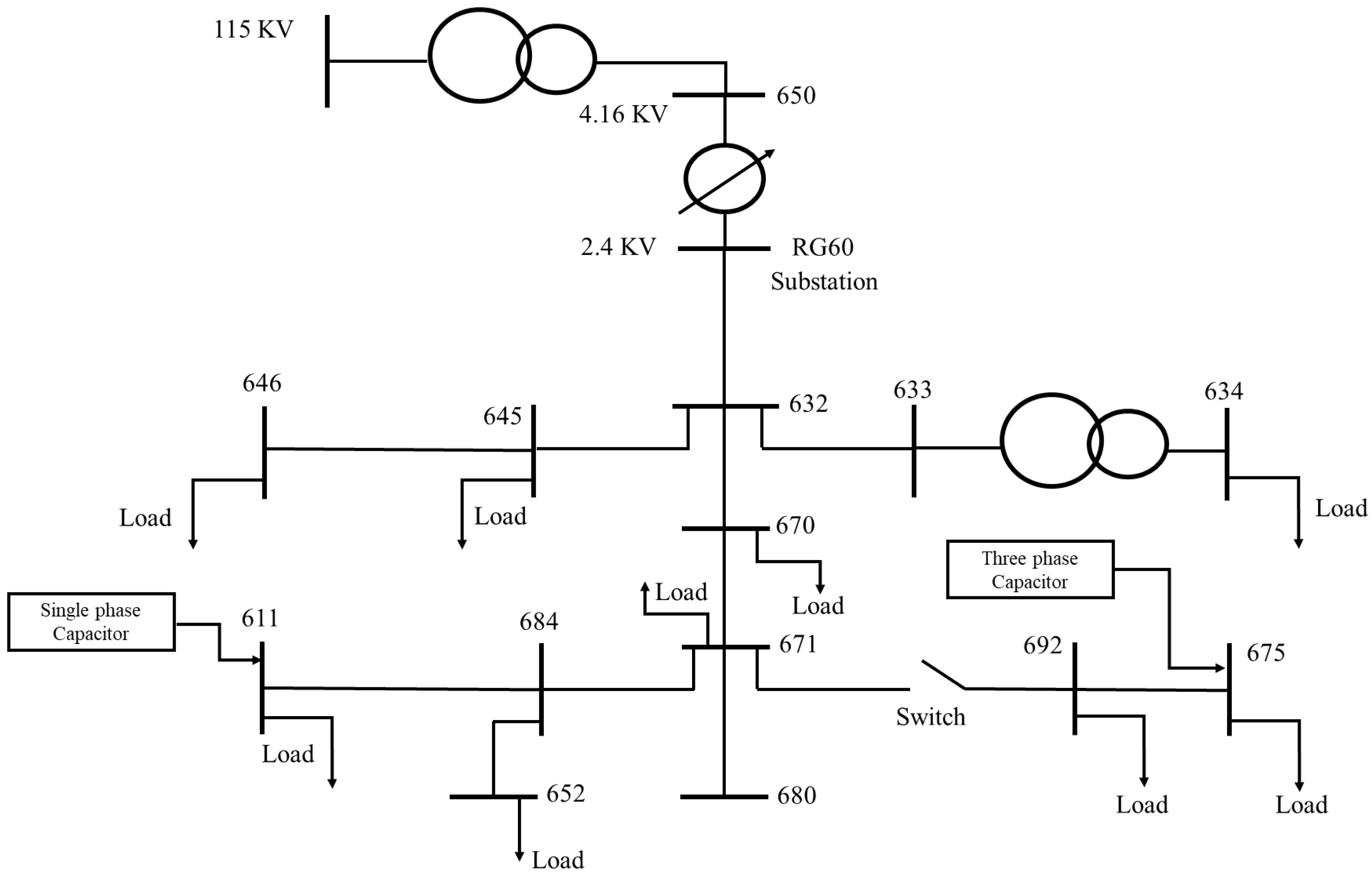
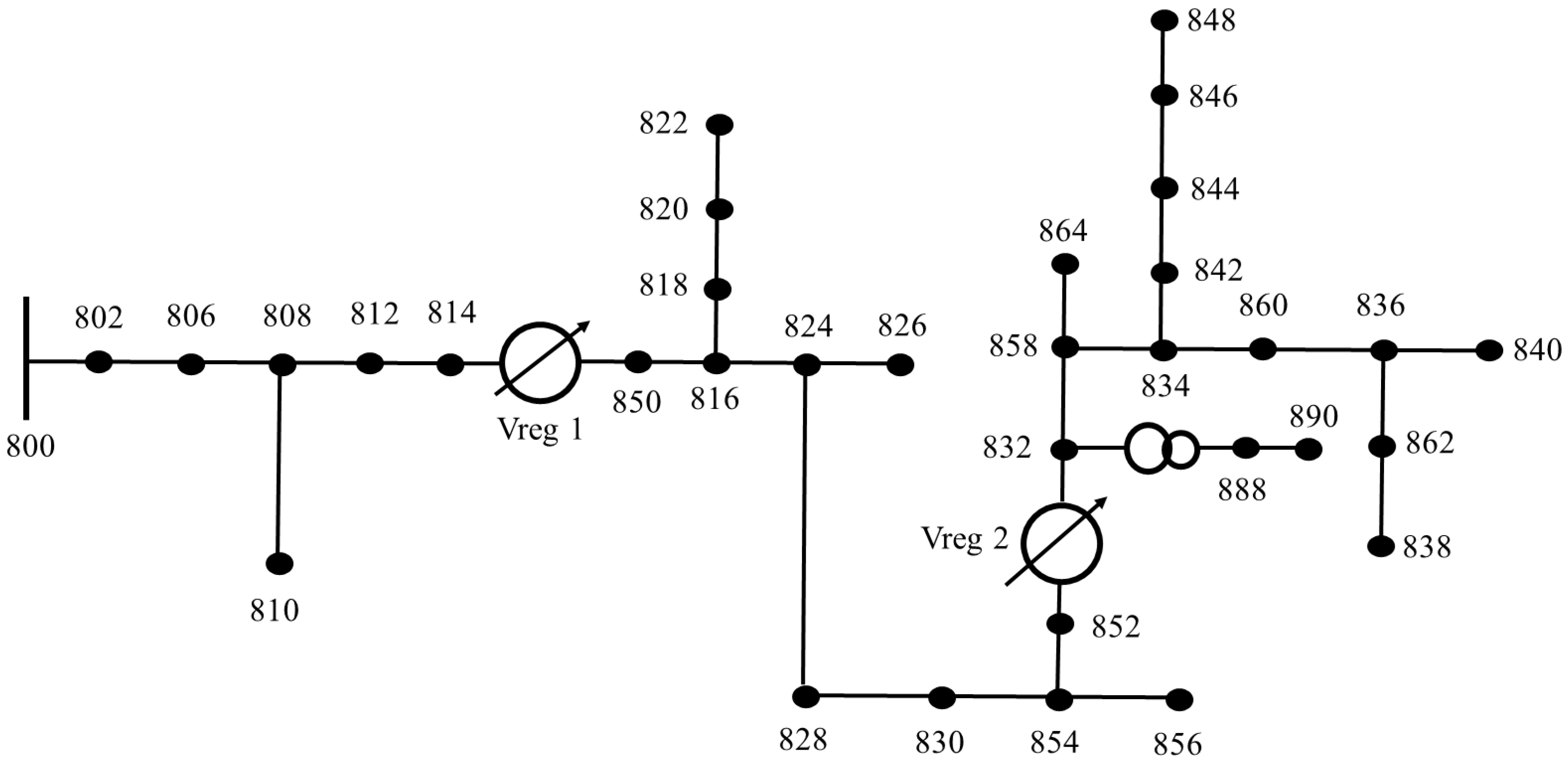
This section describes the CVR comparison study conducted for the IEEE-13 and IEEE-34 bus systems, using the feeder correlated comparison-based method. These two systems are shown in Figure 1 and Figure 2. Two feeders, i.e., feeder 1 and feeder 2, have been selected for CVR-off case and CVR-on case, respectively. The CVR-off case is the scenario when the CVR is not being implemented, i.e., we have selected a base voltage regulator setting for the system, whereas in the CVR-on case, the CVR is being implemented by reducing the base voltage regulator setting to different voltage levels. The voltage and power level between both the feeders have been compared to calculate the CVR factor. The CVR factor for active and reactive power has been calculated using the following formulas:

$$CVR factor for P=\frac{P_{off}-P_{on}}{P_{off}}/\frac{V_{off}-V_{on}}{V_{off}}$$

(1)

$$CVR factor for Q=\frac{Q_{off}-Q_{on}}{Q_{off}}/\frac{V_{off}-V_{on}}{V_{off}}$$

(2)

We have used the average voltage magnitude (V), total active power P and reactive power Q of all the phases in the calculation. The aforesaid quantities have been calculated as shown in the following equations:

$$\begin{gathered} Average voltage magnitude=\frac{V_A+V_B+V_C}{3} \\ where V_A, V_B and V_C are the voltages of phase A, B and C, respectively. \end{gathered}$$

(3)

$$\begin{gathered} Total Active Power=P_A+P_B+P_C \\ \mathit{where} P_A, P_B \mathit{and} P_C \mathit{are} \mathit{the} \mathit{active} \mathit{power} \mathit{of} \mathit{phase} A, B \mathit{and} C, \mathit{respectively}. \end{gathered}$$

(4)

$$\begin{gathered} Total Reactive Power=Q_A+Q_B+Q_C \\ \mathit{where} Q_A, Q_B \mathit{and} Q_C \mathit{are} \mathit{the} \mathit{reactive} \mathit{power} \mathit{of} \mathit{phase} A, B \mathit{and} C, \mathit{respectively}. \end{gathered}$$

(5)

The P, Q and V quantities for the 13-bus and 34-bus systems have been obtained from their model simulated in OpenDSS. For both the systems, the models have been simulated for different voltage levels. For the 13-bus system, simulation has been carried out for different voltage regulator settings levels. The voltage regulator setting of 124 V has been taken as the voltage in the CVR-off scenario, whereas for the CVR-on scenario, the voltage has been reduced to three different levels, i.e., 118 V, 120 V and 122 V. The CVR factor has been calculated for the three voltage levels, where $V_{off}$, $P_{off}$ and $Q_{off}$ are the input quantities obtained at the voltage regulator setting of 124 V, i.e., the CVR-off case. $V_{on}$, $P_{on}$ and $Q_{on}$ are the input quantities obtained for the voltage regulator settings considered in the CVR-on case.

In the 34-bus system, three cases have been considered, i.e., Case 1, Case 2 and Case 3. Case 1 is the scenario where the substation voltage is being varied when the voltage regulators are present in the system. In Case 2, the voltage regulators are disabled by replacing them with a short transmission line and then the substation voltage is varied. Case 3 involves proportional changes in the substation voltage and voltage regulator setting. In Case 1 and case 2, the substation voltage of 1.05 per unit (p.u.) has been considered as the voltage in the CVR-off case. For the CVR-on case, the substation voltages considered are 0.95, 1.00, 1.02 and 1.03 p.u. There are two voltage regulators in the 34-bus system whose settings are 122 V and 124 V, which remain the same in Case 1 and Case 2 for the CVR-off and CVR-on case. However, in Case 3, if the voltage from 1.05 p.u. is decreased to 1.02 p.u., then the voltage setting of both the regulators will change to (122 * (1.02/1.05)) V and (124 * (1.02/1.05)) V, respectively. This ratio will apply to other voltage settings as well. The only parameter that will vary in this ratio will be the substation voltages in the CVR-on case. These different scenarios intend to illustrate the impact of voltage regulator settings on CVR results.

For both the systems, eight ZIP load models have been considered in the study for all the loads of the 13-bus and 34-bus systems. The models considered are (0.2 0.2 0.6), (0.2 0.6 0.2), (0.6 0.2 0.2), (0.1 0.2 0.7), (0.7 0.1 0.2), (0 0 1), (0 1 0) and (1 0 0).

Two approaches were used to calculate the CVR factor for the 13-bus and 34-bus systems. The first approach involved utilizing the quantities of interest, i.e., P, Q and V from the input substation bus of the system. The second approach derived P and Q from the sum of all loads connected to the system, and the voltage was selected from the input bus of the system. The first approach will consider system losses and any reactive power compensating devices, as well as load characteristics, while the second approach specifically accounts for the characteristics of the loads themselves.

2.1. CVR Estimation Using Power Captured at Load

The IEEE-13 and IEEE-34 bus systems have 9 and 25 loads, respectively. For the second approach, the summation of P and Q of all the loads is taken as the input quantity and V is the input bus voltage at node RG60 for the 13-bus system. A similar approach for P and Q is followed for the 34-bus system and V is the input bus voltage at bus 800.

2.2. CVR Estimation Using Power Captured at Substation

In the IEEE 13-bus system, when using approach 1, P and Q are the power flow between bus RG60 and 632, and V is the voltage at bus RG60, as shown in Figure 1. For the IEEE-34 bus system, P and Q are the power flow between bus 800 and 802, and V is the voltage at bus 800, as shown in Figure 2.

3. Proposed New Method for Active Power Loss Estimation Based on Least Squares Method

When the voltage is lowered due to the CVR scheme, the system loss will usually be reduced together with the load. Calculating the respective value for the system loss reduction and load reduction is desirable. This section presents a new method to estimate the system loss based on substation voltage and substation active and reactive power input. This method uses two functions, i.e., Function 1 and Function 2, to calculate $P_{loss}^{estimated}$. The constants of the functions will be estimated using the least squares method. This approach was applied to both the 13-bus and 34-bus system.

3.1. Function 1

Function 1 for calculation of the power loss is given as

$$P_{loss}=\frac{K\left(P_1^2+Q_1^2\right)}{{\left|V_1\right|}^2}+C$$

(6)

where $K$ and $C$ are the constants.

The $P_{loss}$ is calculated for each hour over the span of 48 h. $P_1$, $Q_1$ and $V_1$ are the active power, reactive power, and input voltage, respectively, at the substation. All the three quantities are a column vector of order 48 by 1. The aforesaid constants are calculated using the following formula:

$$\left[\begin{array}{c}K\\ C\end{array}\right]={\left[H^{t}H\right]}^{-1}\left[H^{t}Z\right]$$

(7)

where

• $H=\left[\begin{array}{cc}a& j\end{array}\right]$
• $a=\frac{\left(P_1^2+Q_1^2\right)}{{\left|V_1\right|}^2} \mathrm{of} \mathrm{order} 48\times 1$
• $j={\left[1\right]}_{48\times 1}$
• $Z$: is the 48 × 1 $P_{loss}$.

3.2. Function 2

Function 2 for calculation of the power loss is given as

$$P_{loss}=\frac{K_1\left(P_1^2+Q_1^2\right)}{{\left|V_1\right|}^2}+\frac{K_2\sqrt{\left(P_1^2+Q_1^2\right)}}{\left|V_1\right|}+C$$

(8)

Function 2 is a quadratic equation, where $P_1$, $Q_1$ and $V_1$ are a column vector of order 48 × 1. The constants $K_1$, $K_2$ and $C$ are calculated using the following formula:

$$\left[\begin{array}{c}{K}_1\\ K_2\\ C\end{array}\right]={\left[H^{t}H\right]}^{-1}\left[H^{t}Z\right]$$

(9)

where

• $H=\left[\begin{array}{ccc}a& \sqrt{a}& j\end{array}\right]$
• $a=\frac{\left(P_1^2+Q_1^2\right)}{{\left|V_1\right|}^2} \mathrm{of} \mathrm{order} 48\times 1$
• $j={\left[1\right]}_{48\times 1}$.

After the constants of the functions are obtained, these two functions can be used to estimate the loss based on real time measurements of the voltage, real and reactive power at the substation. The power loss obtained from the functions is termed as “estimated power loss ($P_{loss}^{estimated}$)”. The power loss obtained from the model simulated in OpenDSS is called “simulated power loss ($P_{loss}^{simulated}$)”. The error in the power loss calculation for each hour has been calculated using the difference between $P_{loss}^{simulated}$ and $P_{loss}^{estimated}$. Using these error values, RMS error has been obtained for each ZIP load model and voltage setting. In addition to individually calculating the errors for each ZIP model and voltage setting, the errors have also been calculated by combining all the cases together. The total number of samples is 1152 (48 × 24) and 1920 (48 × 40) for the 13-bus and 34-bus systems, respectively. In the 13-bus system, 24 is the total number of voltage settings, i.e., 3 multiplied by the total number of ZIP models, i.e., 8. In the 34-bus system, 40 is the total number of substation voltage levels, i.e., 5 multiplied by the total number of ZIP models, i.e., 8. Forty-eight is the total number of hours in each case.

4. Proposed New Method for Active Power Loss Estimation Based on ANN Method

This section describes the proposed new ANN-based active power loss estimation method. This method uses feedforward neural network models with one, two or three hidden layers. As an example, Figure 3 illustrates a two hidden layer ANN. These models take $P_1$, $Q_1$ and $V_1$ as inputs and $P_{loss}$ as the target data to train the network. The input quantities are taken from the substation measurement values. The $P_{loss}^{simulated}$ is the loss obtained in simulation and is calculated as the difference between the active power obtained at the substation and load. The feedforward model follows supervised learning training using the input quantities and the simulated loss quantities. Once the network is trained, supplying inputs will lead to estimated loss $P_{loss}^{estimated}$. The difference between $P_{loss}^{estimated}$ and $P_{loss}^{simulated}$ has been used to calculate the RMS value for the 13-bus and 34-bus systems.

The hidden layers shown in Figure 3 contain 10 neurons. The output layer contains only one neuron. The number of neurons in the hidden layer(s) of the above models have been varied from 5 to 16 and $P_{loss}$ has been obtained for each case. The aforesaid variation has been carried out to study the effect of number of neurons and hidden layers on loss estimation accuracy. The variables $P_1$, $Q_1$, $V_1$ and $P_{loss}$ are a matrix combining the respective data for all the cases for all the ZIP load models.

5. Case Studies

Section 5 presents the results obtained for the CVR comparison study using the approaches discussed in Section 2. It also discusses the loss relationship study performed using the function and ANN method discussed in Section 4.

5.1. CVR Studies

The CVR factors for both 13-bus and 34 bus systems are highest when the impedance component is high in the ZIP load, being the highest in the case of the constant impedance load. This is consistent with the theoretical CVR factor being 2.0, 1.0 and 0 for the constant impedance load, constant current load and constant power load, respectively.

For the 34-bus system, a voltage regulator plays a crucial role in CVR factor calculation. In case 1, i.e., when the voltage regulators are enabled, the CVR factor for P is quite low and even negative in some cases. This is due to the restriction in the change in voltage, as both the voltage regulators are only permitted to vary the voltage within the specified bandwidth. In case 2, when we disable the voltage regulators by replacing them with a short transmission line, it can be observed that the CVR factor increases. In case 3, where we vary the voltage regulator setting and substation voltage level in a proportionate manner, it can be observed that the CVR factor increases to a level consistent with the load characteristics.

Analysis of the CVR factor for reactive power is more complicated. When CVR for Q is calculated using the sum of load reactive power consumption, the value is consistent with the load characteristics. However, when the CVR for Q is calculated using the measurements at the substation, i.e., RG60 in the 13-bus system and bus 800 in the 34-bus system, the measurements reflect not only the load characteristics but also the capacitor compensation.

The following sections show the average CVR factor calculated for both the systems for all the eight ZIP load models over the duration of 48 h.

5.1.1. IEEE-13 Bus System

Table 1. Average CVR factor obtained using power captured at loads.

ZIP Load	Average CVR Factor for P			Average CVR Factor for Q
	118 V	120 V	122 V	118 V	120 V	122 V
(0.2 0.6 0.2)	1.06	1.06	1.06	1.06	1.06	1.06
(0.2 0.2 0.6)	0.65	0.66	0.66	0.65	0.66	0.66
(0.6 0.2 0.2)	1.39	1.37	1.29	1.39	1.37	1.30
(0.1 0.2 0.7)	0.44	0.45	0.45	0.44	0.45	0.45
(0.7 0.1 0.2)	1.52	1.53	1.54	1.52	1.53	1.54
(0 0 1)	0.00	0.00	0.00	0.00	0.00	0.00
(0 1 0)	1.06	1.07	1.06	1.06	1.06	1.06
(1 0 0)	1.96	1.97	1.98	1.96	1.97	1.98

and

Table 2. Average CVR factor obtained using power captured at substation.

ZIP Load	Average CVR Factor for P			Average CVR Factor for Q
	118 V	120 V	122 V	118 V	120 V	122 V
(0.2 0.6 0.2)	1.03	1.04	1.03	0.21	0.20	0.20
(0.2 0.2 0.6)	0.61	0.62	0.62	−0.60	−0.60	−0.60
(0.6 0.2 0.2)	1.42	1.43	1.43	0.94	0.96	0.95
(0.1 0.2 0.7)	0.39	0.40	0.40	−1.02	−1.03	−1.02
(0.7 0.1 0.2)	1.51	1.52	1.53	1.12	1.13	1.13
(0 0 1)	−0.07	−0.07	−0.06	−1.93	−1.93	−1.92
(0 1 0)	1.04	1.04	1.03	0.22	0.21	0.19
(1 0 0)	1.96	1.97	1.98	1.96	1.97	1.98

show the average CVR factor for the IEEE-13 bus system obtained by using the power captured at the loads and substation, respectively.

Table 1 clearly reveals that the CVR factors calculated using the power measurements at the load location reflect the load characteristics. In contrast, it can be observed from Table 2 that some CVR values for Q are negative due to capacitor bank compensation. When the substation voltage reduces, the load reactive power reduces, but the reactive power injection from the capacitor bank also reduces and in addition, the reactive power loss on the lines increases, so the reactive power input at the substation increases, leading to a negative CVR value for Q. A numerical example is provided below.

If one takes one hour power flow as an example, in the base case with 124 V, the reactive power from RG60 to 632 is 677.87 kVar. The total load reactive power consumption is 1298.74 kVar. The capacitor bank reactive power injection is 730.02 kVar. The line reactive power loss is 109.15 kVar. In the case with 118 V, the reactive power from RG60 to 632 is 715.41 kVar. The total load reactive power consumption is 1260.27 kVar. The capacitor bank reactive power injection is 659.85 kVar. The line reactive power loss is 114.99 kVar. The CVR for Q calculated using load measurements would be 0.61, while the value calculated using substation measurements would be −1.14.

5.1.2. IEEE-34 Bus System

Table 3. Average CVR factor obtained using power captured at load for case 1.

ZIP Load	Average CVR Factor for P				Average CVR Factor for Q
	0.95	1	1.02	1.03	0.95	1	1.02	1.03
(0.2 0.6 0.2)	0.88	0.83	0.83	0.83	0.93	0.87	0.87	0.87
(0.2 0.2 0.6)	0.62	0.51	0.50	0.50	0.66	0.53	0.53	0.53
(0.6 0.2 0.2)	1.12	1.11	1.11	1.11	1.18	1.16	1.17	1.17
(0.1 0.2 0.7)	0.51	0.35	0.34	0.34	0.54	0.37	0.36	0.36
(0.7 0.1 0.2)	1.19	1.18	1.18	1.18	1.24	1.24	1.24	1.24
(0 0 1)	0.30	0.04	0.01	0.00	0.33	0.05	0.01	0.00
(0 1 0)	0.91	0.85	0.84	0.84	0.95	0.89	0.89	0.89
(1 0 0)	1.53	1.53	1.53	1.53	1.59	1.60	1.61	1.61

and

Table 4. Average CVR factor using power captured at substation for case 1.

ZIP Load	Average CVR Factor for P				Average CVR Factor for Q
	0.95	1	1.02	1.03	0.95	1	1.02	1.03
(0.2 0.6 0.2)	0.14	−0.04	−0.09	−0.09	−3.56	−2.87	−3.73	−4.76
(0.2 0.2 0.6)	0.02	−0.07	−0.10	−0.10	6.68	4.53	4.83	5.74
(0.6 0.2 0.2)	0.26	0.01	−0.08	−0.08	−3.39	−2.59	−3.09	−3.28
(0.1 0.2 0.7)	−0.05	−0.09	−0.11	−0.10	3.47	2.36	2.52	2.80
(0.7 0.1 0.2)	0.28	0.02	−0.09	−0.10	−0.89	−0.52	−1.06	−1.20
(0 0 1)	−0.20	−0.15	−0.13	−0.12	−0.75	−0.13	0.32	0.26
(0 1 0)	0.15	−0.04	−0.09	−0.09	−6.91	−5.27	−6.29	−8.27
(1 0 0)	0.39	0.05	−0.09	−0.09	2.22	2.49	2.53	2.74

show the average CVR factor obtained for case 1 using both the CVR calculation approaches discussed in Section 2.

Table 5. Average CVR factor obtained using power captured at load for case 2.

ZIP Load	Average CVR Factor for P				Average CVR Factor for Q
	0.95	1	1.02	1.03	0.95	1	1.02	1.03
(0.2 0.6 0.2)	0.25	0.09	0.05	0.04	0.24	0.09	0.04	0.03
(0.2 0.2 0.6)	0.16	0.06	0.03	0.03	0.15	0.05	0.03	0.02
(0.6 0.2 0.2)	0.33	0.13	0.06	0.05	0.32	0.12	0.05	0.04
(0.1 0.2 0.7)	0.11	0.04	0.02	0.02	0.11	0.04	0.02	0.02
(0.7 0.1 0.2)	0.35	0.14	0.06	0.04	0.34	0.13	0.05	0.03
(0 0 1)	0.00	0.00	0.00	0.00	0.00	0.00	0.00	0.00
(0 1 0)	0.25	0.09	0.05	0.04	0.24	0.08	0.04	0.03
(1 0 0)	0.44	0.18	0.07	0.06	0.43	0.16	0.05	0.04

and

Table 6. Average CVR factor using power captured at substation for case 2.

ZIP Load	Average CVR Factor for P				Average CVR Factor for Q
	0.95	1	1.02	1.03	0.95	1	1.02	1.03
(0.2 0.6 0.2)	1.29	1.21	1.18	1.16	21.52	25.21	28.48	29.66
(0.2 0.2 0.6)	1.05	0.90	0.85	0.82	−6.63	−8.16	−9.01	−9.97
(0.6 0.2 0.2)	1.51	1.49	1.48	1.48	3.94	4.45	4.65	4.63
(0.1 0.2 0.7)	0.96	0.76	0.70	0.67	1.20	0.90	1.43	1.34
(0.7 0.1 0.2)	1.57	1.56	1.56	1.56	−0.60	−0.90	−1.30	−1.55
(0 0 1)	0.79	0.48	0.40	0.37	7.86	8.41	9.94	11.24
(0 1 0)	1.31	1.23	1.20	1.18	3.57	4.00	4.38	4.36
(1 0 0)	1.91	1.95	1.97	1.98	1.91	1.95	1.97	1.98

show the average CVR factor obtained for case 2 using the aforesaid methods.

Table 7. Average CVR factor obtained using power captured at load for case 3.

ZIP Load	Average CVR Factor for P				Average CVR Factor for Q
	0.95	1	1.02	1.03	0.95	1	1.02	1.03
(0.2 0.6 0.2)	0.78	0.77	0.78	0.76	0.82	0.81	0.82	0.81
(0.2 0.2 0.6)	0.46	0.46	0.47	0.47	0.48	0.49	0.49	0.50
(0.6 0.2 0.2)	1.07	1.08	1.08	1.08	1.12	1.14	1.14	1.14
(0.1 0.2 0.7)	0.31	0.31	0.31	0.31	0.33	0.32	0.33	0.33
(0.7 0.1 0.2)	1.15	1.16	1.16	1.15	1.20	1.22	1.22	1.21
(0 0 1)	0.00	0.00	0.00	0.00	0.00	0.00	0.00	0.00
(0 1 0)	0.78	0.77	0.77	0.76	0.82	0.81	0.81	0.80
(1 0 0)	1.52	1.53	1.53	1.53	1.59	1.60	1.60	1.61

and

Table 8. Average CVR factor using power captured at substation for case 3.

ZIP Load	Average CVR Factor for P				Average CVR Factor for Q
	0.95	1	1.02	1.03	0.95	1	1.02	1.03
(0.2 0.6 0.2)	0.94	0.91	0.93	0.92	−5.40	−6.54	−7.36	−10.50
(0.2 0.2 0.6)	0.49	0.44	0.46	0.47	24.06	24.77	26.15	24.72
(0.6 0.2 0.2)	1.31	1.35	1.36	1.37	−5.70	−5.67	−5.99	−5.53
(0.1 0.2 0.7)	0.28	0.21	0.22	0.23	16.23	17.28	17.91	18.16
(0.7 0.1 0.2)	1.42	1.46	1.47	1.46	−0.29	−0.37	−0.31	−0.21
(0 0 1)	−0.14	−0.28	−0.27	−0.26	6.93	6.25	7.32	8.06
(0 1 0)	0.94	0.92	0.93	0.92	−14.09	−16.07	−17.13	−21.26
(1 0 0)	1.91	1.96	1.98	1.99	1.93	2.01	2.06	2.11

show the results for case 3.

5.2. Active Power Loss Estimation Using Least Squares Method

There is no direct relationship between active power loss and CVR factor. The active power loss is obtained as a function of substation voltage and, active and reactive power inputs. This section presents the active power loss estimation using the least squares method for the IEEE-13 and 34 bus system. For both the systems, the value of $P_{loss}^{estimated}$ obtained using curve fitting approach is very similar to $P_{loss}^{simulated}$, which can be observed in the following figures.

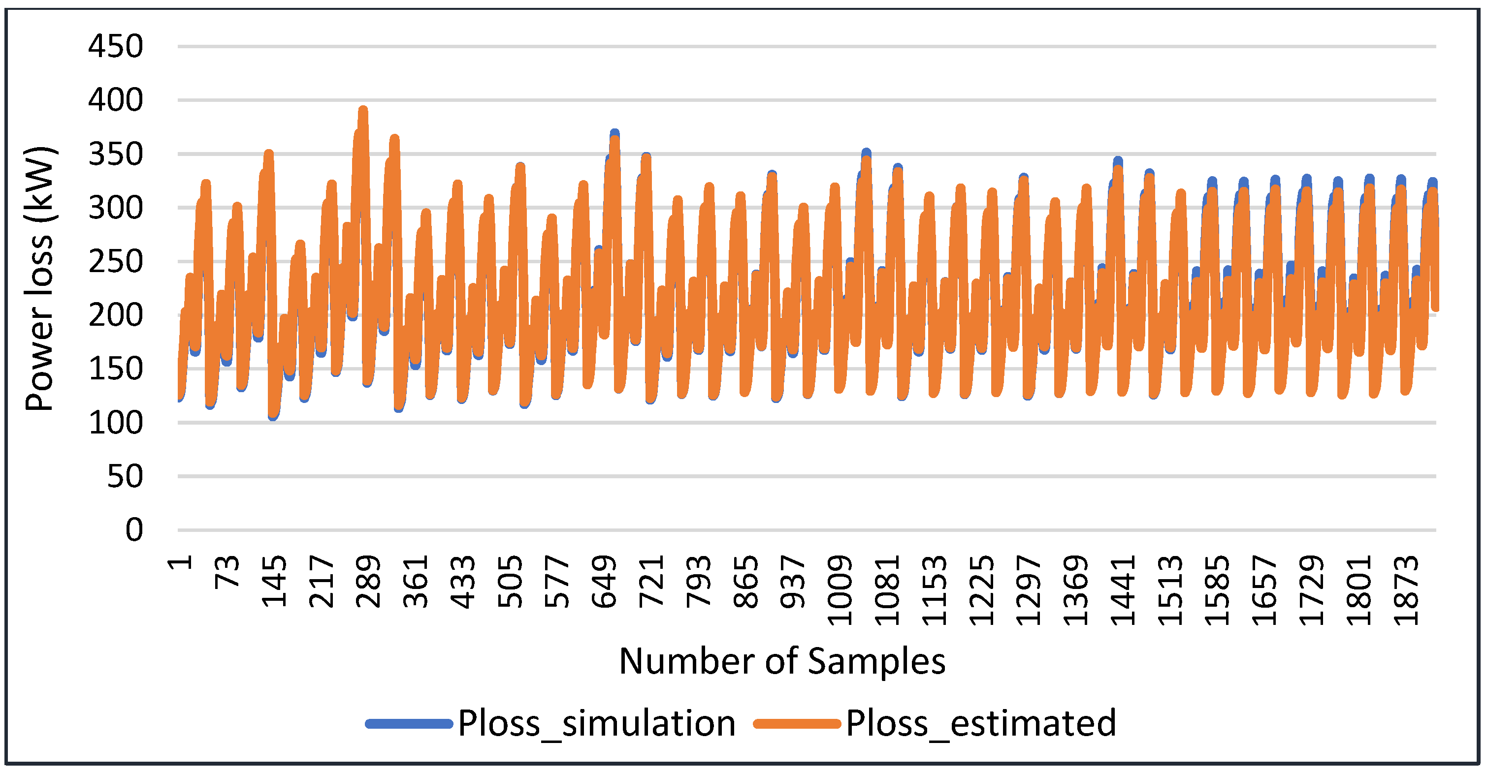
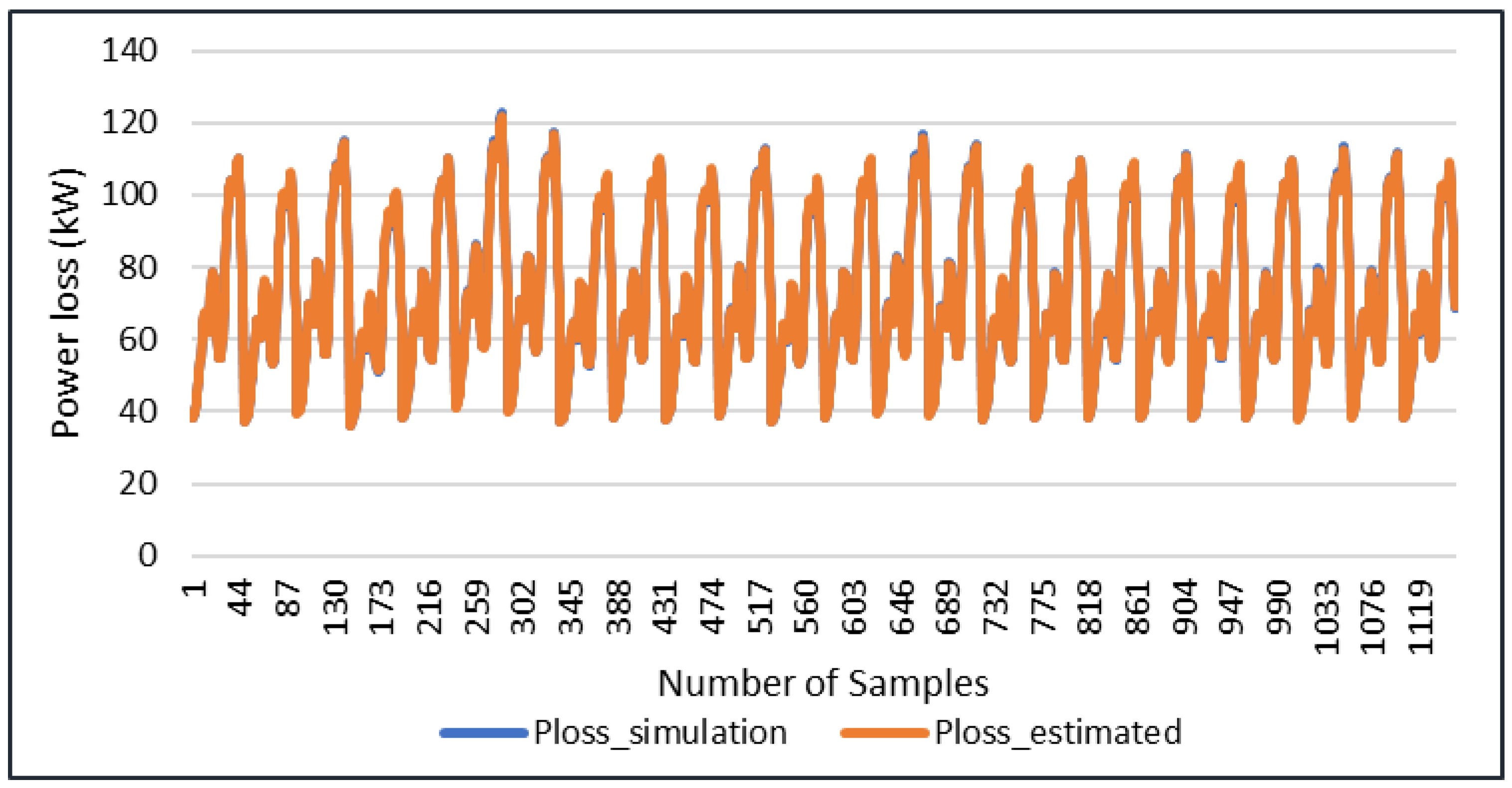
5.2.1. IEEE-13 Bus System

For the IEEE-13 bus system, the coefficients for function 1 were obtained as $K=45.1501 \mathrm{and} C=-0.076$. The coefficients for function 2 were $K_1=44.1627, K_2=1.2666 \mathrm{and} C=-0.0018$.

Figure 4 and Figure 5 depict the active power loss estimation obtained from function 1 and 2, respectively.

In the 13-bus system, it can be observed from the graphs that the estimated power loss obtained from both functions is very close to the simulated power loss obtained from OpenDSS. The RMS error obtained using function 2 (0.47 kW) was lower than function 1 (0.53 kW). This was true for combined cases, where all ZIP cases are combined, as well as for individual cases, where each ZIP case is dealt with individually.

Table 9. RMS error for active power loss estimation for function 1 and 2 for IEEE-13 bus system.

ZIP Parameter	Voltage Setting	Function 1	Function 2
(0.2 0.6 0.2)	118 V	0.31	0.08
	120 V	0.30	0.08
	122 V	0.33	0.09
(0.6 0.2 0.2)	118 V	0.34	0.06
	120 V	0.35	0.06
	122 V	0.36	0.07
(0.2 0.2 0.6)	118 V	0.28	0.10
	120 V	0.26	0.10
	122 V	0.31	0.11
(0.1 0.2 0.7)	118 V	0.82	0.41
	120 V	0.83	0.47
	122 V	0.88	0.41
(0.7 0.1 0.2)	118 V	0.89	0.44
	120 V	0.91	0.42
	122 V	0.88	0.41
(1 0 0)	118 V	0.38	0.04
	120 V	0.40	0.04
	122 V	0.41	0.06
(0 1 0)	118 V	0.31	0.08
	120 V	0.30	0.08
	122 V	0.33	0.09
(0 0 1)	118 V	0.21	0.13
	120 V	0.19	0.13
	122 V	0.24	0.09

presents the RMS error in kW for active power loss estimation for function 1 and 2 for each ZIP case.

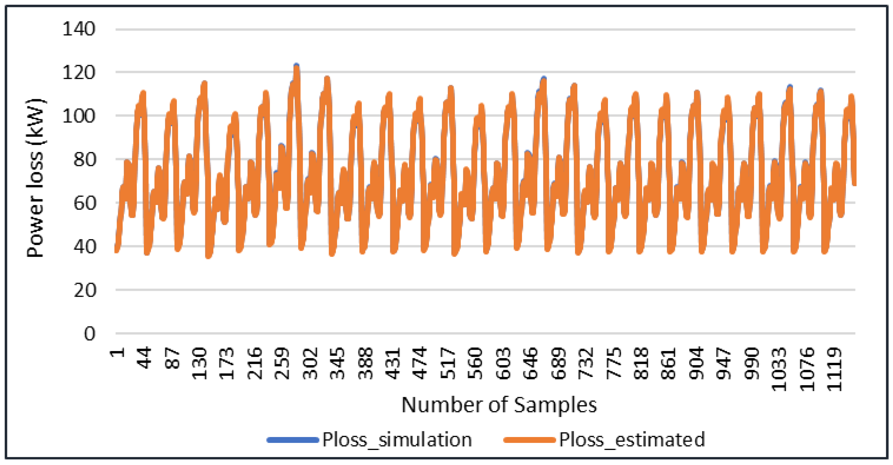
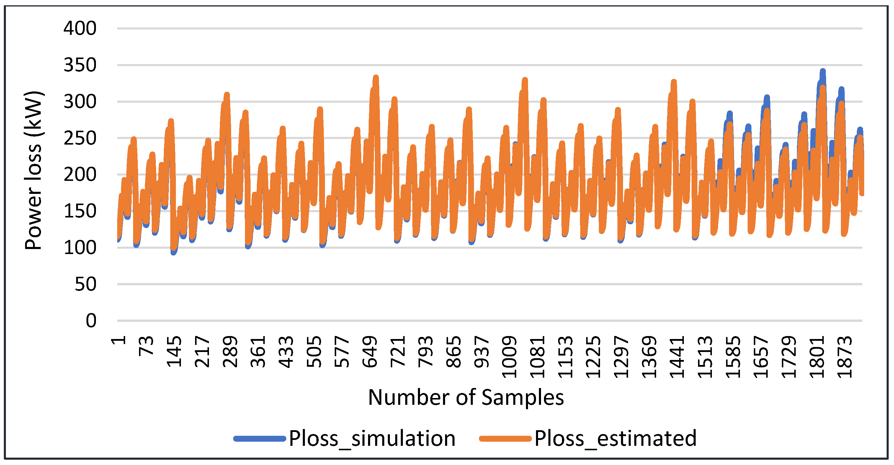
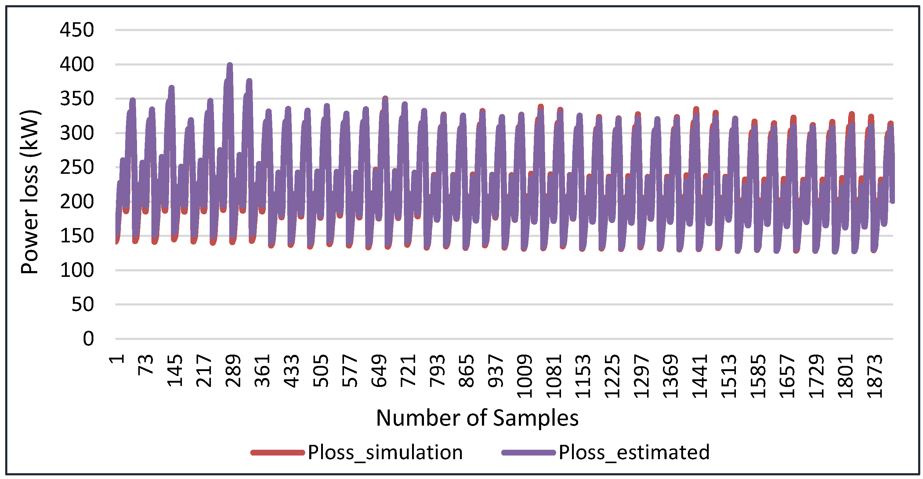
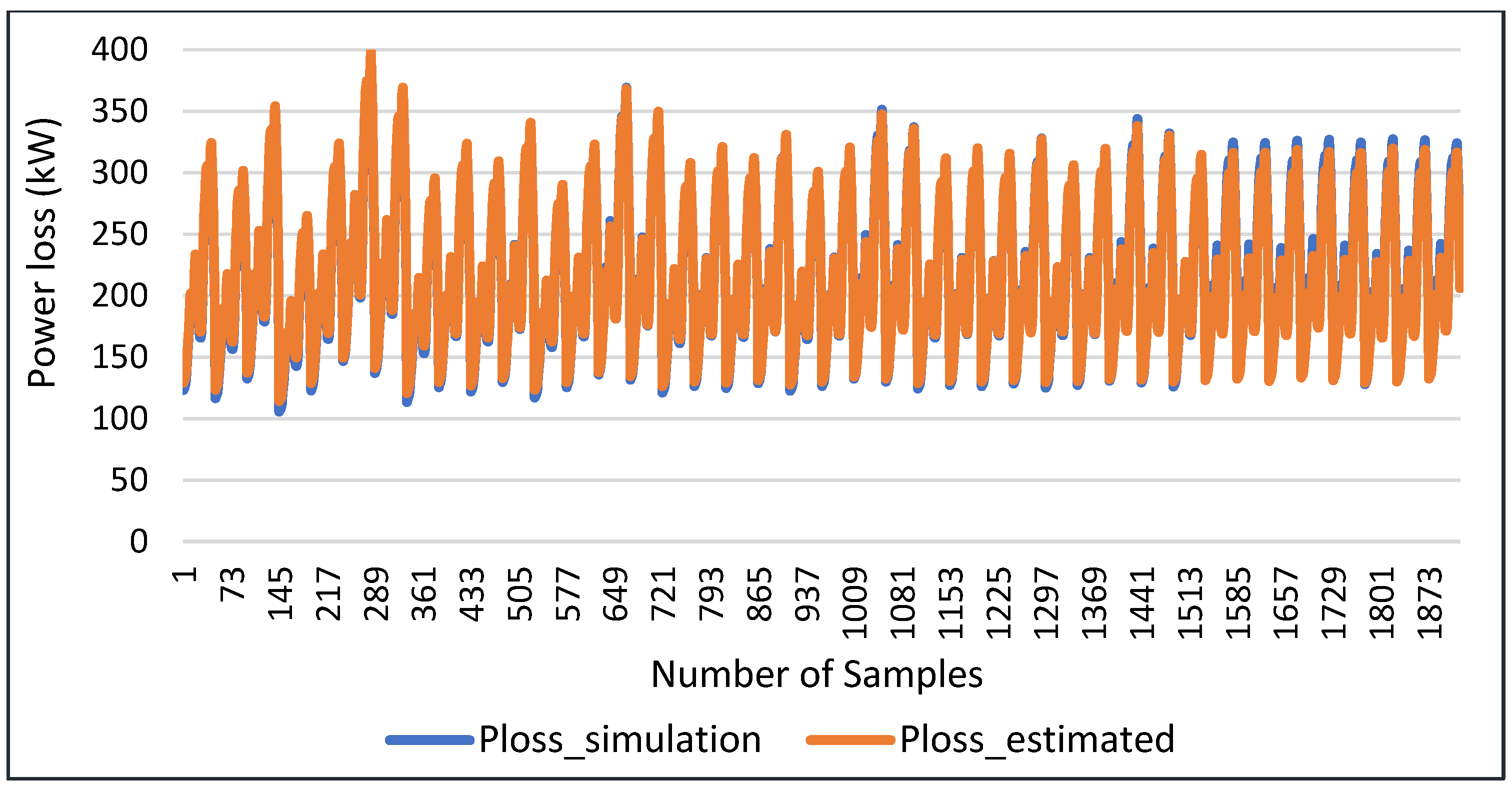
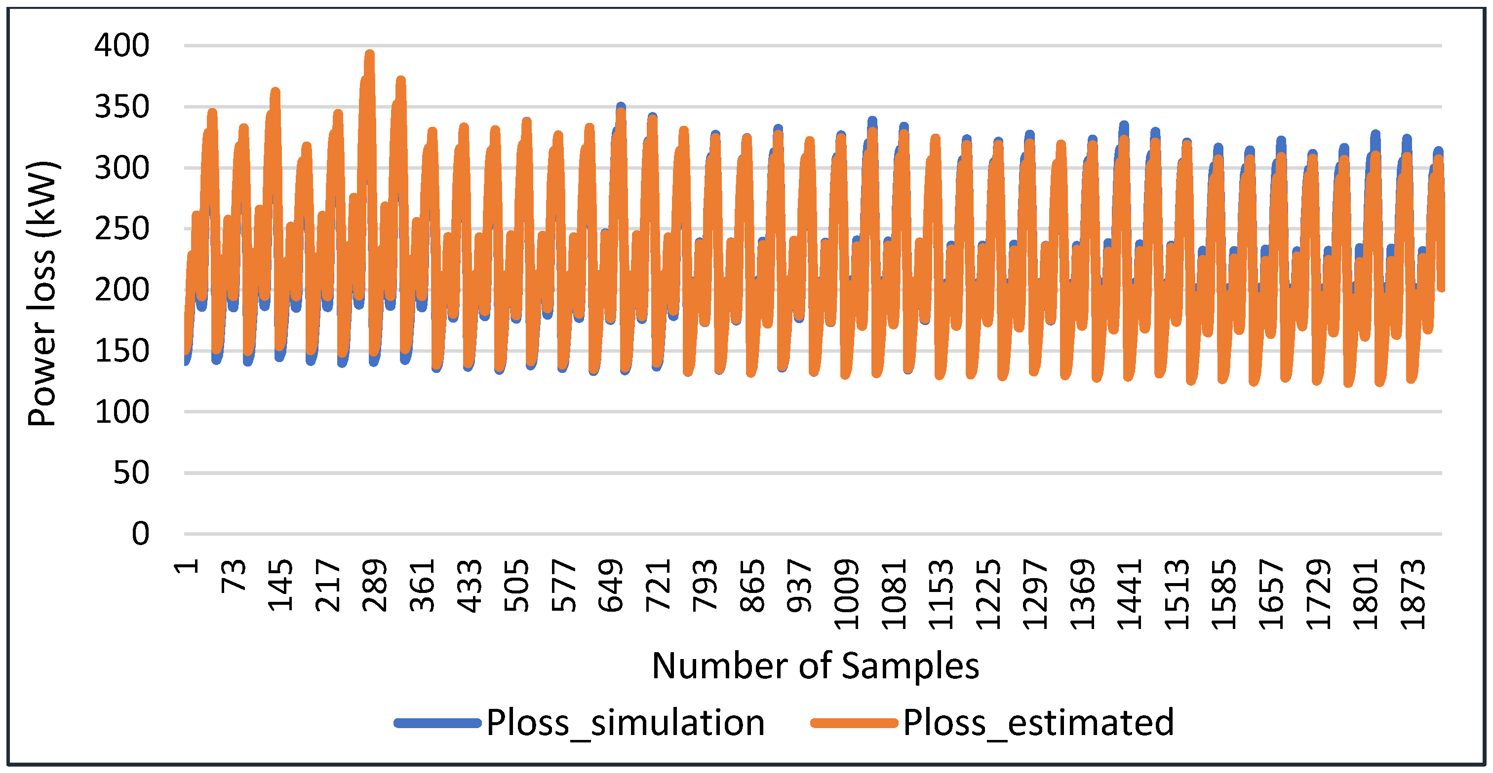
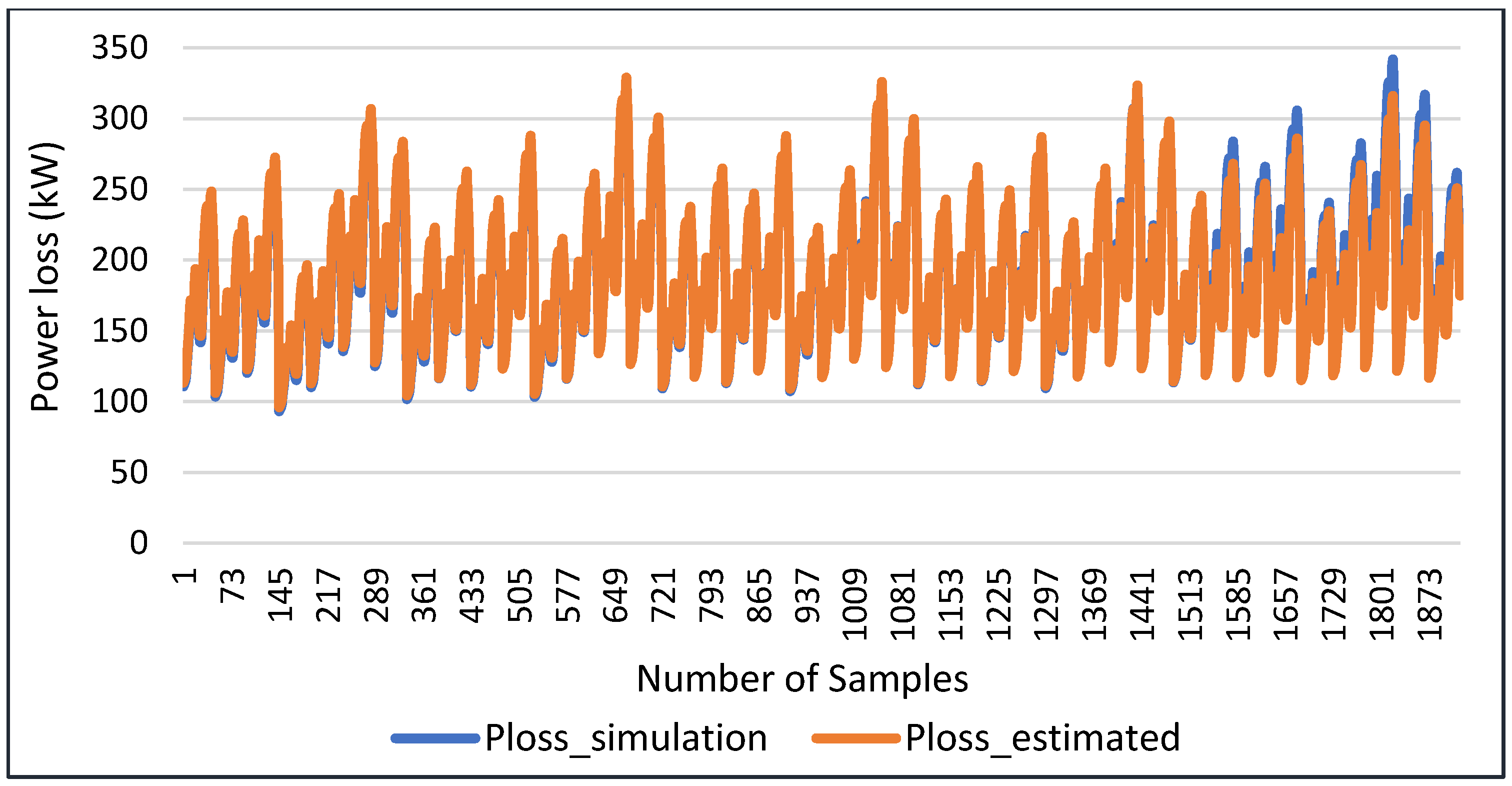
5.2.2. IEEE-34 Bus System

Figure 6, Figure 7, Figure 8, Figure 9, Figure 10 and Figure 11 depict the power loss obtained after calculating the constants for function 1 and 2, respectively, for all three cases by combining all the voltage levels and ZIP load models in a single matrix. The difference between $P_{loss}^{simulated}$ and $P_{loss}^{estimated}$ provides the RMS error for function 1 and function 2. The RMS error obtained for the aforesaid cases indicate function 2 as the most efficient relationship between power loss and substation voltage, active and reactive power, because of its low RMS error in comparison to function 1.

Function 1

For the IEEE-34 bus system, the coefficients for function 1 were obtained as $K=\mathrm{15,043} \mathrm{and} C=32$ for case 1, $K=\mathrm{16,874} \mathrm{and} C=21$ for case 2 and, $K=\mathrm{15,593} \mathrm{and} C=31$ for case 3. The RMS error is 5.80 kW for case 1, 7.78 kW for case 2 and 5.31 kW for case 3.

Table 10. RMS error for active power loss estimation for function 1 for IEEE-34 bus system.

ZIP Parameter	Voltage Setting	Case 1	Case 2	Case 3
(0.2 0.6 0.2)	0.95	0.79	0.78	1.35
	1.00	1.01	0.93	1.28
	1.02	1.04	1.11	1.24
	1.03	1.18	1.15	1.28
(0.6 0.2 0.2)	0.95	0.79	0.69	1.25
	1.00	1.00	0.86	1.21
	1.02	1.03	0.90	1.27
	1.03	1.18	0.90	1.33
(0.2 0.2 0.6)	0.95	0.79	0.72	1.49
	1.00	0.96	1.03	1.33
	1.02	1.05	1.38	1.29
	1.03	1.16	1.48	1.32
(0.1 0.2 0.7)	0.95	0.82	0.70	1.48
	1.00	0.95	1.06	1.36
	1.02	1.08	1.45	1.31
	1.03	1.14	1.62	1.30
(0.7 0.1 0.2)	0.95	0.79	0.67	1.20
	1.00	1.00	0.83	1.17
	1.02	1.02	0.84	1.29
	1.03	1.18	0.84	1.33
(1 0 0)	0.95	0.77	0.55	1.12
	1.00	0.97	0.57	1.21
	1.02	1.03	0.60	1.23
	1.03	1.15	0.61	1.25
(0 1 0)	0.95	0.82	0.76	1.39
	1.00	1.01	0.92	1.28
	1.02	1.04	1.09	1.24
	1.03	1.17	1.13	1.28
(0 0 1)	0.95	1.00	0.59	1.57
	1.00	0.97	1.24	1.45
	1.02	1.06	1.55	1.40
	1.03	1.13	1.85	1.28

presents the RMS error for active power loss estimation for function 1 for each ZIP case.

Function 2

For the IEEE-34 bus system, the coefficients for function 2 were obtained as $K_1=\mathrm{11,218}, K_2=872 \mathrm{and} C=-17$ for case 1, $K_1=\mathrm{12,838}, K_2=818 \mathrm{and} C=-19$ for case 2 and, $K_1=\mathrm{10,680}, K_2=1087 \mathrm{and} C=-28$ for case 3. The RMS error is 5.69 kW for case 1, 7.73 kW for case 2 and 5.09 kW for case 3.

Table 11. RMS error for active power loss estimation for function 2 for IEEE-34 bus system.

ZIP Parameter	Voltage Setting	Case 1	Case 2	Case 3
(0.2 0.6 0.2)	0.95	0.12	0.12	0.51
	1.00	0.37	0.11	0.55
	1.02	0.45	0.08	0.50
	1.03	0.48	0.06	0.52
(0.6 0.2 0.2)	0.95	0.09	0.07	0.54
	1.00	0.40	0.10	0.51
	1.02	0.44	0.04	0.51
	1.03	0.51	0.03	0.56
(0.2 0.2 0.6)	0.95	0.15	0.16	0.47
	1.00	0.37	0.11	0.55
	1.02	0.45	0.16	0.53
	1.03	0.47	0.12	0.55
(0.1 0.2 0.7)	0.95	0.18	0.16	0.44
	1.00	0.37	0.12	0.59
	1.02	0.46	0.20	0.52
	1.03	0.45	0.14	0.52
(0.7 0.1 0.2)	0.95	0.09	0.07	0.49
	1.00	0.40	0.07	0.49
	1.02	0.45	0.03	0.53
	1.03	0.51	0.03	0.57
(1 0 0)	0.95	0.07	0.12	0.46
	1.00	0.36	0.03	0.49
	1.02	0.44	0.04	0.51
	1.03	0.52	0.04	0.52
(0 1 0)	0.95	0.12	0.13	0.51
	1.00	0.36	0.10	0.51
	1.02	0.45	0.07	0.50
	1.03	0.48	0.06	0.51
(0 0 1)	0.95	0.28	0.11	0.42
	1.00	0.41	0.13	0.61
	1.02	0.47	0.22	0.53
	1.03	0.45	0.25	0.48

presents the RMS error for active power loss estimation for function 2 for each ZIP case.

It is noted that the RMS error for the combined cases is generally larger than that for each ZIP case. In practical applications, the ZIP parameters can be estimated using feeder head measurements including voltage and power. Then, the function coefficients can be estimated using that specific ZIP case for more accurate active power loss estimation.

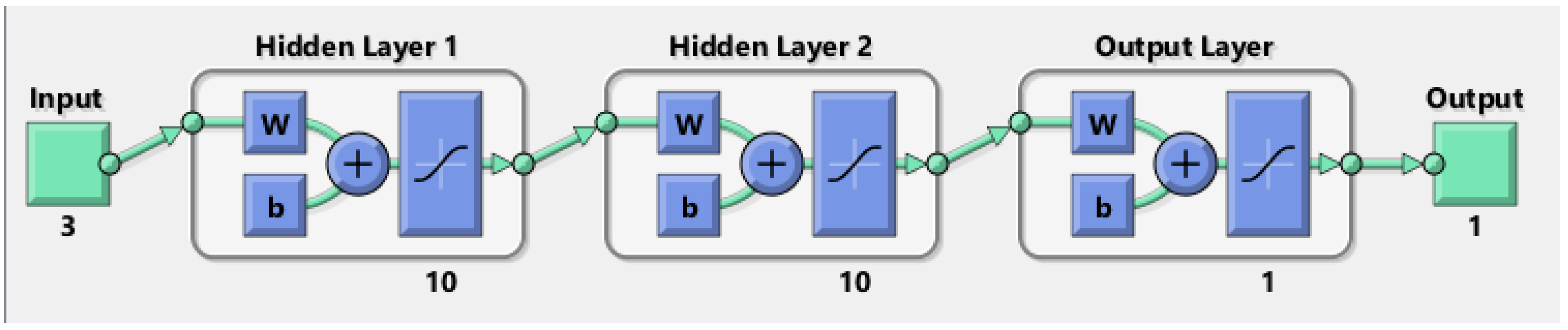
5.3. Active Power Loss Estimation Using ANN Method

Table 12. RMS error for active power loss estimation for IEEE-13 bus system.

RMS Error		Number of Neurons in Hidden Layer
		5	6	7	8	9	10	11	12	13	14	15	16
Number of hidden layers	1	0.4806	0.4807	0.4808	0.4808	0.4808	0.4809	0.4808	0.4808	0.4808	0.4808	0.4808	0.4807
	2	0.4807	0.4807	0.4807	0.4809	0.4807	0.4808	0.4808	0.4808	0.4808	0.4808	0.4808	0.4812
	3	0.4808	0.4808	0.4808	0.4808	0.4808	0.4808	0.4808	0.4808	0.4808	0.4808	0.4812	0.4808

show the RMS error for loss estimation versus the number of neurons in the hidden layer for a given number of hidden layers for the IEEE-13 bus system.

Table 13. RMS error for active power loss estimation for IEEE-34 bus system (case 1).

RMS Error		Number of Neurons in Hidden Layer
		5	6	7	8	9	10	11	12	13	14	15	16
Number of hidden layers	1	5.6860	5.6861	5.6873	5.6875	5.6876	5.6877	5.6873	5.6872	5.6872	5.6874	5.6872	5.6873
	2	5.6872	5.6869	5.6873	5.6874	5.6872	5.6872	5.6872	5.6872	5.6872	5.6872	5.6872	5.6872
	3	5.6873	5.6873	5.6871	5.6869	5.6872	5.6872	5.6878	5.6872	5.6872	5.6872	5.6872	5.6872

,

Table 14. RMS error for active power loss estimation for IEEE-34 bus system (case 2).

RMS Error		Number of Neurons in Hidden Layer
		5	6	7	8	9	10	11	12	13	14	15	16
Number of hidden layers	1	7.7288	7.7314	7.7298	7.7295	7.7298	7.7298	7.7298	7.7298	7.7299	7.7298	7.7298	7.7298
	2	7.7297	7.7299	7.7297	7.7298	7.7297	7.7298	7.7298	7.7298	7.7298	7.7298	7.7298	7.7298
	3	7.7299	7.8642	7.7298	7.7297	7.7298	7.7298	7.7301	7.7298	7.7299	7.7299	7.7298	7.7298

and

Table 15. RMS error for active power loss estimation for IEEE-34 bus system (case 3).

RMS Error		Number of Neurons in Hidden Layer
		5	6	7	8	9	10	11	12	13	14	15	16
Number of hidden layers	1	5.6860	5.6861	5.6873	5.6875	5.6876	5.6877	5.6873	5.6872	5.6872	5.6874	5.6872	5.6873
	2	5.6872	5.6869	5.6873	5.6874	5.6872	5.6872	5.6872	5.6872	5.6872	5.6872	5.6872	5.6872
	3	5.6873	5.6873	5.6871	5.6867	5.6872	5.6872	5.6878	5.6872	5.6872	5.6872	5.6872	5.6872

list the RMS error for loss estimation for the IEEE-34 bus system for case 1, 2 and 3, respectively.

The results indicate that the number of neurons and number of hidden layers do not have a substantial effect on the estimation accuracy. Thus, for simplicity, one hidden layer network with five neurons in the hidden layer will suffice.

6. Conclusions

This paper presents new insights about CVR factor calculation and factors affecting CVR implementation. This paper also proposes two new methods, a curve fitting method and ANN-based method, for estimating system active power loss by utilizing real and reactive power and voltage measurements at the substation. The presented CVR studies and methods are demonstrated through the IEEE 13-bus and 34-bus systems.

The CVR factor calculation under the CVR comparison study was carried out using the power captured at the load and the substation. For the IEEE 13-bus system, three different voltage regulator settings were considered. The study indicated that for the 13-bus system, the CVR factor increased with the increase in impedance component of the ZIP load, being the highest in the case of constant impedance load. For the IEEE 34-bus system, three different cases were created to calculate the CVR factor for different substation voltage levels and to study the effect of voltage regulator settings on the CVR factor. In case 1, the CVR factor was very low, as the voltage regulator restricted the variation in the voltage level at load locations by keeping it inside the defined bandwidth. The second case focused on CVR calculation without voltage regulators, by replacing them with a short line. The CVR factor improved considerably. In case 3, the voltage regulator setting and the substation voltage were proportionally, leading to an improved CVR factor. The results indicate that effective CVR implementation would require careful voltage regulator settings and that CVR effect assessment needs careful selection of measurements.

The active power loss was estimated using two different approaches, i.e., curve fitting and ANN. For the curve fitting approach, two predefined functions were considered. The lower value of rms error for function 2 indicated that it is the better function to define the relationship between the active power loss and the substation active and reactive power inputs and voltage. In the ANN approach, a neural network model with three different hidden layers, with neurons ranging from 5 to 16, was considered. The input data included the values of P, Q and V combined for all the ZIP models, and the target data included the active power loss. Simulation data obtained through OpenDSS for the 13-bus and 34 bus systems were used to calculate the function coefficients and train the ANN model. It was found that the ANN approach is a feasible option for modeling the loss relationship. It is noted that the proposed method is not used to identify control actions to minimize system losses, but instead to estimate system losses, given the substation measurements.

The methods presented in this paper for CVR study and active power loss estimation are applicable to larger systems. The studies help us to understand the factors that affect the CVR factor and its implementation. The active power loss calculation provides us with a better picture of CVR benefits in terms of load reduction and loss reduction.

To show the efficacy and scalability of our proposed method, a larger system (IEEE 8500 node system) will be studied and field data from distribution networks of LG&E and KU will be harnessed in the research. The stochastic nature of the CVR factor when loads and voltage regulator control schemes vary will be researched.

References

1. Fan, W.; Hossan, M.S.; Zheng, H.; Cook, A.; Zaid, S.; Fard, S.A.; Khodaei, A.; Paaso, A. A CVR On/Off Status Detection Algorithm for Measurement and Verification. In Proceedings of the 2021 IEEE Power & Energy Society Innovative Smart Grid Technologies Conference (ISGT), Washington, DC, USA, 16–18 February 2021; pp. 1–5. [Google Scholar] [CrossRef]
2. ANSI. ANSI C84.1-2020: Electric Power Systems Voltage Ratings (60 Hz)-ANSI Blog. 2020. Available online: https://blog.ansi.org/2020/10/ansi-c84-1-2020-electric-voltage-ratings-60/?_ga=2.222408667.1147844074.1647109334-405374262.1647109334 (accessed on 7 April 2022).
3. William, A.; Feb, J.; Hua, E.; Roland, S.; Oct, S.; Max, D.; Henry, J.; Hutchison, M.A.; Wilson, W.J.; Kusano, S.; et al. 1979 Index IEEE Transactions on Power Apparatus and Systems. IEEE Trans. Power Appar. Syst. 2008, PAS-98, 2354a–2354al. [Google Scholar] [CrossRef]
4. Lauria, D.M. Conservation Voltage Reduction (CVR) at Northeast Utilities. IEEE Trans. Power Deliv. 1987, 2, 1186–1191. [Google Scholar] [CrossRef]
5. Williams, B. Distribution capacitor automation provides integrated control of customer voltage levels and distribution reactive power flow. In Proceedings of the Power Industry Computer Applications Conference, Salt Lake City, UT, USA, 7–12 May 1995; pp. 215–220. [Google Scholar] [CrossRef]
6. Peskin, M.A.; Powell, P.W.; Hall, E.J. Conservation Voltage Reduction with feedback from Advanced Metering Infrastructure. In Proceedings of the IEEE Power Engineering Society Transmission and Distribution Conference, Orlando, FL, USA, 7–10 May 2012; pp. 1–8. [Google Scholar] [CrossRef]
7. Pacific Northwest National Laboratory, & PNNL. Evaluation of CVR on a National Level. Report, July 2010. Available online: http://www.pnl.gov/main/publications/external/technical_reports/PNNL-19596.pdf (accessed on 7 April 2022).
8. Ellens, W.; Berry, A.; West, S. A quantification of the energy savings by Conservation Voltage Reduction. In Proceedings of the 2012 IEEE International Conference on Power System Technology, POWERCON, Auckland, New Zealand, 30 October–2 November 2012. [Google Scholar] [CrossRef]
9. Diskin, E.; Fallon, T.; O’Mahony, G.; Power, C. Conservation voltage reduction and voltage optimisation on Irish distribution networks. In CIRED 2012 Workshop: Integration of Renewables into the Distribution Grid; IET: London, UK, 2012; p. 264. [Google Scholar] [CrossRef] [Green Version]
10. El-Shahat, A.; Haddad, R.J.; Alba-Flores, R.; Rios, F.; Helton, Z. Conservation voltage reduction case study. IEEE Access 2020, 8, 55383–55397. [Google Scholar] [CrossRef]
11. Diaz-Aguilo, M.; Sandraz, J.; Macwan, R.; de Leon, F.; Czarkowski, D.; Comack, C.; Wang, D. Field-Validated Load Model for the Analysis of CVR in Distribution Secondary Networks: Energy Conservation. IEEE Trans. Power Deliv. 2013, 28, 2428–2436. [Google Scholar] [CrossRef]
12. Wilson, T.L. Energy conservation with voltage reduction-fact or fantasy. In Proceedings of the 2002 Rural Electric Power Conference. Paper Presented at the 46th Annual Conference (Cat. No. 02CH37360), Colorado Springs, CO, USA, 5–7 May 2002. [Google Scholar] [CrossRef]
13. Singh, R.; Tuffner, F.; Fuller, J.; Schneider, K. Effects of distributed energy resources on conservation voltage reduction (CVR). In Proceedings of the 2011 IEEE Power and Energy Society General Meeting, Detroit, MI, USA, 24–28 July 2011; pp. 1–7. [Google Scholar] [CrossRef]
14. O’Connell, A.; Keane, A. Volt-var curves for photovoltaic inverters in distribution systems. IET Gener. Transm. Distrib. 2017, 11, 730–739. [Google Scholar] [CrossRef]
15. Wang, Z.; Begovic, M.; Wang, J. Analysis of conservation voltage reduction effects based on multistage SVR and stochastic process. IEEE Trans. Smart Grid 2014, 5, 431–439. [Google Scholar] [CrossRef]
16. Wang, Z.; Wang, J. Review on implementation and assessment of conservation voltage reduction. IEEE Trans. Power Syst. 2014, 29, 1306–1315. [Google Scholar] [CrossRef]
17. Wilson, T.L. Measurement and verification of distribution voltage optimization results for the IEEE power & energy society. In Proceedings of the IEEE PES General Meeting, Minneapolis, MN, USA, 25–29 July 2010; pp. 1–9. [Google Scholar] [CrossRef]
18. Wen, F.; Liao, Y.; See, J.; Goins, B.; Gill, C.; Petreshock, J.; Bridges, J.D. Distribution system voltage and var optimization. In Proceedings of the 2012 IEEE Power and Energy Society General Meeting, San Diego, CA, USA, 22–26 July 2012; pp. 1–8. [Google Scholar] [CrossRef]
19. Hossan, M.S.; Maruf, H.M.M.; Chowdhury, B. Comparison of the ZIP load model and the exponential load model for CVR factor evaluation. In Proceedings of the 2017 IEEE Power & Energy Society General Meeting, Chicago, IL, USA, 16–20 July 2017; pp. 1–5. [Google Scholar] [CrossRef]
20. Zhang, Y.; Liao, Y.; Jones, E.; Jewell, N.; Ionel, D. ZIP load modeling for single and aggregate loads and CVR factor estimation. In Proceedings of the PAC World Conference, Glasgow, UK, 31 August–1 September 2021. [Google Scholar]
21. Go, S.I.; Yun, S.Y.; Ahn, S.J.; Kim, H.W.; Choi, J.H. Heuristic coordinated voltage control schemes in distribution network with distributed generations. Energies 2020, 13, 2849. [Google Scholar] [CrossRef]
22. Raz, D.; Beck, Y. An operational approach to multi-objective optimization for Volt-VAr control. Energies 2020, 13, 5871. [Google Scholar] [CrossRef]
23. Hossein, Z.S.; Khodaei, A.; Fan, W.; Hossan, M.S.; Zheng, H.; Fard, S.A.; Paaso, A.; Bahramirad, S. Conservation voltage reduction and volt-VAR optimization: Measurement and verification benchmarking. IEEE Access 2020, 8, 50755–50770. [Google Scholar] [CrossRef]
24. Biserica, M.; Besanger, Y.; Caire, R.; Chilard, O.; Deschamps, P. Neural networks to improve distribution state estimation-Volt var control performances. IEEE Trans. Smart Grid 2012, 3, 1137–1144. [Google Scholar] [CrossRef]
25. Wang, H.; Jiao, H.; Chen, J.; Liu, W. Parameter Identification for a Power Distribution Network Based on MCMC Algorithm. IEEE Access 2021, 9, 104154–104161. [Google Scholar] [CrossRef]
26. Rizwan, M.; Waseem, M.; Liaqat, R.; Sajjad, I.A.; Dampage, U.; Salmen, S.H.; Obaid, S.; Al Mohamed, M.A.; Annuk, A. Spso based optimal integration of dgs in local distribution systems under extreme load growth for smart cities. Electronics 2021, 10, 2542. [Google Scholar] [CrossRef]
Figure 1. Single line diagram of IEEE 13-bus system.
Energies 15 04689 g001
Figure 2. Single line diagram of IEEE 34-bus system.
Energies 15 04689 g002
Figure 3. Artificial neural network model consisting of two hidden layers.
Energies 15 04689 g003
Figure 4. Active power loss obtained from function 1.
Energies 15 04689 g004
Figure 5. Active power loss obtained from function 2.
Energies 15 04689 g005
Figure 6. Active power loss obtained for case 1 for function 1.
Energies 15 04689 g006
Figure 7. Active power loss obtained for case 2 for function 1.
Energies 15 04689 g007
Figure 8. Active power loss obtained for case 3 for function 1.
Energies 15 04689 g008
Figure 9. Active power loss obtained for case 1 for function 2.
Energies 15 04689 g009
Figure 10. Active power loss obtained for case 2 for function 2.
Energies 15 04689 g010
Figure 11. Active power loss obtained for case 3 for function 2.
Energies 15 04689 g011