The Method of Rolling Bearing Fault Diagnosis Based on Multi-Domain Supervised Learning of Convolution Neural Network

Abstract

The rolling bearing is a critical part of rotating machinery and its condition determines the performance of industrial equipment; it is necessary to detect rolling bearing faults as early as possible. The traditional methods of fault diagnosis are not efficient and are time-consuming. With the help of deep learning, the convolution neural network (CNN) plays a huge role in the data-driven methods of bearing fault diagnosis. However, the vibration signal is non-stationary, contains high noise, and is one-dimensional, which is difficult to analyze directly by the CNN model. Considering the multi-domain learning as an advantage of deep learning, this paper proposes a novel rolling bearing fault diagnosis approach using an improved one-dimensional (1D) and two-dimensional (2D) convolution neural network (CNN) of two-domain information learning. The constructed fault diagnosis model combining 1D and 2D CNN extracts the fault features from the two-domain information of bearing fault samples. The padding and dropout technology are utilized to fully extract features from the raw data and reduce over-fitting. To prove the validity of the proposed method, this paper performs two tests with two bearing datasets, the Case Western Reserve University (CWRU) bearing dataset and the Dalian University of Technology (DUT) vibration laboratory dataset. The experimental results show that our proposed method achieves high recognition accuracy of rolling bearing fault states via two-domain learning of monitoring data, and there is no manual experience necessary. Vibration data under strong noise were also used to test the method, and the results show the superiority and robustness of the proposed method.

1. Introduction

With the growth of the social economy, there are more stringent performance criteria for industrial machinery [1]. Rolling bearings, as a vital component of industrial equipment, will reduce the performance of industrial equipment when they fail, and may even cause the machine to shut down [2,3,4]. The effectiveness of industrial equipment depends on the bearing state, which operates in a complex environment and under variable loading, so there are several factors that can trigger faults in bearings [5]. At present, there are traditional methods and data-driven methods of rolling mechanical equipment fault diagnosis. In conventional fault diagnostics of signal processing techniques [6,7,8], the operating data of the equipment are collected, and the major characteristics of the vibration signal are extracted by advanced signal feature extraction methods. Finally, these methods can identify the health status of the machine and the operating state of the rolling bearing by comparing the feature frequency of each bearing fault state and the characteristic spectrum of the vibration signal [9]. These kinds of methods perform well, and the characteristic frequency can be found in the complex signal, but more manual experience is needed [10,11]. It is also difficult to diagnose the degree or the type of fault. In addition, due to the complex operating environment and varying loading conditions of rolling bearings, it is still challenging to establish a bearing state diagnostic model with automatic bearing failure detection.

In data-driven approaches, most of these methods are based on traditional signal analysis techniques. Kaixuan Shao [12] proposed a bearing fault diagnostic method that integrated variational mode decomposition (VMD), time-shift multiscale dispersion entropy (TSMDE) and support vector machine (SVM), and optimized by the vibrational Harris Hawks optimization algorithm (VHHO). X. Zhang [13] proposed a feature selection and fault detection system that can dynamically select the optimal feature subset and update the SVM classifier’s parameters to achieve the highest diagnostic rate. This method performed well and can simultaneously acquire the appropriate feature subset and SVM model for fault diagnostics. Fan Jiang [14] proposed a novel approach of bearing defect diagnostics that fused multi-sensor data utilizing a combination of integrated empirical mode decomposition (EEMD), correlation coefficient analysis and SVM. All of these methods are based on traditional feature extraction and use a large number of artificial features to identify faults. Moreover, the category judgment of the bearing fault is realized with the help of classification in machine learning. Despite the fact that they perform diagnostics from signal to defect, the effectiveness of these methods is highly dependent on the influence of the signal feature extraction. At the same time, feature screening with these methods is quite time-consuming, and they have not achieved intelligent condition recognition. End-to-end analysis methods are not implemented.

Deep learning has evolved data-driven fault detection methods into intelligent fault diagnosis (IFD), which attempts to learn data features for recognition from collected vibration data automatically, rather than manually extracting features, and aims to build a diagnostic model that can automatically connect the collected data and the health status of the machine [15,16]. Convolutional neural networks (CNN), as the most extensively utilized network in deep learning [17,18], excel at adaptive data feature extraction, and CNN is a well-established technique for evaluating two-dimensional data such as images.

Most of the time, the industrial machines are operating in a complex environment with strong environmental noise. Due to the manufacturing inaccuracies, improper installation, running speed, supported load or lubrication of rolling bearings, it may generate a noise signal [19]. Moreover, noise signals may be produced by fluctuating rotating processes combined with nonlinear vibration introduced by other parts of the machine, such as gears, rotors or other bearings [20]. The monitoring signal of a rolling bearing acquired by a vibration sensor contains a lot of noise, and the collected bearing signals from equipment such as shield tunneling machines or wind-driven generators produce stronger noise [21,22]. Due to the weakness of bearing faults, the fault information may be obscured by the strong noise in the signal, which is difficult to resolve with traditional methods. Thus, the first step of signal analysis is to denoise it from the raw signal, and then extract the rolling bearing fault features. These methods require the prior knowledge of noise and more computation time [23]. The vibration signal of a rolling bearing is non-stationary and non-linear, and the useful information can be buried in the noise, making it impossible to use the convolutional network for fault detection well. It is difficult to diagnose the bearing fault in the time-domain signal [24].

As some useful information can be acquired from multi-domain raw signals [25], we improve a multi-domain convolution neural network using the 1D and 2D convolution neural network to solve the previous problem of bearing fault diagnosis. This method extracts the fault feature information from two domains of bearing vibration signals, which are the one-dimensional signal and two-dimensional time–frequency signal. Then, the multilayer perceptron sets the mapping between the feature matrix and bearing fault state, and realizes the end-to-end fault diagnosis.

Two bearing datasets are used to verify the effectiveness of the proposed method. One is from the Case Western Reserve University (CWRU) bearing vibration experiment, and the other is from a vibration laboratory bearing test bench from Dalian University of Technology (DUT). The effectiveness of the suggested method is validated in these two sets of data; the model accuracy exceeds 99%; we also combine different degrees of noise into the raw signal to verify the better applicability of the method in a strong noise environment, and the test results show the better generalization ability of the algorithm.

In general, the main objective of this article is to handle the fault state recognition of a rolling bearing intelligently, with no manual experience and in a complicated environment. Moreover, we construct a new fault diagnosis model that extracts the bearing fault state information adaptively by multi-domain learning of a convolution neural network.

The rest of the article is organized in the following sections. Section 1 introduces the background of the fault diagnosis, and the types and characteristics of existing fault diagnosis methods. Section 2 gives an overview of fault features, signal processing and related information about CNN. Section 3 describes the proposed fault diagnostics approach. Section 4 gives the results and Section 5 presents the conclusions of our work.

2. Theoretical Background

2.1. The Characteristic Frequency of Bearing Faults

Bearings may be damaged by improper bearing installation, corrosion, environmental pollution, as well as abrasion during operation [5]. It causes various types of bearing failures, such as wear, fatigue fracture, cage damage and so on. Each bearing unit has a specific fault characteristic frequency, which depends on the bearing’s dimensions, and there is a relationship between the bearing’s size, speed and operating condition. Formulas (1)–(3) represent the inner race, outer race and ball fault frequency, respectively [26].

$$f_{in}=\sum _{i=1}^n{x}_i$$

(1)

$$f_{out}=\frac{1}{2}{f}_R{N}_b(1-\frac{d}{D}cos\alpha )$$

(2)

$$f_{ball}=\frac{1}{2}{f}_R{N}_b\frac{D}{d}(1-\frac{d^2}{D^2}co{s}^2\alpha )$$

(3)

where $f_R=n/60$ is the rotation speed of the bearing; d and D are the diameter of the ball and pitch, respectively. $N_b$ is the number of balls, and $\alpha$ is the contact angle between the ball and inner race. In some fault diagnosis methods [6,7], the above formulas are used to define the frequency of a fault, and this helps in identifying the fault location of he bearing, but it does not give information about fault types.

2.2. The Short-Time Fourier Transform

The collected bearing vibration signal is a set of discrete time-domain series, which is essentially the fluctuation of the sensor voltage signal caused by the vibration of the bearing during operation. The acquisition card converts the vibration acceleration or velocity into the amplitude of the time-domain signal. As bearing components fail, a series of vibratory shock effects occur, which are reflected in the vibration signal. This shock effect cannot be seen directly in the time-domain signal.

$$STFTx\left[n\right]=\sum _{n=-\infty }^{\infty }x\left(n\right)w(n-mR)e^{-j\omega n}$$

(4)

where $x\left(n\right)$ is the input signal at time n, $w\left(n\right)$ is the length M window function, $X_m\left(w\right)$ is the DTFT of windowed data centered about time $mR$, and R is hop size, in samples, between successive DTFTs.

As shown in Formula (4), the short-time Fourier transform (STFT) increases time analysis based on the Fourier transform [27,28]. STFT is computed by selecting a time–frequency localized window function and assumes that the signal is stable inside this window function. Then, the STFT algorithm divides a longer time signal into equal-length shorter segments and computes the Fourier transform value for each shorter segment separately. The raw signal is transformed into a sequence of spectral signals that correspond to windows in various time periods as a result of the frequency spectrum and time. The STFT result is affected by three parameters: window function, window length and the number of overlap points. When a signal is truncated, it causes spectrum leakage, which means that other non-existent frequency components will be shown in the figure. In order to reduce spectrum leakage, the signal is windowed during the signal truncating process.

Time-domain windowing and spectrum-domain windowing are the two types of window processing; generally, the latter is preferred. Rectangular, Hanning, Hamming, Flap Top, Kaiser, Blackman and Gaussian are common window functions [29]. The length of the window determines the time and frequency resolution after signal transformation. To obtain a higher time resolution, a short window should be chosen, while a long window should be selected to obtain a higher frequency resolution. The appropriate window size is dependent on the actual situation. Meanwhile, the signal will be multiplied by a small number at the window’s edge, indicating that the data will not be completely used and that the signal information between two neighboring windows will not be expressed in the spectrum. The solution is to set a number of overlap points between adjacent windows.

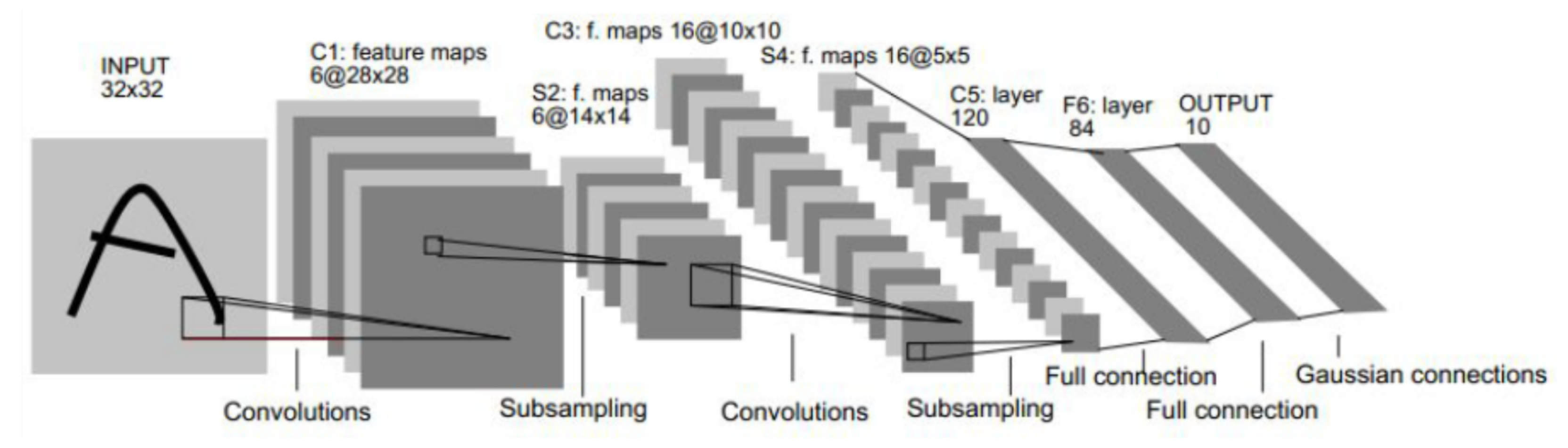
2.3. Convolutional Neural Network

The convolutional neural network (CNN), a widely used deep learning network, has played a significant role in computer vision (CV) [17,30,31]. In Figure 1, we illustrate a well-known CNN, LeNet-5, proposed by Yann Lecun [32] and composed of a convolution layer, pooling layer and a few layers of multilayer perceptron (MLP).

In the convolution layer, the input data such as images will be involved in the convolution by the convolution kernel and image features are extracted [18]. As shown in Formula (5), for the fth filter, $L_f^p\left(y\right)$ represents the pixel of the pth convolution layer at position y. For the cth channel, $L_c^{p-1}\left(x\right)$ represents the pixel of the preceding layer of the pth convolution layer at location x. m is the initial pixel for the ith element of filter $W_f^p$. $W_f^p\left(i\right)$ is the value of the fth filter of the pth convolution layer at location i, t is the total elements of filter $W_f^p$, and $b_f$ is the bias of the fth filter. The convolution kernel is the most important aspect in convolution calculation. There are some parameters in the kernel: one is the size of the kernel, e.g., $S\ast S\ast C\ast N$, where S is the size of the kernel, C is the depth of the kernel, and N is the number of kernels. The C is often determined by the depth of the input data—for example, an RGB image whose depth is three.

$$L_f^p\left(y\right)=\left(\sum _{c=1}^n\sum _{i=1,x=m}^{i=t,x=m+t}(W_f^p\left(i\right)\times L_c^{p-1}\left(x\right))\right)+b_f$$

(5)

The pooling layer is mainly used for data downsampling and image resolution reduction in the CNN [33]. The image data size will be greatly increased after one step of convolution, which can be reduced by using the pooling layer. Formula (6) shows the max pooling, which is one of the most common pooling methods, whose principle is to first select a region as the max pool’s size, and then look for the maximum value as the final value in this region. The next step involves sliding the max pool in the adjacent area and repeating the first stage of computing. Finally, all of the max or best values are combined to form a new matrix, which is the result of the pooling layer. As shown in Formula (6), M is the maximal layers in the yth location, $L\left(x\right)$ is the result of each convolution, and $pa{t}_h$,$pa{t}_w$ are the width and height of the convolution, respectively.

$$M_c^y\left(y\right)=max\left(L_f^s\left(x\right)\right)\mathrm{for}x=1,1\mathrm{to}pa{t}_h,pa{t}_w$$

(6)

The multilayer perceptron (MLP) layer’s function is to act as a classifier for the entire CNN model. The extracted feature map will be created after the input data have been subjected to a number of convolution and pooling layer operations. Then, the feature map is first transformed into one-dimensional data, which are processed to create a mapping relation from the feature data to the output data of N classes by MLP. MLP consists of multiple layers of a perceptron, and each layer operation is shown in Formula (7).

$$O_l=\sum _{k=1}^K\left(O_{l-1}\times W_{k,l}^{}\right)+b_l^{}$$

(7)

where $O_{l-1}$ represents the output of the last layer, W is the weight of the $k\mathrm{th}$ input feature in the $l\mathrm{th}$ layer, and $b_l$ represents the bias in the $l\mathrm{th}$ layer. $O_l$ represents the output of the $l\mathrm{th}$ layer, and K represents the total number of input features.

3. Methodology

Due to the complex operating conditions, the raw vibration signal of a rolling bearing is irregular and chaotic, and it is difficult to realize the effective feature extraction and accurate fault diagnosis by using the normal convolution neural network, especially when there is noise in the signals. Moreover, the over-fitting problem will occur due to noise and limited data. To address these problems, we introduce the two-domain learning of the raw signals to extract the key features adaptively by the composite dimension structure of the convolution neural network. Moreover, the dropout is added to solve the over-fitting.

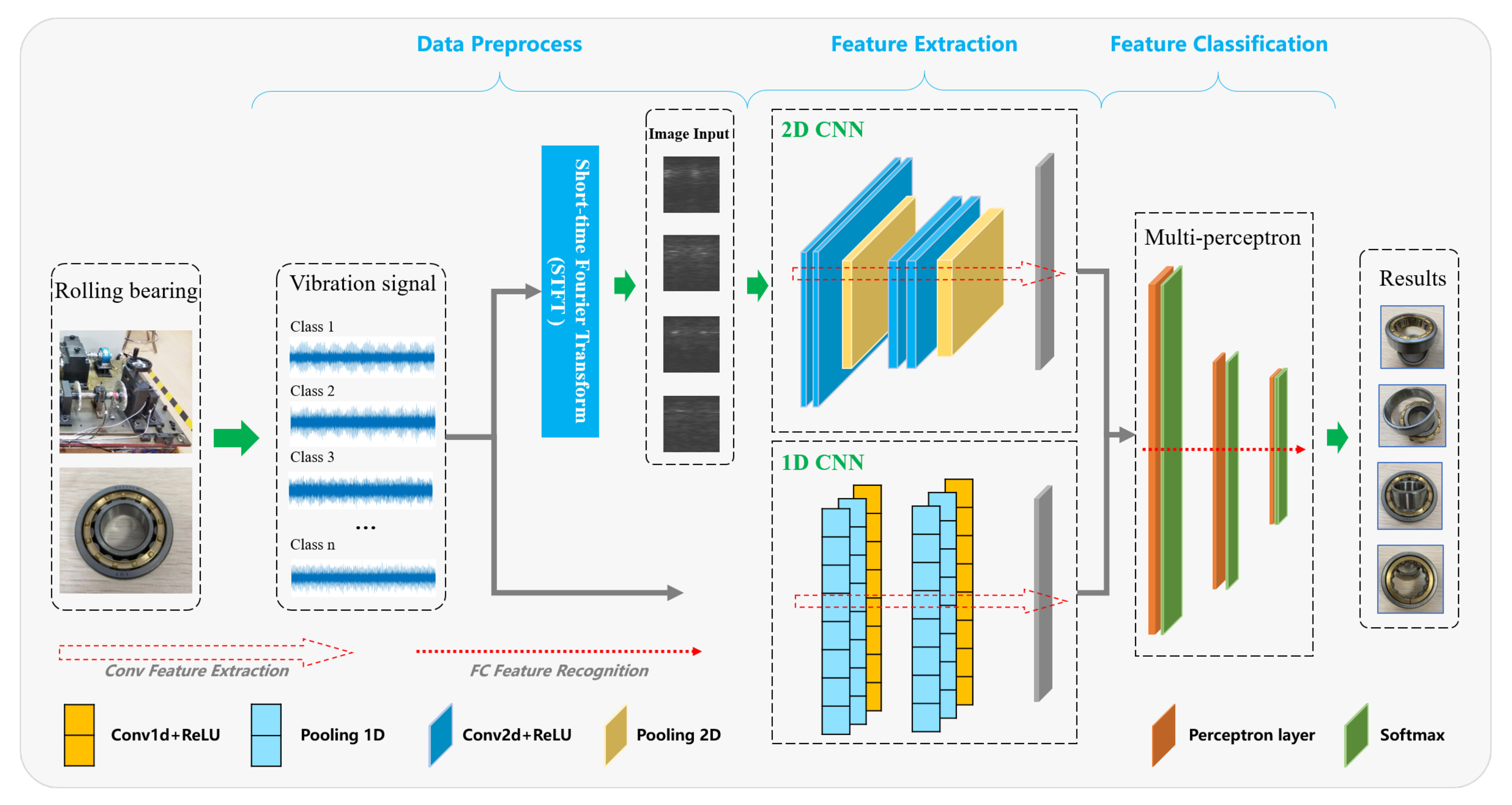
3.1. Proposed Model Structure

Considering the advantage of multi-domain learning, which can obtain more useful information from a raw sample, the first task is choosing another appropriate domain of data for the raw signal. Although the raw bearing vibration data are non-stationary series, the time–frequency domain contains more potential information of the bearing state according to the fault feature frequency of Formulas (1)–(3). Hence, the raw time series and time–frequency data are selected as the multi-domain supervised learning targets of our diagnostic model. On the other hand, the channel of the time-series and time–frequency data are of the one-dimensional and two-dimensional shape, respectively; the traditional two-dimensional (2D) convolution neural network cannot work on time-series data. As a result of the parallel structure of the neural network, the one-dimensional (1D) and two-dimensional (2D) convolution layers are used in our diagnostic model.

As mentioned above, the detailed fault diagnosis flow of our proposed method is shown in Figure 2, which contains three parts: the data preprocessing, feature extraction and feature classification. In the data preprocessing part, the first task is constructing the time–frequency domain data, and the raw vibration signal is transformed into a two-dimensional time–frequency image by the short-time Fourier transform (STFT). Not only does the STFT method retain the characteristic information of the vibration signal, but it also realizes the transformation from a 1D to a 2D signal. Then, the time–frequency image data and the raw time-series data are adopted as the diagnostic model input.

In the feature extraction part, parallel and different dimensional convolution layers are constructed, which are utilized to extract the key state feature information from the two shapes of data, respectively. The first group of 2D convolution layers are operating on the time–frequency image and extracting the useful features adaptively; the second 1D convolution layers are calculating the time-series and extracting the key information from the raw signal adaptively. Finally, two different and high-dimensional feature maps are acquired, which are merged and classified in the next step.

In the feature classification part, the main purpose is building the fault classification relationship form the extraction features to the bearing fault state. First, the two different shapes of feature maps of the previous convolution operation are fused into one by the average pooling operation. Then, the new feature map is inputted to the multiple fully connected layers, which form a mapping of feature data to fault state by a series of calculations on the neural nodes and hidden layers.

3.2. The Design of Hyper-Parameters

Our method also focuses on determining the structure of the neural network, such as the number of layers and neurons in convolutional layers, and the size of the convolution kernel, as well as the number of layers and neurons in the multilayer perceptron layer. The effect of model training will improve to some level when the number of network layers is increased, but the training time will continue to expand in logarithmic jumps at the same time. With some well-known network references [32,34] and a few samples for pre-testing, we chose an appropriate network architecture which combines two-layer 2D convolution, two-layer 1D convolution and a three-layer multilayer perceptron; a detailed description is shown in

Table 1. The proposed model structure.

Input	Layer 1	Layer 2	Layer 3	Layer 4	Layer 5	Output
1024	63 × 3	163 × 3	17,728	2048	512	10
129 × 129	65 × 5	165 × 5

.

Choosing one appropriate loss function will increase the model training velocity and achieve fast convergence. At present, there are a number of loss functions, such as minimum mean square error (MSE) and cross-entropy. This paper uses the cross-entropy loss as the loss value for the computation of the network. In comparison to MSE, the cross-entropy loss function can enhance the training effects of neural networks, particularly convolutional networks [35]. The cross-entropy loss function is shown in Formula (8).

$$L=\frac{1}{N}\sum _i{L}_i=\frac{1}{N}\sum _i-\sum _{c=1}^M{y}_{ic}\log \left(p_{ic}\right)$$

(8)

where M represents the number of total classes; $y_{ic}$ represents the variable 0 or 1 depending on whether the model output is the same as or different from the training sample label. $p_{ic}$ represents the predicted probability of the observed sample i belonging to category c.

The connection between the raw data and the output of the network model is a sophisticated non-linear mapping. Adding the activation function after each network layer can create a non-linear relation in the model. The most common activation functions are Sigmod, Tanh, ReLU, etc., as shown in Formulas (9)–(11). The ReLU activation function is selected through preliminary tests.

$$f\left(z\right)=\frac{1}{1+e^{-z}}$$

(9)

$$\tanh \left(x\right)=\frac{e^x-e^{-x}}{e^x+e^{-z}}$$

(10)

$$\mathrm{Relu}=\max (0,x)$$

(11)

Furthermore, the diagnostic model contains a number of parameters that need to be adjusted and optimized during the training process. However, the training data collected from the device constitute only a small proportion of the real situation, so are defect samples. Over-fitting will occur during the training process, i.e., using a model that yields good results in the training dataset, but poor effects on the test dataset or the newly collected data. To avoid this problem, our method employs the dropout technology. During model training, some hidden neurons’ nodes are dropped away at a certain probability, allowing the network to learn more complex features and enhance its generalization ability.

Meanwhile, the image data size will be modified after each convolution, as shown in Formula (12), and the size of the input data matrix shrinks. The data on the matrix’s edge have only been computed once, whilst the data at the matrix’s core have been computed numerous times, resulting in the edge data being lost. As a result, padding technology has been used, as shown in Formula (13), which means that the image’s outside circle is padded with 0 before each computation, preventing the original image from shrinking after numerous convolutions.

$$N=(W-F)/S+1$$

(12)

$$N=(W-F+2\ast P)/S+1$$

(13)

where W represents the size of image data, F represents the size of the convolution kernel, P represents the size of padding, S represents the step length of moving, and N represents the size of output data.

4. Experimental Validation

Two sets of bearing data will be used to test the proposed method and its effectiveness in diagnosing mechanical equipment: one from CWRU, which verifies the effect of the method on a vibration benchmark dataset, and the other from DUT’s machine vibration laboratory, which shows its generalization ability. Moreover, to prove the superiority of the method, various tests are performed with other methods to compare the proposed approach on the two datasets.

4.1. Case 1: CWRU Dataset Fault Diagnosis

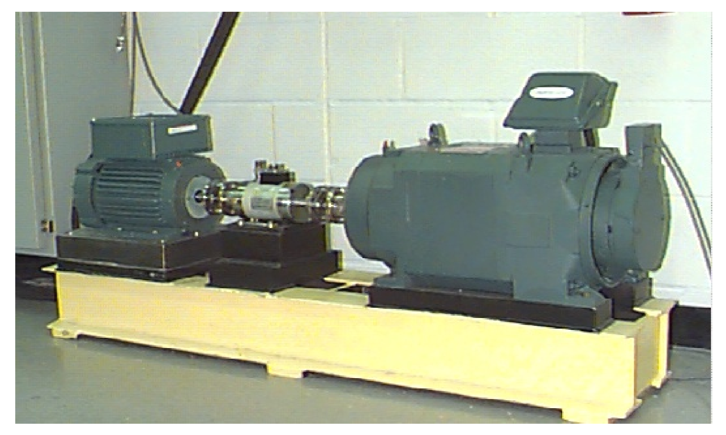
4.1.1. Data Introduction

One of the most commonly used standard datasets is the CWRU dataset [36]. Figure 3 shows the CWRU vibration test bench, which consists of a 2-horsepower motor, a torque sensor, a dynamo-meter and control electronics. The test bearing supports the motor shaft and is fitted with an SKF bearing. Each bearing unit’s fault is processed by electrical discharge machining (EDM). All bearing faults are divided into outer ring faults, inner ring faults and rolling ball faults. The flaw size is 0.007 to 0.021 inches. To properly design this experiment, a total of ten different types of defective bearing signals with various properties have been selected, with a sampling rate of 12 K.

Table 2. Specifications of CWRU dataset.

Index	Mark	Speed/RPM	Fault Degree	Fault Location
1	In7	1797	0.007${}^{″}$	Inner race
2	Ball7	1797	0.007${}^{″}$	Ball
3	Out7	1797	0.007${}^{″}$	Outer race
4	In14	1772	0.014${}^{″}$	Inner race
5	Ball14	1772	0.014${}^{″}$	Ball
6	Out14	1772	0.014${}^{″}$	Outer race
7	In21	1750	0.021${}^{″}$	Inner race
8	Ball21	1750	0.021${}^{″}$	Ball
9	Out21	1750	0.021${}^{″}$	Outer race
10	Norm	1797	-	Normal

gives the bearing dataset specifications, whereas

Table 3. Failure frequency of key components.

Inner Ring	Outer Ring	Cage Train	Rolling Element
5.4152	3.5848	0.39828	4.7135

contains the characteristic frequency of failure according to Formulas (1)–(3).

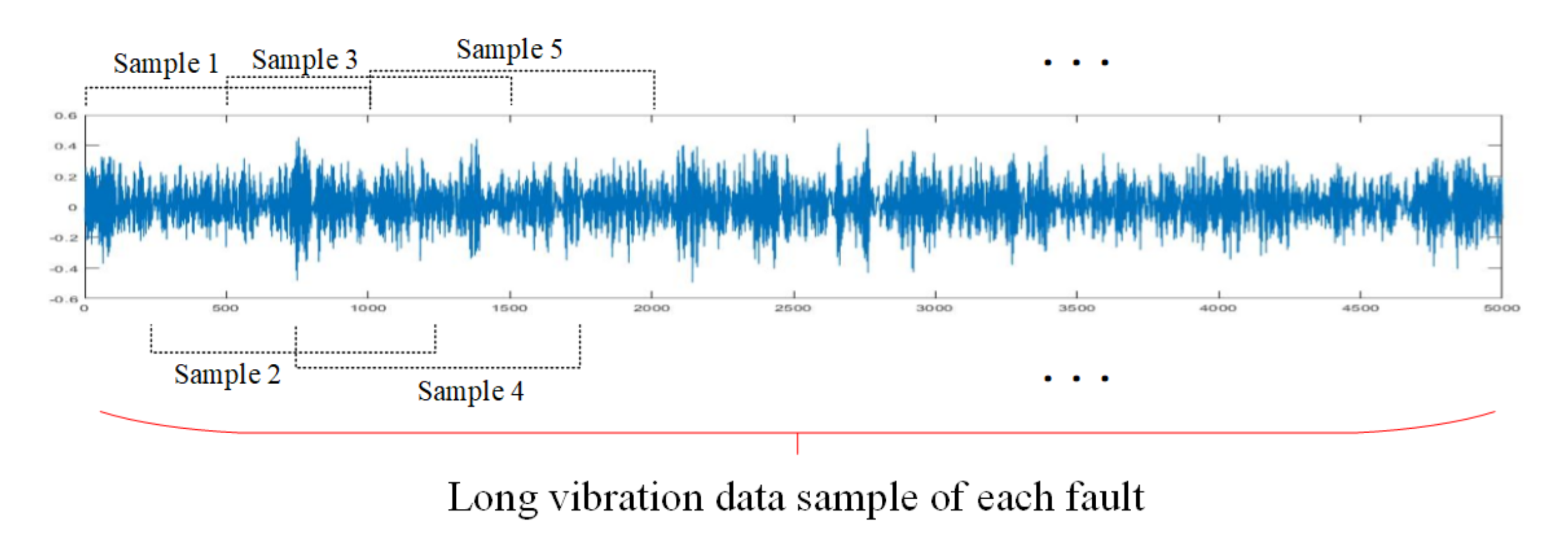
4.1.2. Data Pre-Processing

It can be seen that the vibration data of each type of fault are a long sequence of time-domain samples, which must be partitioned into several short samples as the original input of the diagnostic model. Meanwhile, the model’s training effects should be considered; both the total number of samples and the length of each individual sample will have an impact on the model’s training. The more samples there are, the more convergent and accurate the model training results. A short sample contains less feature information than a longer sample, but the length of sample and the numbers are inversely proportionate and irreconcilable. The sampling rate of the dataset is 12 K/s, the sampling period is 10 s, and each sample contains around 120,000 data points. Table 3 shows the fault characteristic frequency of three types of bearing unit (inner ring, outer ring and rolling elements). The bearing fault frequency is calculated by multiplying the characteristic frequency by the bearing roll speed of around 1800/rpm, which gives 162 Hz, 108 Hz and 141 Hz.

According to a bearing fault frequency of one and two, each short sample was selected from the raw data within 0.0853 s of the entire 10 s of data, resulting in 1024 points per sample. Moreover, the sample’s category label was formatted in one-hot style. As shown in Figure 4, the sample separation method with a 1024-point window and 256-point sliding length are utilized to split the raw sample. In total, there are 400 data samples for each type of fault and a total of 4000 data samples with 9 types of fault and one set of normal data in this bearing fault experiment. To better train and test the model, 400 data samples of each type of fault are split into two parts, 360 samples for training and 40 samples for testing, for a total of 3600 training samples and 400 testing samples.

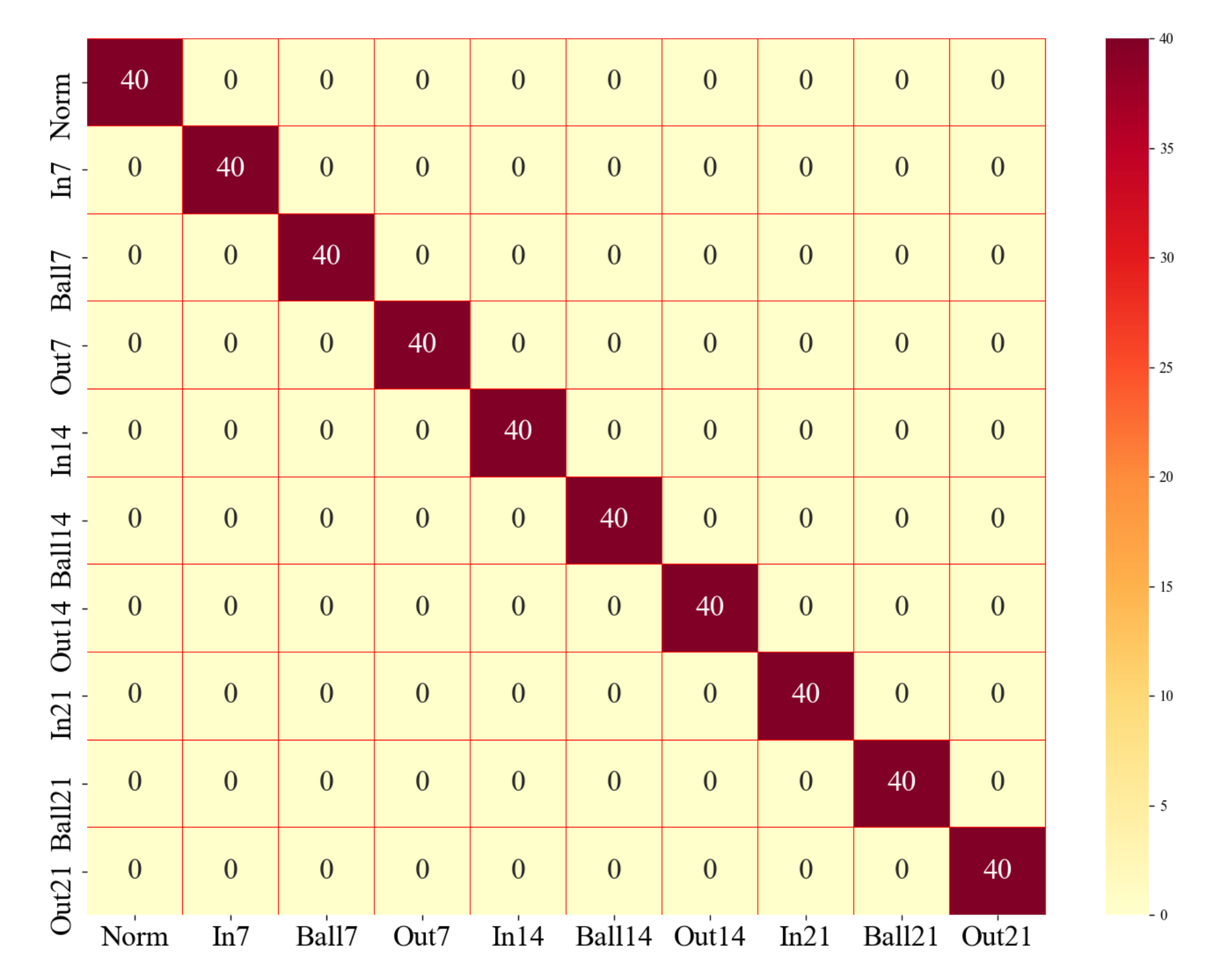
4.1.3. Model Training and Results

The platform configuration of diagnostic model training is shown as follows: the pytorch framework runs on a Windows 10 PC with an i9-10900k CPU, 64 GB of RAM and an RTX 3090 GPU. First, a single sample is transformed into a time–frequency image using the short-time Fourier transform (STFT). The window function of STFT is selected as ‘hann’ with a size of 256, and the overlapping points total 248. The obtained time–frequency image data are used as input to the 2D convolution layers. At the same time, the single raw samples are used to input to the 1D convolution layers.

In the full connection layers, the extracted feature maps that combine the output of 1D and 2D convolution layer operation are fed into the multilayer perceptron for training the fault feature classifier. The loss of cross-entropy is computed to correspond to the one-hot label of each sample. Finally, the diagnostic model is optimized by the Adam optimizer.

The results of this experiment, as well as the evaluation of the proposed method, are the loss value of model training and the classification accuracy of 400 testing samples. There are 50 training iterations, and the batch size and learning rate are 128 and 0.0001, respectively. The blue line in Figure 5 shows that the model loss value decreases as the number of training iterations increases. The loss value is below 0.001 after around 15 rounds, which shows that the model architecture is superior and the training process is effective. Forty samples of each state of bearing defect are used to test the model’s classification accuracy. A total of 400 data samples have been collected. The accuracy of the model varies as the number of iterations increases, as shown by the red line in Figure 5. After 15 iterations, the classification accuracy has reached nearly 100%, which indicates that the model training not only converges rapidly but also has high accuracy. Figure 6 shows the multi-class confusion matrix of the proposed method, and it can be seen that the 400 testing samples are all correctly predicted. Meanwhile, the model’s training process can be seen in Figure 5, in which variation trends are consistent.

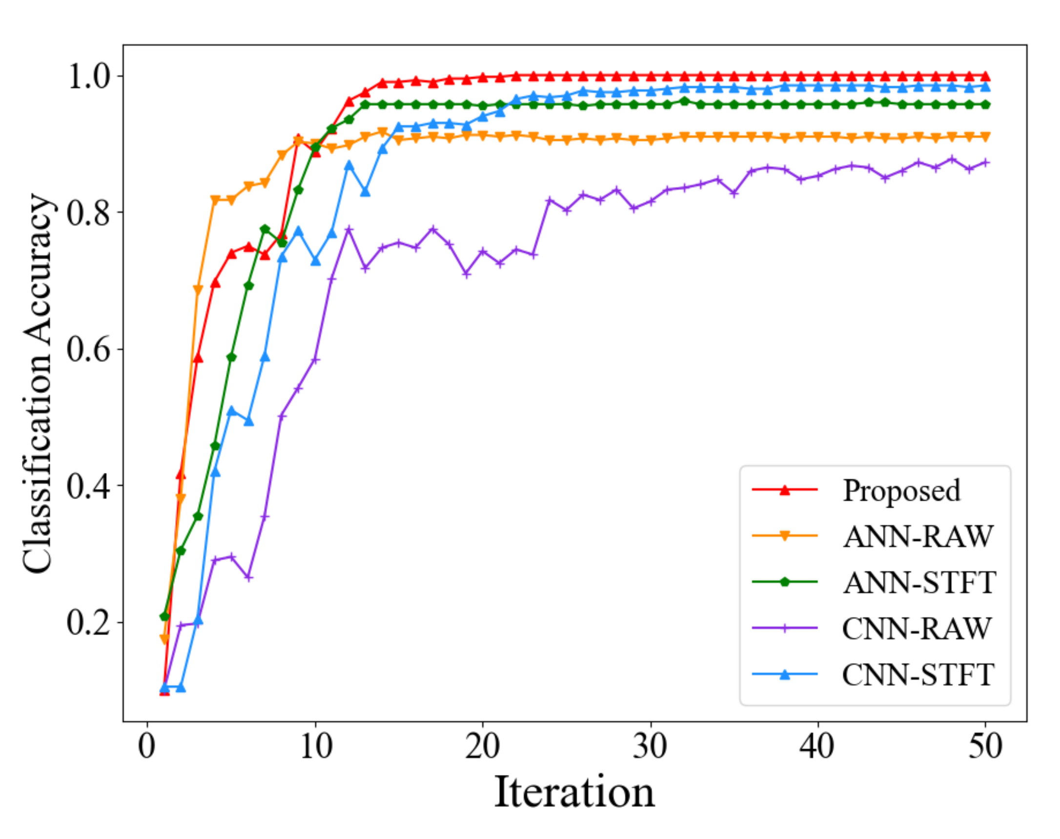
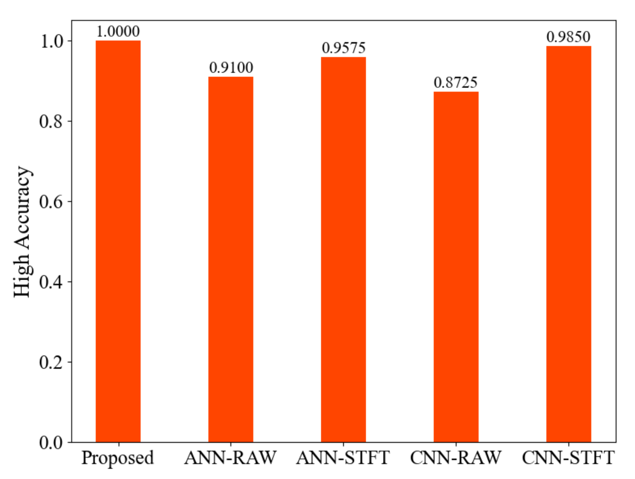
4.1.4. Comparative Analysis

To compare the superiority of the proposed method, four groups of experiments with four contrasting methods were designed. The first method (named ANN-RAW) is an artificial neural network (ANN) using the back propagation (BP) algorithm, in which the input data are the raw time-domain vibration signal. The second method (named ANN-STFT) is also the ANN, but the input data are the time–frequency image transformed from the vibration signal by the STFT. The third technique (named CNN-RAW) involves training and testing a normal convolutional network with raw time-series samples of vibration signals as input. Finally, the fourth technique (named CNN-STFT) was quoted from the document [37], which is the single-domain learning, and employs the same convolution network with the time–frequency data as input. All the models of the contrasting methods are trained by the 3600 samples and tested by the 400 samples, and each model’s training epoch is 50. Figure 7 and Figure 8 show the experimental results of these four techniques compared to the proposed method.

Figure 7 shows the fault prediction accuracy between the proposed and contrasting methods; all the methods’ classification accuracy rises rapidly during the first ten epoch times. The second ANN-STFT and fourth CNN-STFT methods rise faster than the other two contrasting methods, and reach accuracy of more than 90%. The last two methods, ANN-RAW and CNN-RAW, are only approximately 90%. However, comparing the accuracy of the four models, the proposed method has the highest accuracy of nearly 100%, as shown in Figure 8. In conclusion, the above experimental results on the CWRU dataset show that the suggested approach in this research is effective, and the classification accuracy of bearing defects is greater than previous approaches.

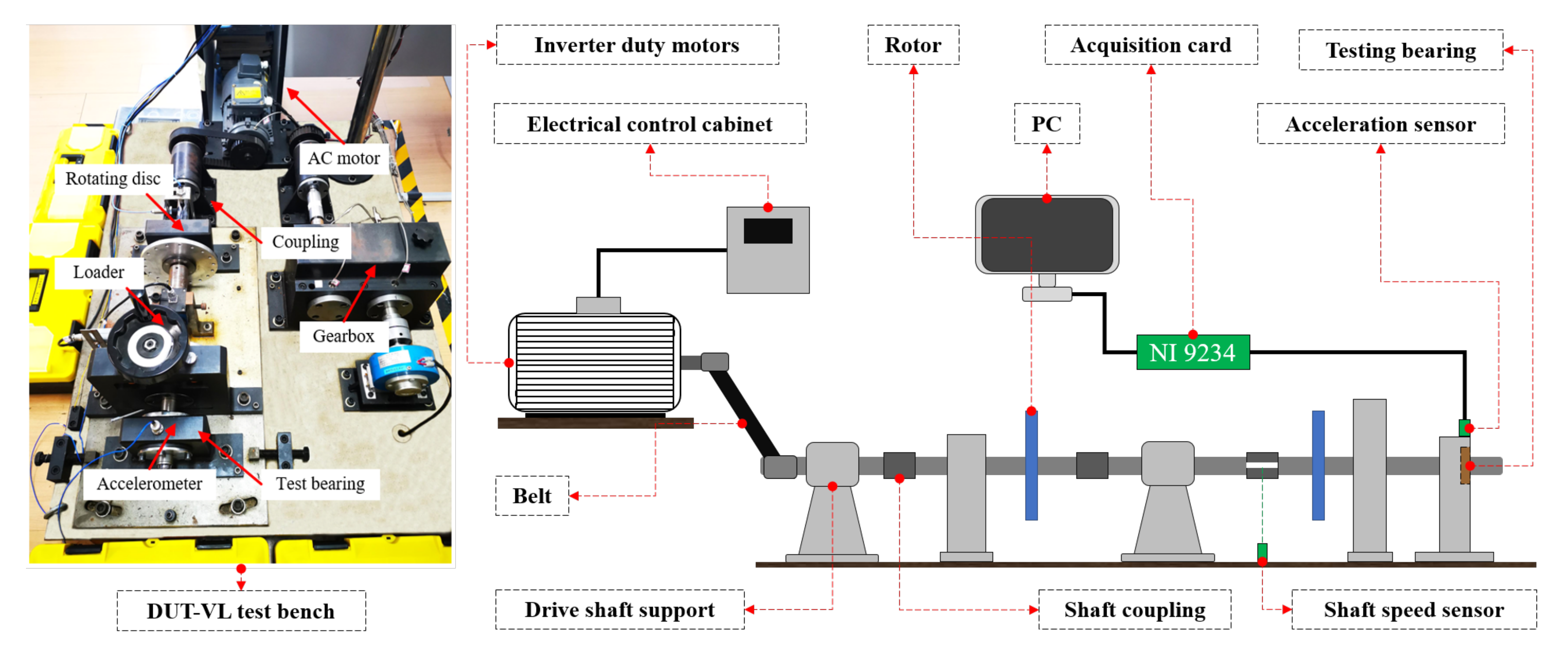
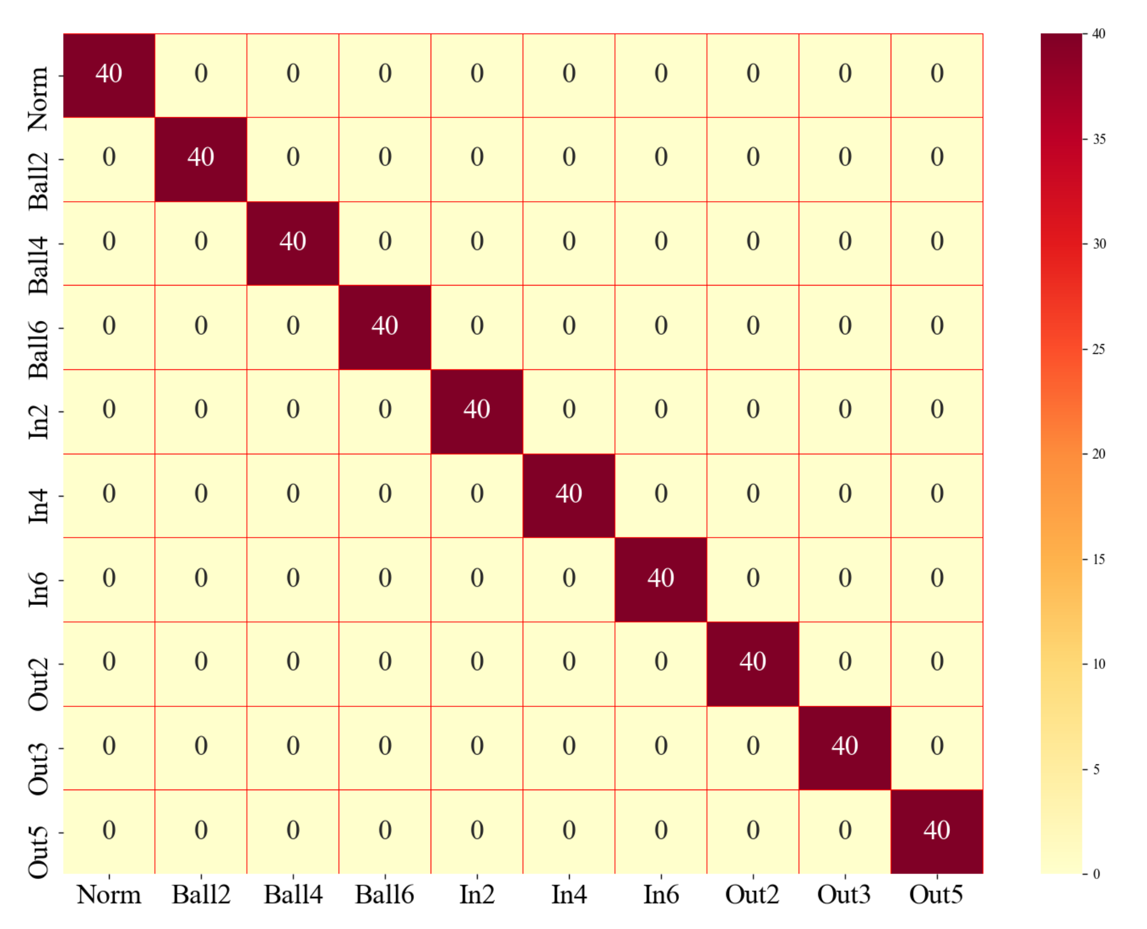
4.2. Case 2: DUT Lab Dataset Fault Diagnosis

4.2.1. Data Introduction

To further examine the efficacy and fault diagnostic ability of the proposed technique, we employed a test platform of rotating equipment at the DUT lab to simulate bearing failures and collect different failure state vibration data of rolling bearings. Figure 9 shows the bearing test platform, which is driven by a 220 V motor. A vibration acceleration sensor is installed in the vertical direction of the bearing pedestal. The bearing pedestal is equipped with an NU205EM detachable inner ring bearing or N205EM-A detachable outer ring bearing.

The NI 9234 with a four-channel acquisition card was chosen for vibration data collection, with the sampling frequency set to 10 kS/s and the sampling time set to 30 s. The bearing’s parameters are shown in

Table 4. Bearing specifications.

Type of Bearing	Inner Diameter	Outer Diameter	Width	Number of Ball
NU205	20	47	14	9
NU205EM	20	47	14	9

. A total of 9 varieties of abrasion faults, a type of normal bearing state, and a total of 10 bearing states were machined, aiming at different locations of rotational bearing faults and degrees of abrasion. Figure 10 and

Table 5. Specifications of DUT dataset.

Index	Mark	Fault Location	Fault Degree (mm)	Speed (rpm)
1	Norm	-	Normal	1200
2	Ball2	Ball	0.2	1200
3	Ball2	Ball	0.4	1200
4	Ball2	Ball	0.6	1200
5	In2	Inner race	0.2	1200
6	In2	Inner race	0.4	1200
7	In6	Inner race	0.6	1200
8	Out2	Outer race	0.2	1200
9	Out3	Outer race	0.36	1200
10	Out5	Outer race	0.54	1200

show the specific introduction and experimental settings for the ten types of bearing units.

4.2.2. Model Training and Results

The same data segmentation method as in Case 1 are utilized to split the long bearing state samples, but the sliding length is 512 points. The 1024 points of data are selected as a sample, and there are also 400 samples of each fault state, including 360 training samples and 40 test samples. In total, there are 3600 training samples and 400 test samples, which both contain 9 types of bearing unit faults and one normal bearing state.

In this test of the DUT dataset, the training model structure is the same as the one used in Case 1, and the model is trained with 3600 training samples. Using the same training rules as in the first experiment, this diagnostic model is trained for 50 iterations, and the classification accuracy of the model is tested by 400 samples. The blue line in Figure 11 shows the iterative loss value of the model training, and it can be observed that the loss of the model decreases quickly as the number of iterations increases. When the loss is less than 0.001, the loss decreases slowly and tends to a stable value, which shows that the model has a good convergence speed. In addition, the red line in Figure 11 depicts the model testing accuracy of 400 test samples. The accuracy grows dramatically as the number of iterations increases, and the accuracy rate approaches 100% in the first seven iterations. As shown in Figure 12, in the suggested method’s multi-class confusion matrix, all of the test samples are correctly labeled. The change in accuracy rate can also be considered consistent with the loss value change. That is, the faster the loss decreases, the faster the accuracy improves.

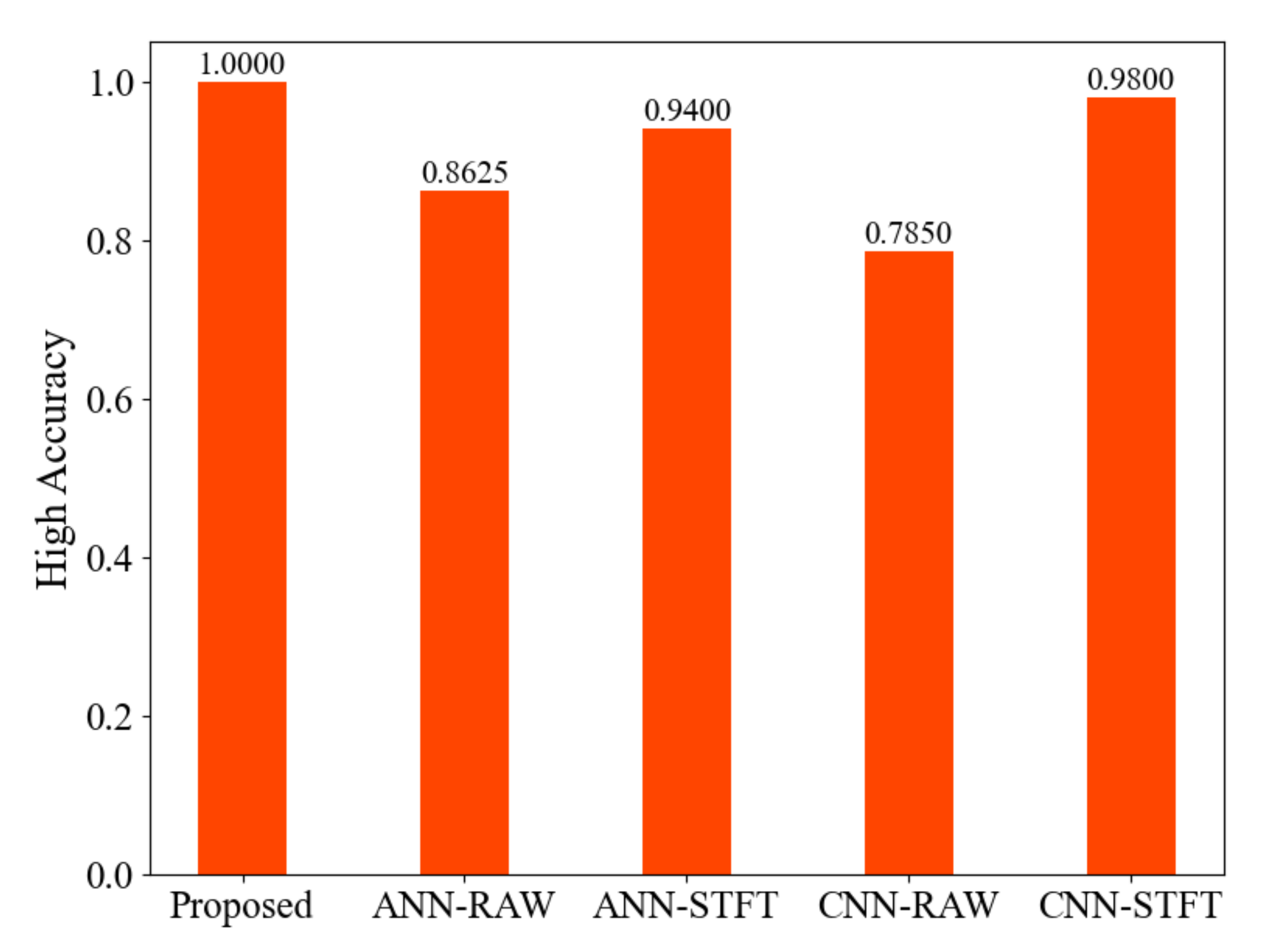
4.2.3. Comparative Analysis

Experiments with different sets of comparison techniques, similar to the Case 1 study, were designed to verify that the proposed method in the DUT dataset is the best. There were a total of five tests on the DUT dataset, which contained four comparison methods and our proposed method. The experimental results are shown in Figure 13 and Figure 14. Although the prediction accuracy of some methods, such as ANN-RAW, rose faster than the proposed method, the final prediction of the proposed approach was the highest at nearly 100%, as shown in Figure 13. From Figure 14, the accuracy of the other four techniques does not surpass 98%, remaining below the same contrasting method in Case 1. It is quite possible that the DUT dataset contains some noise, but the proposed method has also achieved highest prediction accuracy in the DUT dataset.

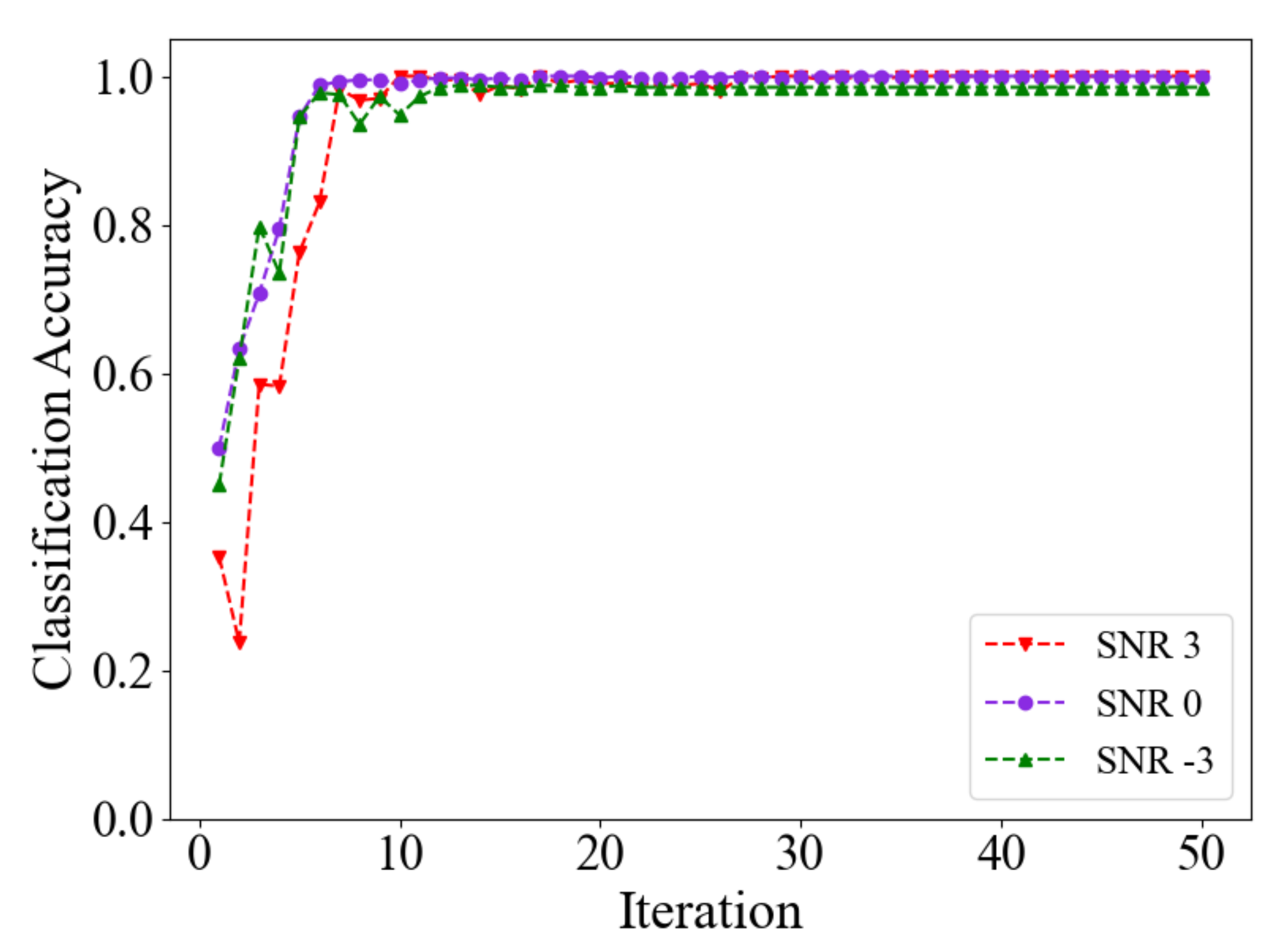
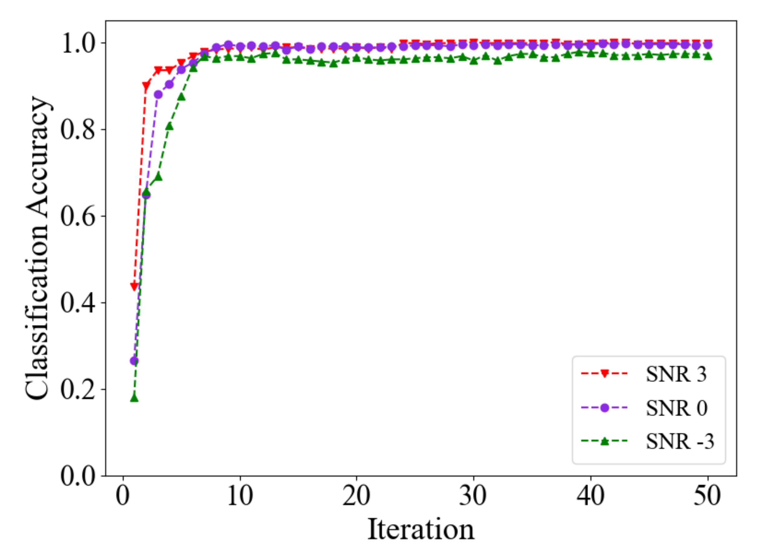
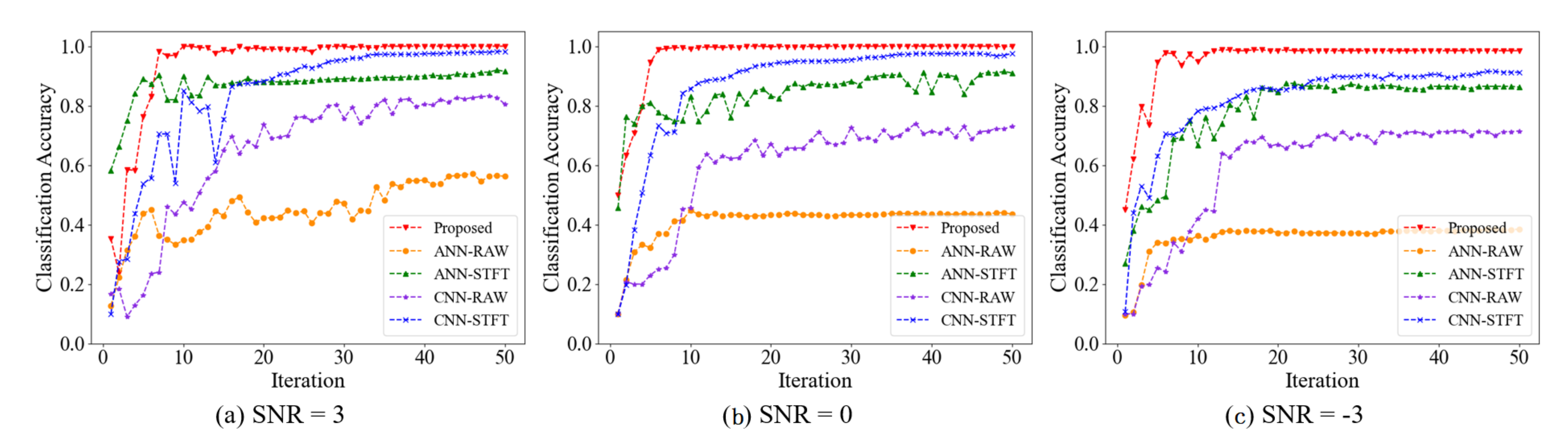
4.3. Noise: SNR3, SNR0, SNR-3

Due to the complex running environment in a real situation, the collected bearing vibration signals contain different degrees of noise signals, which will have an impact on the method of bearing fault diagnosis. Traditionally, denoising approaches are used to remove noisy signals; however, they can result in the loss of essential information or inadequate noise reduction, and manual experience is needed [38].

$$\mathrm{SNR}=\frac{P_{signal}}{P_{noise}}={\left(\frac{A_{signal}}{A_{noise}}\right)}^2$$

(14)

$$\mathrm{SNR}\left(\mathrm{dB}\right)=10{\log }_{10}\left(\frac{P_{signal}}{P_{noise}}\right)=20{\log }_{10}\left(\frac{A_{signal}}{A_{noise}}\right)$$

(15)

In Formulas (14) and (15), $P_{signal}$ denotes the power of the signal, $P_{noise}$ denotes the power of noise, $A_{signal}$ denotes the amplitude of the signal, and $A_{noise}$ denotes the amplitude of noise.

To demonstrate the robustness and generalization capabilities of the proposed approach in a strong noise environment, some noises are introduced to the raw signals of the CWRU and DUT datasets. Formulas (14) and (15) show the concept of the signal-to-noise ratio in the signal component. Then, we added Gaussian noise to the raw samples with SNRs of −3 db, 0 db and 3 db, equivalently adding 50%, 100% and 200% noise signals to the original signal’s energy. To begin with, these raw samples with varying SNRs were used to train the diagnostic model using the suggested approach, training 50 iterations.

Figure 15 shows the prediction accuracy on the CWRU dataset of the proposed method in different levels of noise. It reveals that when the SNR is 3 and 0, the models’ final prediction is at a high level of nearly 100 percent, indicating that the model trained with SNR 3 and 0 data performs well. It has no effect on the performance of fault classification when there is more than one instance of noise in the raw samples. Moreover, two instances of noise was added to the raw signal. As shown by the green line in Figure 15, the accuracy rate is reduced by several percentage points when compared to SNR 3 and SNR 0, indicating that the accuracy of the method proposed in this paper is affected slightly under strong noise, but it can still be maintained above 98.5 percent. Figure 16 depicts the same anti-noise performance of the proposed method on the DUT dataset; the prediction precision of the proposed method on noise of different SNRs is almost the same as the results on the CWRU dataset, and the accuracy is only a few percent lower than the latter.

At the same time, the raw data with three levels of SNR were tested by the four comparison methods. Figure 17 and Figure 18 show the different model training effects on the CWRU and DUT datasets with different signal-to-noise ratios, and there is a large difference in the classification accuracy of the bearing fault state.

From the first test on the CWRU dataset, the final prediction accuracies of all contrasting methods are significantly lower than the proposed method, and it becomes more obvious as the SNR decreases. When the SNR is −3, the highest accuracy of these methods, particularly the fourth method, CNN-STFT, is no more than 91.0%, which is far below the proposed method. The other methods’ efficiency is seriously affected by the noise components, and the first method, ANN-RAW, does not seem to operate. In addition, the different SNRs tested on the DUT dataset also yield the same performance compared to the CWRU dataset, as shown in Figure 18. The identification precision of the contrasting methods also decreases rapidly with the increasing noise components, and it is less than 90% when the SNR is −3. These experimental results demonstrate the superiority of the introduced method under a strong noise environment.

4.4. Comparison with Other Research and Efficiency Evaluation of Algorithm

There are also some studies about bearing fault diagnosis with different methods. Piltan [39] proposed an algorithm of an intelligent digital twin integrated with machine learning for bearing anomaly detection and crack size identification. Although this method achieves a good result for fault state classification with a more than 98.7% accuracy rate, this paper uses a machine learning method combined with the intelligent digital twin model, and expert knowledge is needed to build the model. Our method achieves good bearing fault state classification with the same accuracy of more than 99.9%, but no manual experience is needed, and it is an end-to-end diagnostic method. In Tagawa’s research [22], a new algorithm is proposed for anomaly detection from noisy data, which contains a series of complicated signal analyses for denoising and the extraction of useful information. However, using parallel convolution layers, our method can extract critical fault features adaptively from signals disrupted by high noise and achieve high fault state prediction accuracy.

Although our method achieves a good result for rolling bearing fault state classification on the two datasets, it is necessary to consider the computational performance and the efficiency of the proposed algorithm. Hence, the efficiency of our improved algorithm was measured by the calculation time of Case 1, which contained two parts: the time for model training and the time for model diagnosis. In the first part, our method aims to train a diagnostic model from the training data. As the model training process includes many iterative epochs, it is time-consuming, with 383.780 s, which is shown in

Table 6. The efficiency of proposed and contrasting algorithms.

Operation Time	Proposed Method	ANN-RAW	ANN-STFT	CNN-RAW	CNN-STFT
Training time/s	383.78	29.137	363.298	39.153	361.604
Diagnosis time/s	0.758	0.129	0.703	0.142	0.642

. Comparing the other methods, the operation time of the proposed technology is the longest, as it includes two-domain data learning. It should be pointed out that once the diagnostic model has been trained, the training process is not ongoing and the trained model can operate for bearing state diagnosis. As shown in Table 6, it can be seen that the diagnosis time of the proposed method does not exceed 1 s and is close to other methods, i.e., the trained model can identify the accurate bearing state from the raw signal within 1 s. In conclusion, our proposed algorithm performs well in fault diagnosis, in terms of both the prediction accuracy and the algorithm efficiency.

4.5. Discussion

(1)

In this section, the effectiveness of the proposed approach was verified on two datasets: the CWRU and DUT datasets. The proposed fault diagnosis model performs well both in the training and testing steps. The prediction accuracy of fault states is more than 99.9% and is superior to the contrasting methods. Due the advantage of multi-domain learning, our proposed method extracts the fault features adaptively and realizes state prediction from the raw rolling bearing data in an end-to-end manner. Compared to the traditional fault diagnosis methods, there is no complicated feature extraction and no prior knowledge required.

(2)

To simulate the complicated operation conditions, different SNR noise was added to the raw samples for testing the anti-noise ability of the proposed method. The results show that the raw signal was disturbed by strong noise, but our method still achieves high classification accuracy of the fault state. The prediction accuracy of the proposed approach is slightly lower than in the test on raw data but higher than the contrasting methods, and this demonstrates the generalization ability and robustness of our methods. Moreover, the experimental results of calculation time show that our proposed algorithm is simple and effective and achieves high prediction within a short time.

5. Conclusions and Prospects

Due to the non-stationarity and non-linearity of raw rolling bearing vibration signals, it is difficult to handle feature extraction and state classification adaptively, especially in a complicated environment. This paper proposes a bearing failure diagnostic approach that employs two-domain supervised learning of a CNN, and the diagnostic model realizes the fault state prediction by the fusion of two-domain information. The main contributions of this paper can be described as follows:

(1)

It constructs a new fault diagnosis model that combines the one-dimensional and two-dimensional convolution layers for learning multi-domain information of bearing faults; this model fully extracted the bearing fault features from time–frequency and raw time-domain data of bearing vibration signals.

(2)

The constructed multilayer perceptron establishes the mapping between feature matrix and fault state. The dropout technology is introduced to prevent the model over-fitting, and the diagnostic model performs well both in training and testing.

(3)

To validate the effectiveness of the proposed method, two experiments are performed on the CWRU and DUT datasets. Some different SNR noise is also added to the raw signals, and the results prove that the method proposed is effective. It also shows a generalization ability that can identify the fault state from the raw signal accurately in the strong noise condition.

Although this proposed method achieves good results, the vibration signals are all collected at a constant speed and steady state. It is not considered that the vibration dataset is under variable conditions. Next, we will focus on bearing fault diagnosis under variable conditions.

References

1. Lu, Y.; Ding, E.J.; Du, J.; Chen, G.C.; Zheng, Y. Safety detection approach in industrial equipment based on RSSD with adaptive parameter optimization algorithm. Saf. Sci. 2020, 125, 104605. [Google Scholar] [CrossRef]
2. Shen, C.; Qi, Y.; Wang, J.; Cai, G.; Zhu, Z. An automatic and robust features learning method for rotating machinery fault diagnosis based on contractive autoencoder. Eng. Appl. Artif. Intell. 2018, 76, 170–184. [Google Scholar] [CrossRef]
3. Hui, K.H.; Lim, M.H.; Leong, M.S.; Al-Obaidi, S.M. Dempster-Shafer evidence theory for multi-bearing faults diagnosis. Eng. Appl. Artif. Intell. 2017, 57, 160–170. [Google Scholar] [CrossRef]
4. Zhang, Z.; Chen, H.; Li, S.; An, Z. Unsupervised domain adaptation via enhanced transfer joint matching for bearing fault diagnosis. Measurement 2020, 165, 108071. [Google Scholar] [CrossRef]
5. Xu, X.L.; Yu, Z.W. Failure analysis of tapered roller bearing inner rings used in heavy truck. Eng. Fail. Anal. 2020, 111, 104474. [Google Scholar] [CrossRef]
6. Chegini, S.N.; Bagheri, A.; Najafi, F. Application of a new EWT-based denoising technique in bearing fault diagnosis. Measurement 2019, 144, 275–297. [Google Scholar] [CrossRef]
7. Zhang, X.; Liu, Z.; Wang, L.; Zhang, J.; Han, W. Bearing fault diagnosis based on sparse representations using an improved OMP with adaptive Gabor sub-dictionaries. ISA Trans. 2020, 106, 355–366. [Google Scholar] [CrossRef]
8. Kim, Y.; Park, J.; Na, K.; Yuan, H.; Youn, B.D.; Kang, C.S. Phase-based time domain averaging (PTDA) for fault detection of a gearbox in an industrial robot using vibration signals. Mech. Syst. Signal Process. 2020, 138, 106544. [Google Scholar] [CrossRef]
9. Li, H.; Liu, T.; Wu, X.; Chen, Q. An optimized VMD method and its applications in bearing fault diagnosis. Measurement 2020, 166, 108185. [Google Scholar] [CrossRef]
10. Ma, J.; Wu, J.; Wang, X. Incipient fault feature extraction of rolling bearings based on the MVMD and Teager energy operator. ISA Trans. 2018, 80, 297–311. [Google Scholar] [CrossRef]
11. He, C.; Niu, P.; Yang, R.; Wang, C.; Li, Z.; Li, H. Incipient rolling element bearing weak fault feature extraction based on adaptive second-order stochastic resonance incorporated by mode decomposition. Measurement 2019, 145, 687–701. [Google Scholar] [CrossRef]
12. Shao, K.; Fu, W.; Tan, J.; Wang, K. Coordinated approach fusing time-shift multiscale dispersion entropy and vibrational Harris hawks optimization-based SVM for fault diagnosis of rolling bearing. Measurement 2021, 173, 108580. [Google Scholar] [CrossRef]
13. Zhang, X.; Zhang, Q.; Chen, M.; Sun, Y.; Qin, X.; Li, H. A two-stage feature selection and intelligent fault diagnosis method for rotating machinery using hybrid filter and wrapper method. Neurocomputing 2018, 275, 2426–2439. [Google Scholar] [CrossRef]
14. Jiang, F.; Zhu, Z.; Li, W.; Ren, Y.; Zhou, G.; Chang, Y. A fusion feature extraction method using EEMD and correlation coefficient analysis for bearing fault diagnosis. Appl. Sci. 2018, 8, 1621. [Google Scholar] [CrossRef] [Green Version]
15. Guo, G.; Zhang, N. A survey on deep learning based face recognition. Comput. Vis. Image Underst. 2019, 189, 102805. [Google Scholar] [CrossRef]
16. Lei, Y.; Yang, B.; Jiang, X.; Jia, F.; Li, N.; Nandi, A.K. Applications of machine learning to machine fault diagnosis: A review and roadmap. Mech. Syst. Signal Process. 2020, 138, 106587. [Google Scholar] [CrossRef]
17. Yu, H.; Yang, L.T.; Zhang, Q.; Armstrong, D.; Deen, M.J. Convolutional neural networks for medical image analysis: State-of-the-art, comparisons, improvement and perspectives. Neurocomputing 2021, 444, 92–110. [Google Scholar] [CrossRef]
18. Banik, P.P.; Saha, R.; Kim, K.D. An automatic nucleus segmentation and CNN model based classification method of white blood cell. Expert Syst. Appl. 2020, 149, 113211. [Google Scholar] [CrossRef]
19. Ban, J.E.; Rho, B.H.; Kim, K.W. A study on the sound of roller bearings operating under radial load. Tribol. Int. 2007, 40, 21–28. [Google Scholar] [CrossRef]
20. Liu, Z.; Tang, X.; Wang, X.; Mugica, J.E.; Zhang, L. Wind turbine blade bearing fault diagnosis under fluctuating speed operations via Bayesian augmented Lagrangian analysis. IEEE Trans. Ind. Inform. 2020, 17, 4613–4623. [Google Scholar] [CrossRef]
21. Chen, J.; Pan, J.; Li, Z.; Zi, Y.; Chen, X. Generator bearing fault diagnosis for wind turbine via empirical wavelet transform using measured vibration signals. Renew. Energy 2016, 89, 80–92. [Google Scholar] [CrossRef]
22. Tagawa, Y.; Maskeliūnas, R.; Damaševičius, R. Acoustic Anomaly Detection of Mechanical Failures in Noisy Real-Life Factory Environments. Electronics 2021, 10, 2329. [Google Scholar] [CrossRef]
23. Abdelkader, R.; Kaddour, A.; Derouiche, Z. Enhancement of rolling bearing fault diagnosis based on improvement of empirical mode decomposition denoising method. Int. J. Adv. Manuf. Technol. 2018, 97, 3099–3117. [Google Scholar] [CrossRef]
24. Guo, X.; Shen, C.; Chen, L. Deep fault recognizer: An integrated model to denoise and extract features for fault diagnosis in rotating machinery. Appl. Sci. 2016, 7, 41. [Google Scholar] [CrossRef]
25. Yan, X.; Jia, M. A novel optimized SVM classification algorithm with multi-domain feature and its application to fault diagnosis of rolling bearing. Neurocomputing 2018, 313, 47–64. [Google Scholar] [CrossRef]
26. Mohanty, S.; Gupta, K.K.; Raju, K.S. Hurst based vibro-acoustic feature extraction of bearing using EMD and VMD. Measurement 2018, 117, 200–220. [Google Scholar] [CrossRef]
27. Manhertz, G.; Bereczky, A. STFT spectrogram based hybrid evaluation method for rotating machine transient vibration analysis. Mech. Syst. Signal Process. 2021, 154, 107583. [Google Scholar] [CrossRef]
28. Marquezino, F.L.; Portugal, R.; Sasse, F. Obtaining the Quantum Fourier Transform from the classical FFT with QR decomposition. J. Comput. Appl. Math. 2010, 235, 74–81. [Google Scholar] [CrossRef] [Green Version]
29. Li, L.; Cai, H.; Han, H.; Jiang, Q.; Ji, H. Adaptive short-time Fourier transform and synchrosqueezing transform for non-stationary signal separation. Signal Process. 2020, 166, 107231. [Google Scholar] [CrossRef]
30. Fujiyoshi, H.; Hirakawa, T.; Yamashita, T. Deep learning-based image recognition for autonomous driving. IATSS Res. 2019, 43, 244–252. [Google Scholar] [CrossRef]
31. Tian, C.; Fei, L.; Zheng, W.; Xu, Y.; Zuo, W.; Lin, C.W. Deep learning on image denoising: An overview. Neural Netw. 2020, 131, 251–275. [Google Scholar] [CrossRef] [PubMed]
32. LeCun, Y.; Bottou, L.; Bengio, Y.; Haffner, P. Gradient-based learning applied to document recognition. Proc. IEEE 1998, 86, 2278–2324. [Google Scholar] [CrossRef] [Green Version]
33. Singh, P.; Raj, P.; Namboodiri, V.P. EDS pooling layer. Image Vis. Comput. 2020, 98, 103923. [Google Scholar] [CrossRef]
34. Li, C.; Li, S.; Zhang, A.; He, Q.; Liao, Z.; Hu, J. Meta-learning for few-shot bearing fault diagnosis under complex working conditions. Neurocomputing 2021, 439, 197–211. [Google Scholar] [CrossRef]
35. Bosman, A.S.; Engelbrecht, A.; Helbig, M. Visualising basins of attraction for the cross-entropy and the squared error neural network loss functions. Neurocomputing 2020, 400, 113–136. [Google Scholar] [CrossRef] [Green Version]
36. Loparo, K.A. Case Western Reserve University Bearing Data Center. In Bearings Vibration Data Sets; Case Western Reserve University: Cleveland, OH, USA, 2012. [Google Scholar]
37. Pandhare, V.; Singh, J.; Lee, J. Convolutional neural network based rolling-element bearing fault diagnosis for naturally occurring and progressing defects using time-frequency domain features. In Proceedings of the 2019 Prognostics and System Health Management Conference (PHM-Paris), Paris, France, 2–5 May 2019; pp. 320–326. [Google Scholar]
38. Beale, C.; Niezrecki, C.; Inalpolat, M. An adaptive wavelet packet denoising algorithm for enhanced active acoustic damage detection from wind turbine blades. Mech. Syst. Signal Process. 2020, 142, 106754. [Google Scholar] [CrossRef]
39. Piltan, F.; Kim, J.M. Bearing anomaly recognition using an intelligent digital twin integrated with machine learning. Appl. Sci. 2021, 11, 4602. [Google Scholar] [CrossRef]
Figure 1. LeNet-5.
Energies 15 04614 g001
Figure 2. The proposed method of this paper.
Energies 15 04614 g002
Figure 3. Case Western Reserve University bearing test bed.
Energies 15 04614 g003
Figure 4. Schematic diagram of sample collection.
Energies 15 04614 g004
Figure 5. The loss and classification accuracy of proposed method on CWRU dataset.
Energies 15 04614 g005
Figure 6. Multi-class confusion matrix of proposed method on CWRU dataset.
Energies 15 04614 g006
Figure 7. The classification accuracy between proposed and compared methods on CWRU dataset.
Energies 15 04614 g007
Figure 8. The highest classification accuracy between proposed and compared methods on CWRU dataset.
Energies 15 04614 g008
Figure 9. Dalian University of Technology bearing test platform.
Energies 15 04614 g009
Figure 10. Fault types of bearings.
Energies 15 04614 g010
Figure 11. The results of model training on DUT dataset.
Energies 15 04614 g011
Figure 12. Multi-class confusion matrix of proposed method on DUT dataset.
Energies 15 04614 g012
Figure 13. The classification accuracy between proposed and compared methods on DUT dataset.
Energies 15 04614 g013
Figure 14. The highest classification accuracy between proposed and compared methods on DUT dataset.
Energies 15 04614 g014
Figure 15. The results of model training on different noise levels (testing on CWRU dataset).
Energies 15 04614 g015
Figure 16. The results of model training on different noise levels (testing on DUT dataset).
Energies 15 04614 g016
Figure 17. The classification accuracy of different methods under different SNRs (testing on CWRU dstaset).
Energies 15 04614 g017
Figure 18. The classification accuracy of different methods under different SNRs (testing on DUT dstaset).
Energies 15 04614 g018