A Simplified Solution Method for End-of-Term Storage Energy Maximization Model of Cascaded Reservoirs

Abstract

In medium-term scheduling, the end-of-term storage energy maximization model is proposed to create conditions for the safety, stability and economic operation of the hydropower system after control term, which satisfies the system load demand undertaken by the cascaded system in a given scheduling period. This paper presents a simplified solution method based on the Lagrangian relaxation method (LR) to solve the end-of-term storage energy maximization model. The original Lagrange dual problem with multiple Lagrange multipliers is converted to that with only one Lagrange multiplier by an entropy-based aggregate function method, which relaxes the complex cascaded hydropower system load balance constraints. The subgradient method and successive approximation of dynamic programming (DPSA) are adopted to update the Lagrange multiplier iteratively and solve the subproblem of the Lagrange dual problem, respectively. The Wujiang cascaded hydropower system is studied, and the result shows that the simplified solution method for the end-of-term storage energy maximization model both improves solving efficiency and ensures solving accuracy to a great extent.

1. Introduction

Hydropower energy has the characteristics of low pollution, easy maintenance and high flexibility [1]. A reservoir and the power grid are linked by each hydropower station in a cascaded hydropower system, which utilize compensation coordination among the reservoirs with regard to the overall benefit [2]. Through the economic operation of the hydropower system, the compensation coordination between reservoirs can be effectively utilized to improve the utilization of hydropower resources, and the flexibility of hydropower can be fully utilized to meet the different needs of the hydropower system through the regulation of the hydropower system. In general, the economic operation of the hydropower system is divided into conventional dispatching and optimal dispatching. It can meet the different needs of the power system by establishing optimal dispatching models with different objectives, which can be divided into two modes: regulating power generation by water supply and regulating impoundment by power generation. The objective function of regulating power generation by water supply contains power generation maximization, power generation benefit maximization, minimum output maximization [3] and peak regulating power maximization [4]. In contrast, the objective function of regulating impoundment by power generation contains maximum end-of-term storage energy and minimum energy consumption. In order to solve these optimal operation models, more and more optimization techniques and heuristic algorithms [5,6] have been applied in the past few decades, such as linear programming (LP) [7], nonlinear programming (NLP) [8], dynamic programming (DP) [9,10,11], genetic algorithm (GA) [12], particle swarm optimization (PSO) [13] and ant colony algorithm (ACO) [14]. DPSA [15,16] and progressive optimality algorithm (POA) are both approximate dynamic programming methods, which deal with the curse of dimension. Trott and Yeh developed DPSA, which decomposes the original problem into a series of subproblems, whose optimization sequence converges back to the original one to maximize net benefits [16]. Giles and Wunderlich adopted DPSA to solve the minimum total operation cost model, which determines end-of-week levels for 52 weeks or shorter planning periods for 19 storage reservoirs [15]. Opan applied DPSA to solve optimization and simulation models for a water resource system with multiple reservoirs in the Ceyhan Basin of Turkey [17]. Zhang et al. presented a hybrid algorithm, which uses DPSA to reduce the spatial dimensionality and adopts an improved POA to alleviate the temporal dimensionality to minimize the flood peak optimal model for multiple reservoirs [18]. He et al. proposed an improved DPSA with a relaxation strategy based on the approximate concavity and monotonicity characteristics of the power generation utility function of DPSA to solve the long-term joint power generation scheduling [19]. Even so, the optimal operation models with complicated side constraints are limited by strong constraints and solved with difficulty.

In recent decades, LR [20,21] has been widely applied to solve hydropower scheduling problem, such as hydropower system load allocation and hydro unit commitment [22,23,24,25], which contains complicated side constraints. LR converts the optimal operation model to a dual problem, which contains constraints with a high degree of structure [26]. In addition, the optimal operation model is solved by a set of disjoint subproblems and the Lagrange multiplier iteration. Pursimo et al. presented an optimal feedback control method using a quadratic cost function for the hydro scheduling problem, which took constraints into account by the Lagrange multipliers [27]. Redondo and Cenejo studied the Lagrange multipliers iterative update method solving the dual problem of the short-term hydrothermal coordination problem, such as the subgradient method, cutting plane method (CP), bundle method (BD) and dynamically constrained cutting plane method (DC-CP) [23]. Guan et al. presented an optimization-based algorithm using LR to solve hydro subproblems with cascaded reservoirs and discrete hydro constraints, which uses a set of multipliers to substitute out the reservoir dynamic and to relax the reserve level constraints [22]. Soares et al. presented a heuristic procedure based on LR to solve the dynamic dispatch problem of scheduling generation in which a problem is decomposed into two subproblems: a unit commitment subproblem (UC) and a generation dispatch subproblem (GD) [24]. Wang relaxed the constraints on the plant-based operating region and systemwide spinning reserve of a Fujian hydro system introducing the Lagrange multipliers so that the primal optimization problem is decomposed into a hydro subproblem solved with the improved simplex-like method and individual hydro plant subproblems solved by dynamic programming [28]. Finardi, Takigawa and Brito verified that LR is the approach with the best overall performance as the problem increases in that it is less sensitive to variations in the input data or the problem, which leads to a low processing time and a good quality solution [29]. Liu et al. converted the chance constraint for controlling the system failures on power generation to a dual problem through LR [30]. However, the relationship among multiple Lagrange multipliers results in a much longer solving time for a large-scale hydropower system optimal operation model.

The end-of-term storage energy maximization model for medium-term scheduling of cascaded reservoirs is a high-dimensional, nonlinear and large-scale optimization problem, which contains complex cascaded hydropower system load balance constraints. The complex cascaded system load balance constraint can be relaxed into the objective function by LR, and the optimal solution can be obtained by solving the Lagrange duality problem and iterating the Lagrange multiplier. However, in previous studies, the end-of-term storage energy maximization model was decomposed into a generation scheduling subproblem for each period by LR, requiring an iterative solution of the multiple Lagrange multipliers. Therefore, this paper proposes a simplified solution method for end-of-term storage energy maximization model for medium-term scheduling, which transforms the cascaded hydropower system load balance constraints into a Lagrange dual problem with only one Lagrange multiplier by means of an entropy-based aggregate function method. The subproblem is solved by DPSA, and the Lagrange multiplier is updated iteratively by the subgradient method. Then, the Wujiang cascaded hydropower system is studied. It can be concluded that the simplified solution method of an end-of-term storage energy maximization model greatly improves the solution efficiency and ensures the solution accuracy.

2. Materials and Methods

The medium-term dispatching of a hydropower system refers to the optimal dispatching, which takes 1 day as the dispatching stage length and the next few days as the dispatching term. The medium-term dispatching of a hydropower system includes two dispatching modes: “regulating power generation by water supply” and “regulating impoundment by power generation”. The mode, called “regulating impoundment by power generation”, refers to the load distribution of the given total output process of a cascaded or multiple cascaded hydropower system. Therefore, the maximum storage energy at the end of the scheduling term and minimum energy consumption in the scheduling term are adopted as the power decision allocation criterion. The storage energy is used to describe the maximum energy generated by a cascaded hydropower system during the interval time, which takes into account that water released from an upstream reservoir can be reused by all downstream reservoirs [31]. The purpose of the power decision allocation criterion is to raise the power generation head as much as possible, increase the system storage energy, improve the hydropower regulation performance and ensure the stability, safety and economic operation of the hydropower system on the premise of meeting the current cascaded hydropower system load demand. Moreover, the end-of-term storage energy maximization model is established. Then, the simplified solution method based on LR is proposed to solve the optimal operation model.

2.1. End-of-Term Storage Energy Maximization Model

2.1.1. Objective Function

$$\mathrm{Max} F={\displaystyle \sum }_{m=1}^{M}E{S}_m^T$$

(1)

where T is the number of the time period; M is the number of cascaded reservoirs; F is the end-of-term storage energy of cascaded reservoirs; $E{S}_m^T$ is the energy generated by the storage water above the dead water level of both reservoir m and all upstream reservoirs at the end of the dispatching term.

$$E{S}_m^T=\left[V_m^T+W_T\left(m\right)\right]/{\eta }_m$$

(2)

$$W_T\left(m\right)={\displaystyle \sum }_{k=1}^{K_m}\left\{V_{U_m\left[k\right]}^T+W_T\left(U_m\left[k\right]\right)\right\}$$

(3)

where t is the dispatching period, $1\le t\le T$; T is the total dispatching period; $V_m^T$ is the water storage of reservoir m at the end of the dispatching period T; ${\eta }_m$ is the mean rate of water consumption of reservoir m; $W_T\left(m\right)$ is the water storage above the dead water level of all upstream reservoirs of reservoir m at the end of the dispatching term; $U_m$ is the direct upstream reservoir array of reservoir m; k is the serial number of direct upstream reservoirs of reservoir m; $K_m$ is the number of direct upstream reservoirs of reservoir m ($1\le k\le K_m$); $V_{U_m\left[k\right]}^T$ is the water storage of direct upstream reservoirs of kth reservoir at the end of period T; $W_T\left(U_m\left[k\right]\right)$ is water storage above the dead water level of all direct upstream reservoirs of kth reservoir at the end of period T.

2.1.2. Constraint Conditions

Water balance constraints:

$$V_m^{t+1}=V_m^t+\left(Q_m^t-q_m^t-d_m^t\right)\times \Delta t\times 3600$$

(4)

$$Q_m^t=Q{n}_m^t+r_{m-1}^t$$

(5)

where $V_m^t$ is the water storage of reservoir m in period t; $Q_m^t$, $q_m^t$ and $d_m^t$ are reservoir inflow, power discharge and spill of reservoir m in period t, respectively; $r_m^t=q_m^t+d_m^t$, is storage outflow of reservoir m in period t; $Q{n}_m^t$ is the interval inflow of reservoir m in period t.

Water level constraints:

$$\underset{\_}{Z_m^t}\le Z_m^t\le \overline{Z_m^t}$$

(6)

where $Z_m^t$ is the water level of reservoir m in period t; $\underset{\_}{Z_m^t}$ and $\overline{Z_m^t}$ are lower and upper water level limits, respectively, of reservoir m in period t.

Initial water level constraint:

$$Z_m^1=Z_{b,m}$$

(7)

where $Z_{b,m}$ is the initial water level of reservoir m.

Power discharge constraints:

$$\underset{\_}{q_m^t}\le q_m^t\le \overline{q_m^t}$$

(8)

where $\underset{\_}{q_m^t}$ and $\overline{q_m^t}$ are lower and upper power discharge limits, respectively, of reservoir m in period t.

Storage outflow constraints:

$$\underset{\_}{r_m^t}\le r_m^t\le \overline{r_m^t}$$

(9)

where $\underset{\_}{r_m^t}$ and $\overline{r_m^t}$ are lower and upper storage outflow limits, respectively, of reservoir m in period t.

Power output constraints:

$$\underset{\_}{P_m^t}\le P_m^t\le \overline{P_m^t}$$

(10)

where $P_m^t$ is the power output of reservoir m in period t; $\underset{\_}{P_m^t}$ and $\overline{P_m^t}$ are lower and upper power output limits, respectively, of reservoir m in period t.

System load balance constraints:

$${\displaystyle \sum }_{m=1}^M{P}_m^t=N^t$$

(11)

where $N^t$ is the system load of cascaded reservoirs in period t.

2.2. Solution Method

In order to solve the end-of-term storage energy maximization model, LR was adopted. Through LR, the complex load balance constraints in end-of term storage energy maximization model was relaxed into objective function by Lagrange multipliers. In this section, firstly, the Lagrange duality problem was simplified by the aggregate function method, and then the objective function was solved by DPSA under the current Lagrange multiplier. Finally, the Lagrange multiplier was updated by the subgradient method until the solution converged.

2.2.1. Optimization Model Solution Simplification

The end-of-term storage energy maximization model is a nonlinear optimization problem with strong systematic constraints. The optimization model is solved by LR, which transforms the original optimization problem with complex constraints into a relaxation problem without strong constraints by introducing Lagrange multipliers. The duality optimization problem is established as follows.

$$\underset{A}{\min } \underset{B}{\max } F_1=F+{\displaystyle \sum }_{t=1}^T\left[{\lambda }_i\left({\displaystyle \sum }_{m=1}^M{P}_m^t-N^t\right)\right]$$

(12)

where ${\lambda }_i$ is the component i of the Lagrange multiplier vector; B is the set of Lagrange multipliers, $B=\left\{{\lambda }_1,{\lambda }_2,\cdots ,{\lambda }_T\right\}$; A is the set of output power decisions of each reservoir in each period.

$$A=\left[\begin{array}{cccc}{p}_1^1& p_1^2& \cdots & p_1^T\\ p_2^1& p_2^2& \cdots & p_2^T\\ \cdots & \cdots & \cdots & \cdots \\ p_M^1& p_M^2& \cdots & p_M^T\end{array}\right]$$

(13)

The duality problem consists of two layers. The outer layer is the optimization problem with the Lagrange multiplier as the decision variable, and the inner layer is the optimization problem with the output of each reservoir as the decision variable. Therefore, in addition to the original decision variables to be solved, there are also new variables to be solved. In the solution, it is necessary to update the Lagrange multiplier set B, ${\lambda }_t^{i+1}={\lambda }_t^i-{\mu }_t^i\left({\displaystyle \sum }_{m=1}^M{P}_m^t-N^t\right)$, where ${\lambda }_t^{i+1}$ and ${\lambda }_t^i$ are the value of Lagrange multipliers of the i + 1 and i iterations, respectively; ${\mu }_t^i$ is the update step of the Lagrange multiplier, which can be gradually reduced with iteration rounds. Because each time period corresponds to a Lagrange multiplier, the dual problem contains T Lagrange multipliers. Moreover, the set contains a large number of Lagrange multipliers, which increases the difficulty of solving, significantly reduces the efficiency of solving and affects the quality of solving. Therefore, it is necessary to improve the solution method in order to simplify the duality problem, which effectively reduces the number of Lagrange multipliers and improves the solution efficiency.

This paper proposes a simplified solution method. Equation (11) of the load balance constraint conditions of the cascaded hydropower system is equivalent to Equation (14).

$$f\left(t\right)=\left|{\displaystyle \sum }_{m=1}^M{P}_m^t-N^t\right|=0$$

(14)

For T load balance constraints, the constraint Formula (11) of each period is equivalent to Equation (15).

$$\underset{1\le t\le T}{\max }f\left(t\right)=0$$

(15)

Therefore, constraint condition (11) can be replaced by constraint condition (15). However, the constraint condition of maximum form is difficult to deal with in the solution. Therefore, the Equation (15) can be further approximated into Equation (16) by the aggregate function method [32].

$$F_p\left(t\right)=\frac{1}{p}\ln {\displaystyle \sum }_{t=1}^T{e}^{pf\left(t\right)}$$

(16)

where p is a parameter that is set to be 0.01.

After the transformation, a new dual problem is established. The objective function is converted to Equation (17).

$$\underset{A}{\min } \underset{B}{\max } F_2=F+\gamma \left\{\frac{1}{p}\ln {\displaystyle \sum }_{t=1}^T{e}^{p\left[f\left(t\right)-\underset{1\le t\le T}{\max }f\left(t\right)\right]}+\underset{1\le t\le T}{\max }f\left(t\right)\right\}$$

(17)

where $\gamma$ is the Lagrange multiplier.

Through the comparison of Equations (12) and (17), it can be obviously seen that the Lagrange multiplier changes from a set B containing the T Lagrange multiplier to a single multiplier. It greatly reduces the number of variables and required solutions and simplifies the iterative process. Nevertheless, neither original or simplified solution models can satisfy the convergence condition of LR completely. There is dual gap in the calculated results, which is the imbalance between power plant output and total load. As a result, it is necessary to further adjust the power station output after solving the problem.

2.2.2. DPSA

When using DPSA to solve the subproblem, other constraints without relaxation constraints should be considered. The constraints, such as the upper limit of power discharge, upper limit of hydropower station output, reservoir water level and water balance, can be satisfied by the calculation of water fixed power in a single period; the constraints of a hydropower station output lower limit and storage outflow lower limit can be treated by the penalty function. The penalty term is $a{\left[\max \left(\underset{\_}{P_m^t}-P_m^t\right)\right]}^2+b{\left[\max \left(\underset{\_}{r_m^t}-r_m^t,0\right)\right]}^2$, where a and b are penalty coefficients. Therefore, the penalty function is represented by Equation (18).

$$F_P={\displaystyle \sum }_{t=1}^T{\displaystyle \sum }_{m=1}^{M}a{\left[\max \left(\underset{\_}{P_m^t}-P_m^t\right)\right]}^2+{\displaystyle \sum }_{t=1}^T{\displaystyle \sum }_{m=1}^{M}b{\left[\max \left(\underset{\_}{r_m^t}-r_m^t,0\right)\right]}^2$$

(18)

where F_P is the penalty function.

The objective function is converted to Equation (19).

$$F_3=F+\gamma \left\{\frac{1}{p}\ln {\displaystyle \sum }_{t=1}^T{e}^{P\left[f\left(t\right)-\underset{1\le t\le T}{\max }f\left(t\right)\right]}+\underset{1\le t\le T}{\max }f\left(t\right)\right\}-F_P$$

(19)

In each period, the power discharge is increased or decreased with a fixed step size for each reservoir. In turn, the objective function and the penalty function value are calculated to determine the optimal decision, and the search step size is gradually reduced to reach the minimum step size limit; then, the calculation of the next period is carried out, and the first period is returned after the search of the last period is completed until convergence.

2.2.3. Optimization Model Solution Process

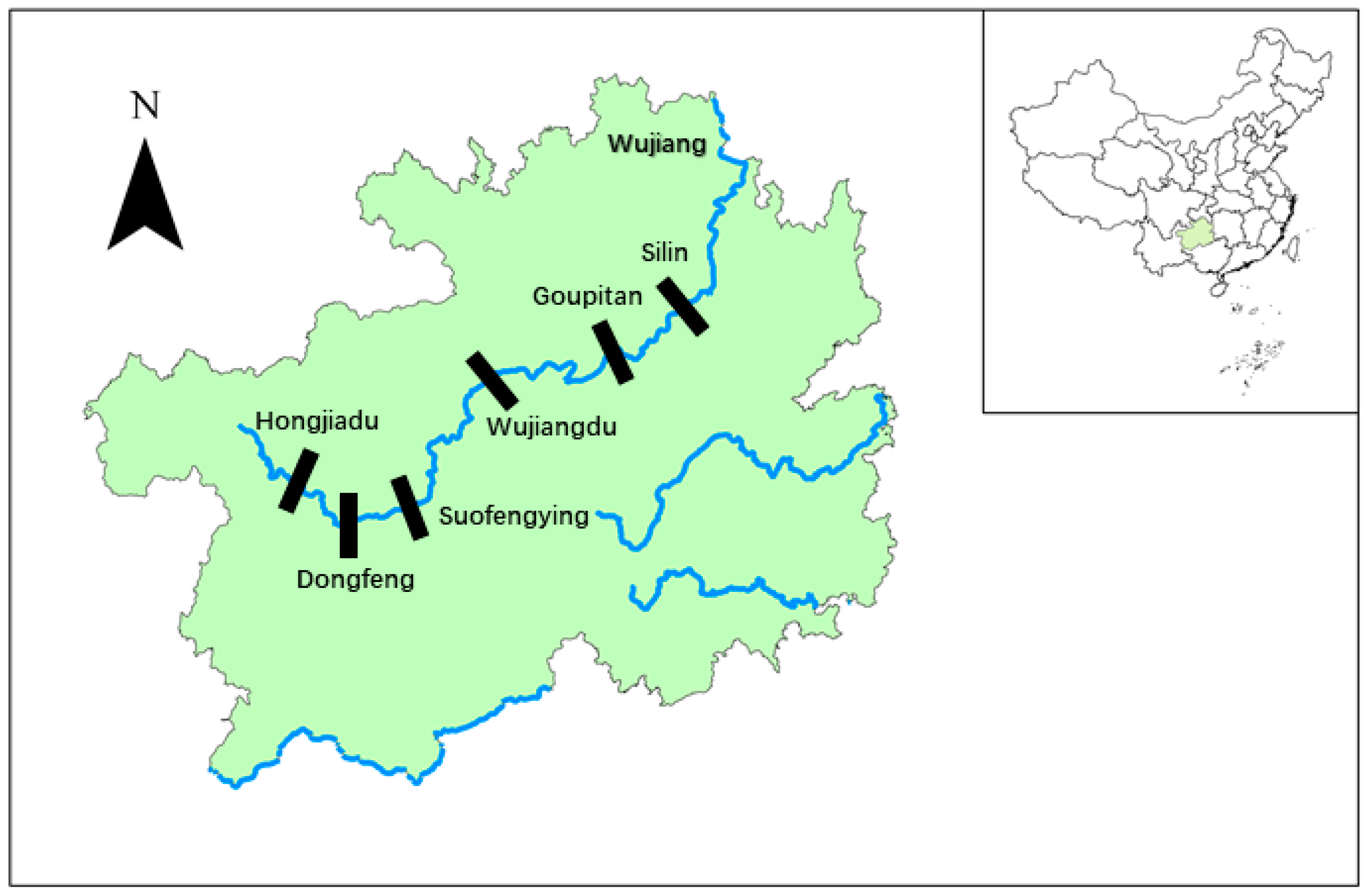
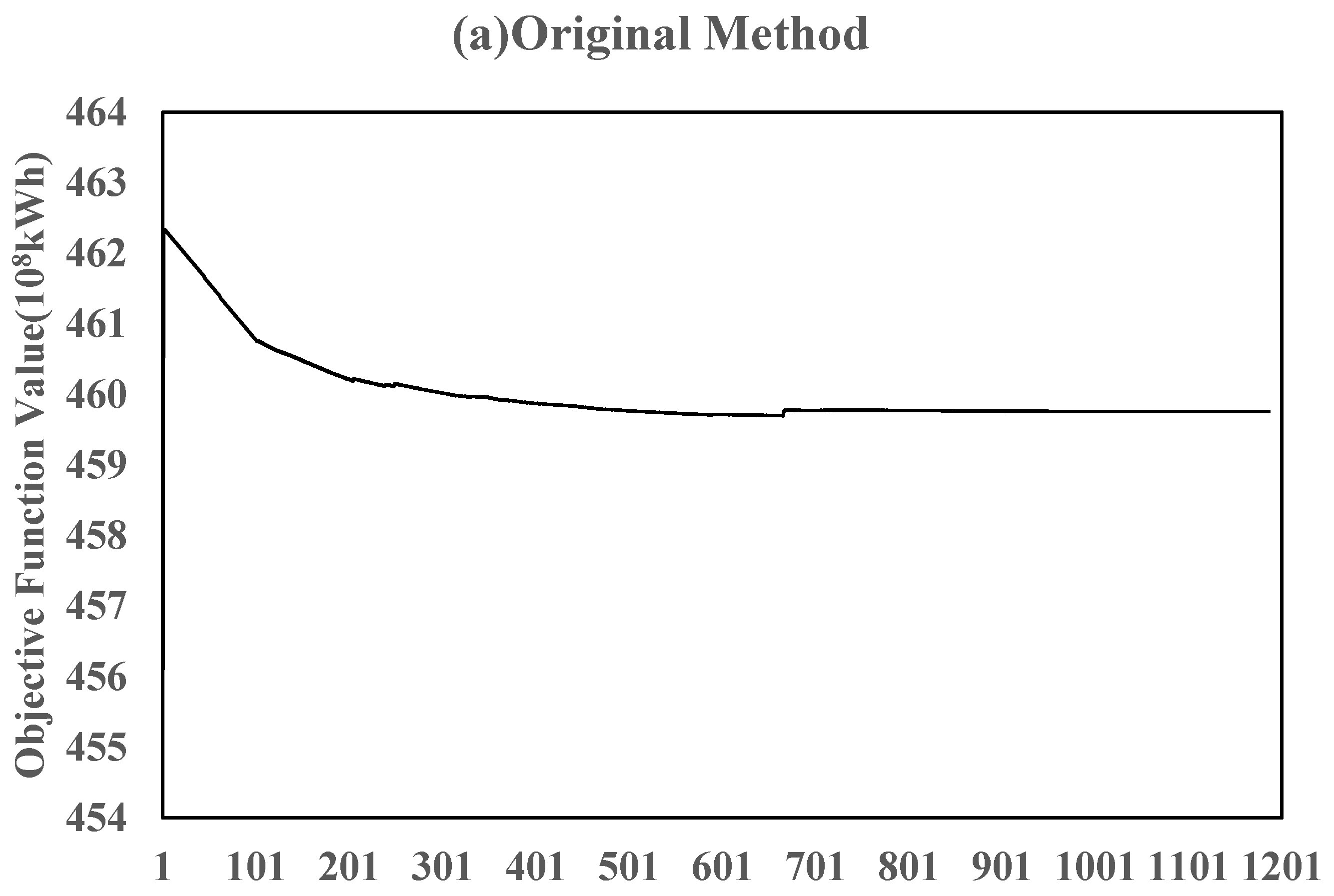
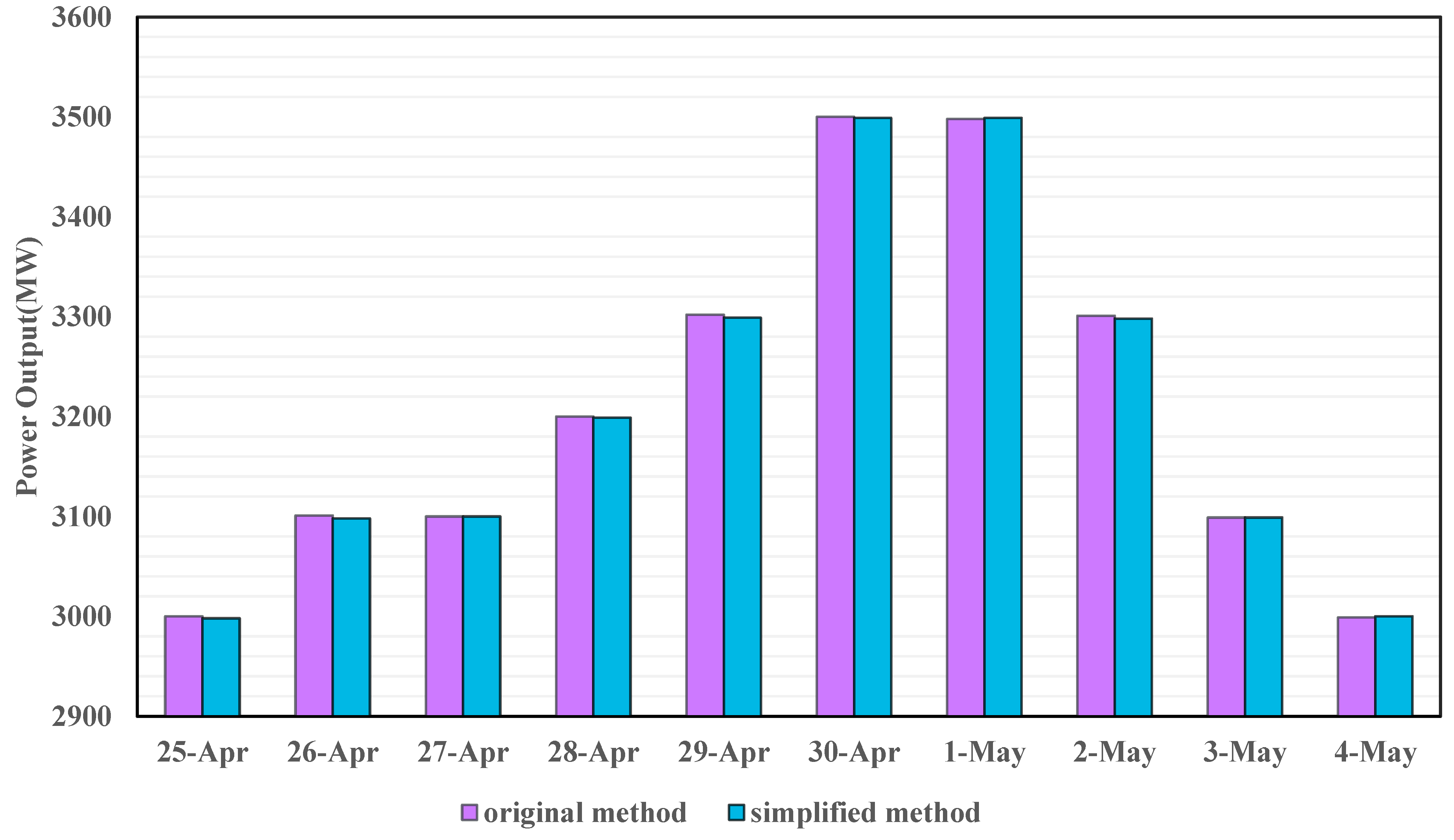
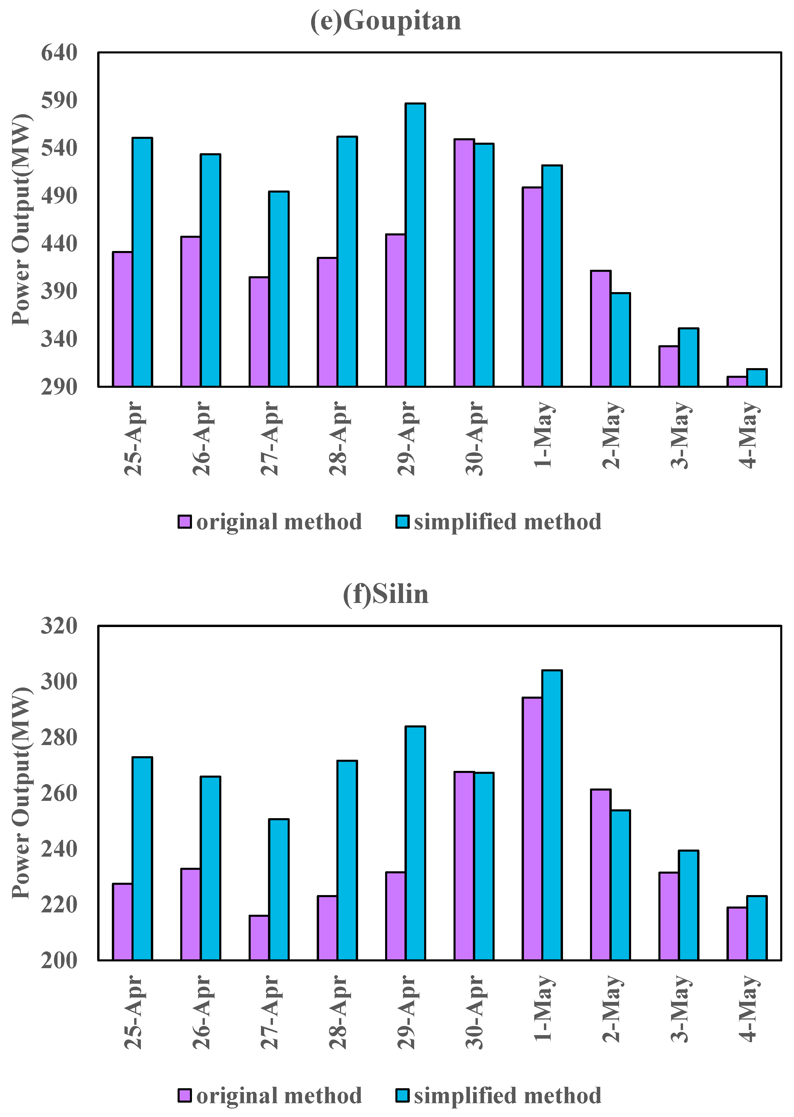
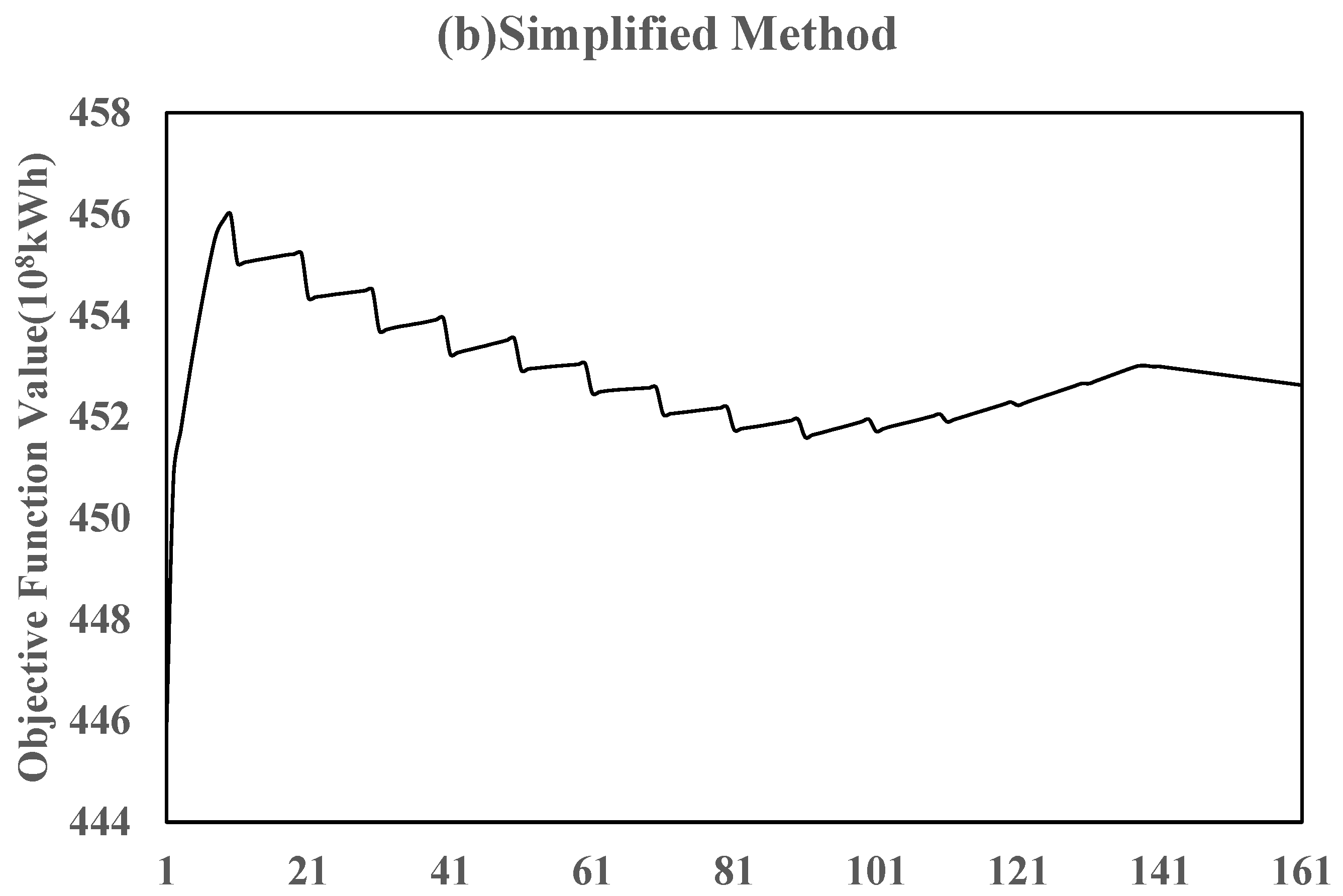
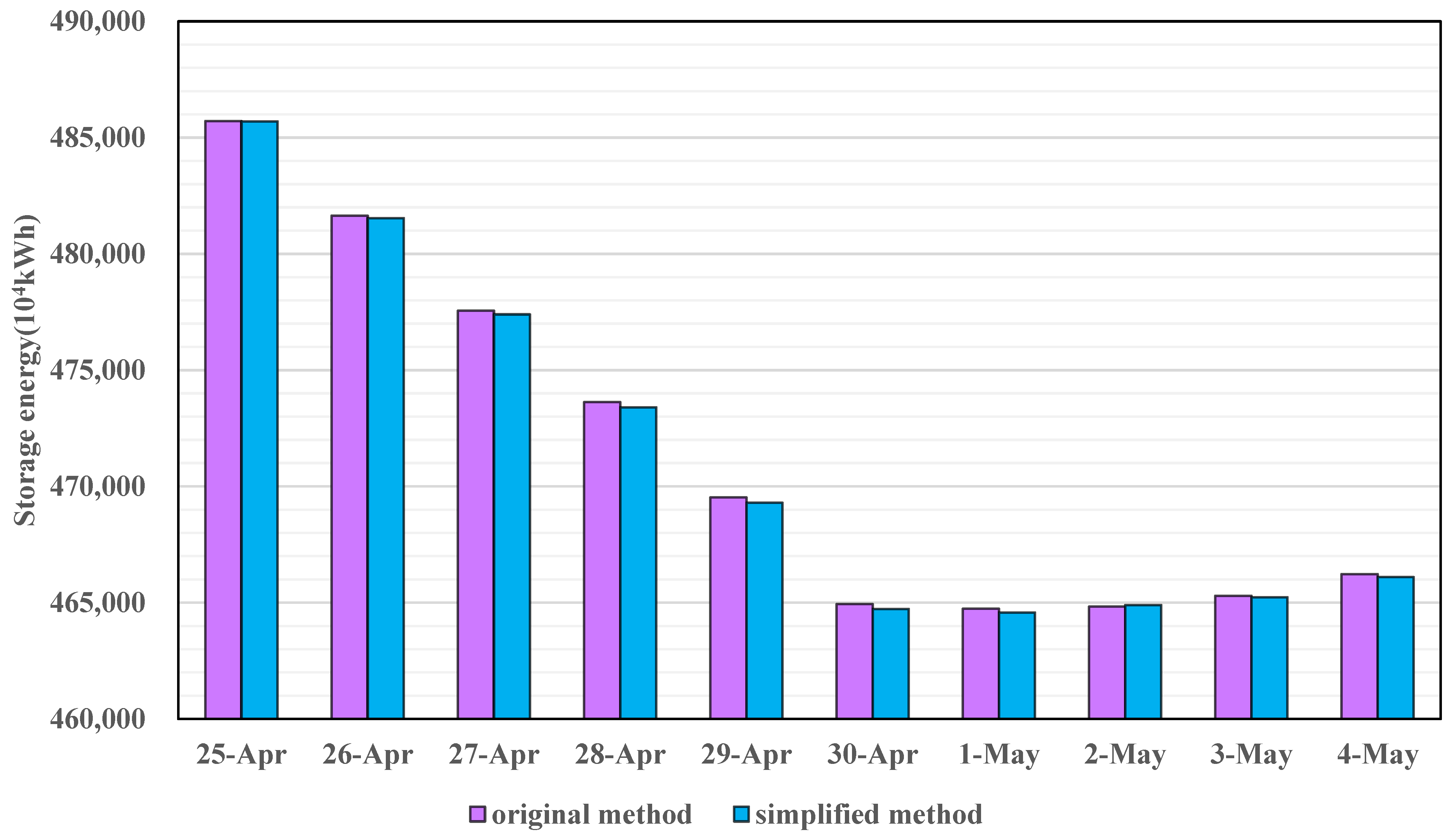
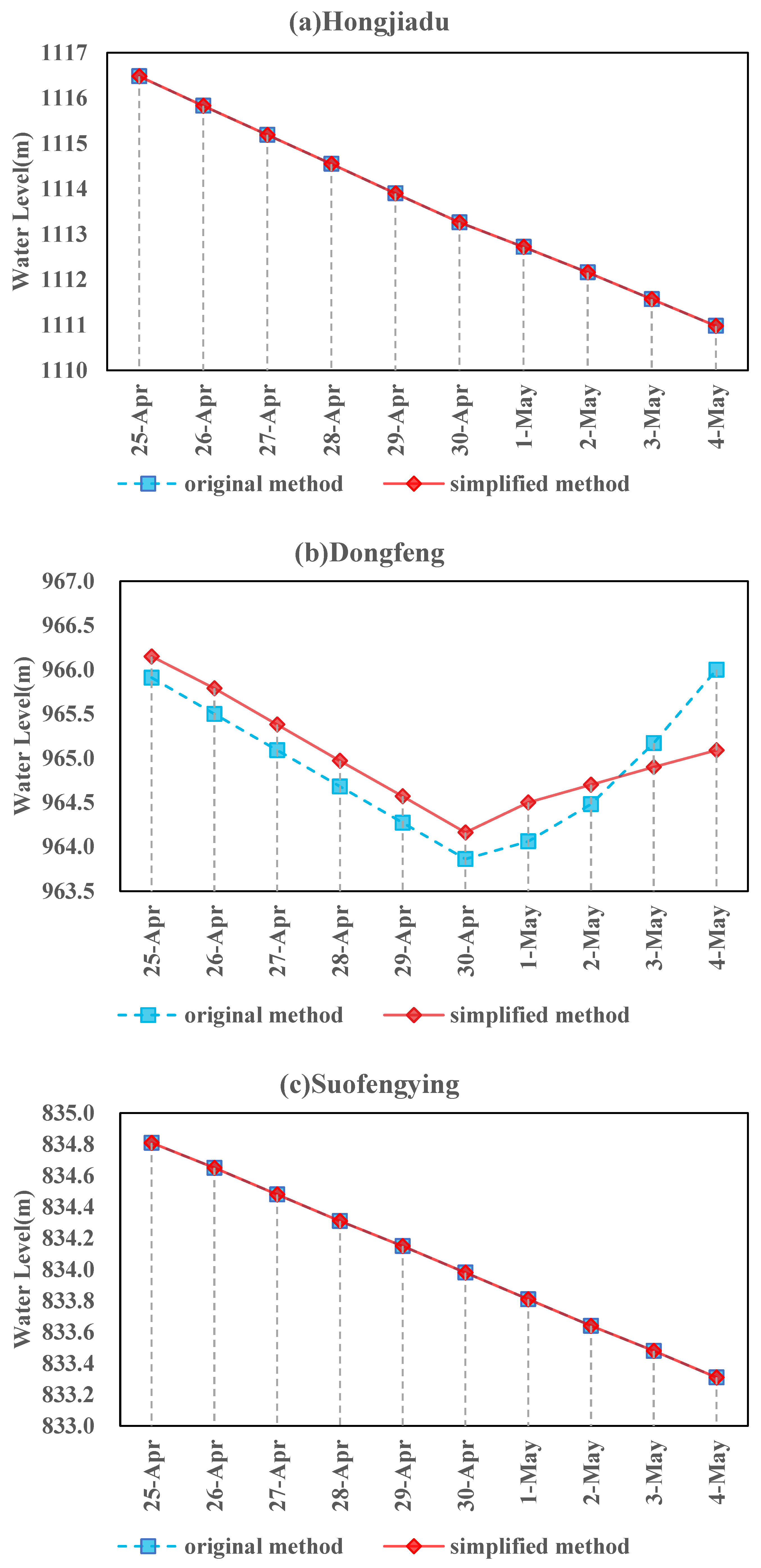
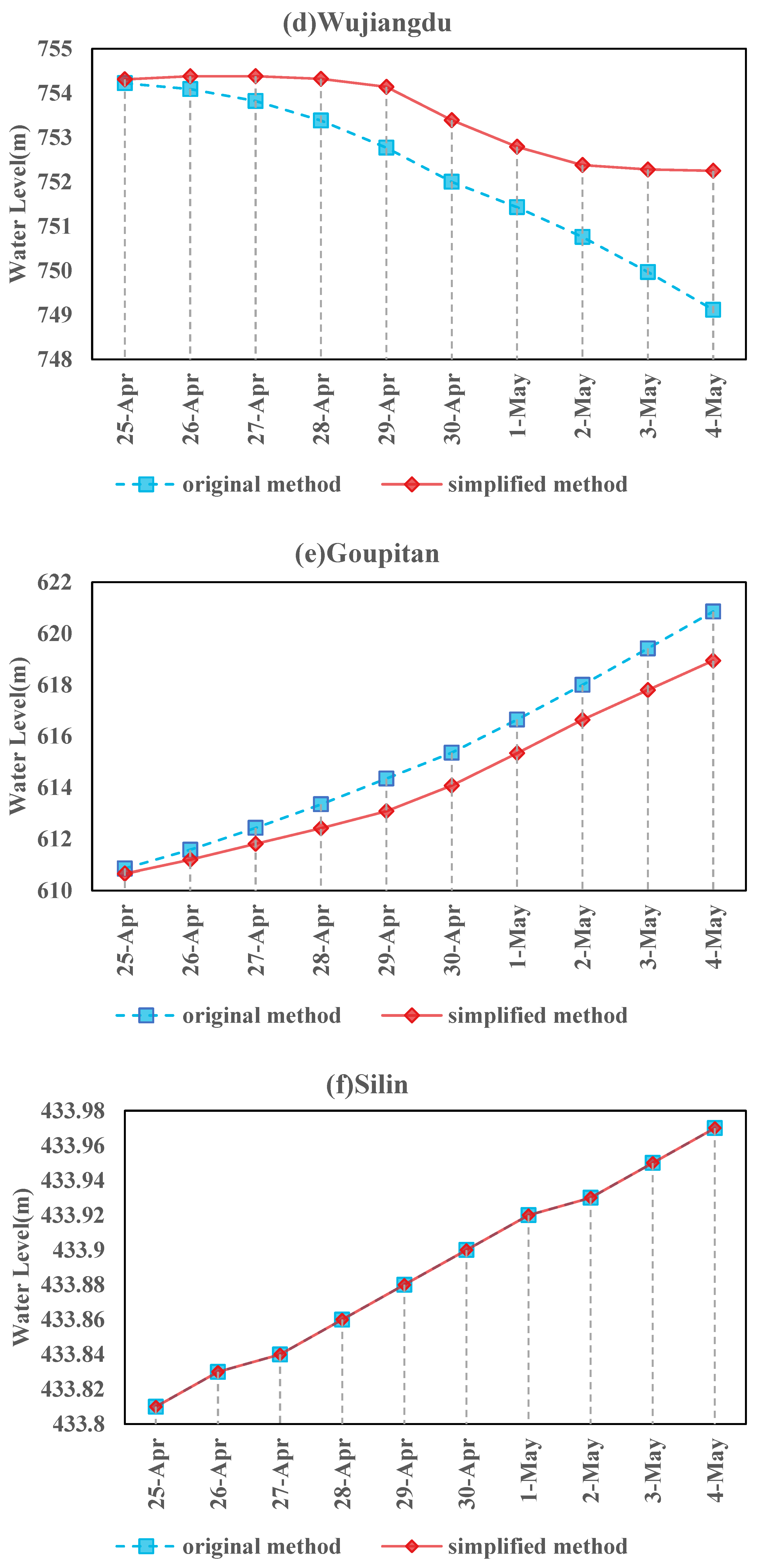
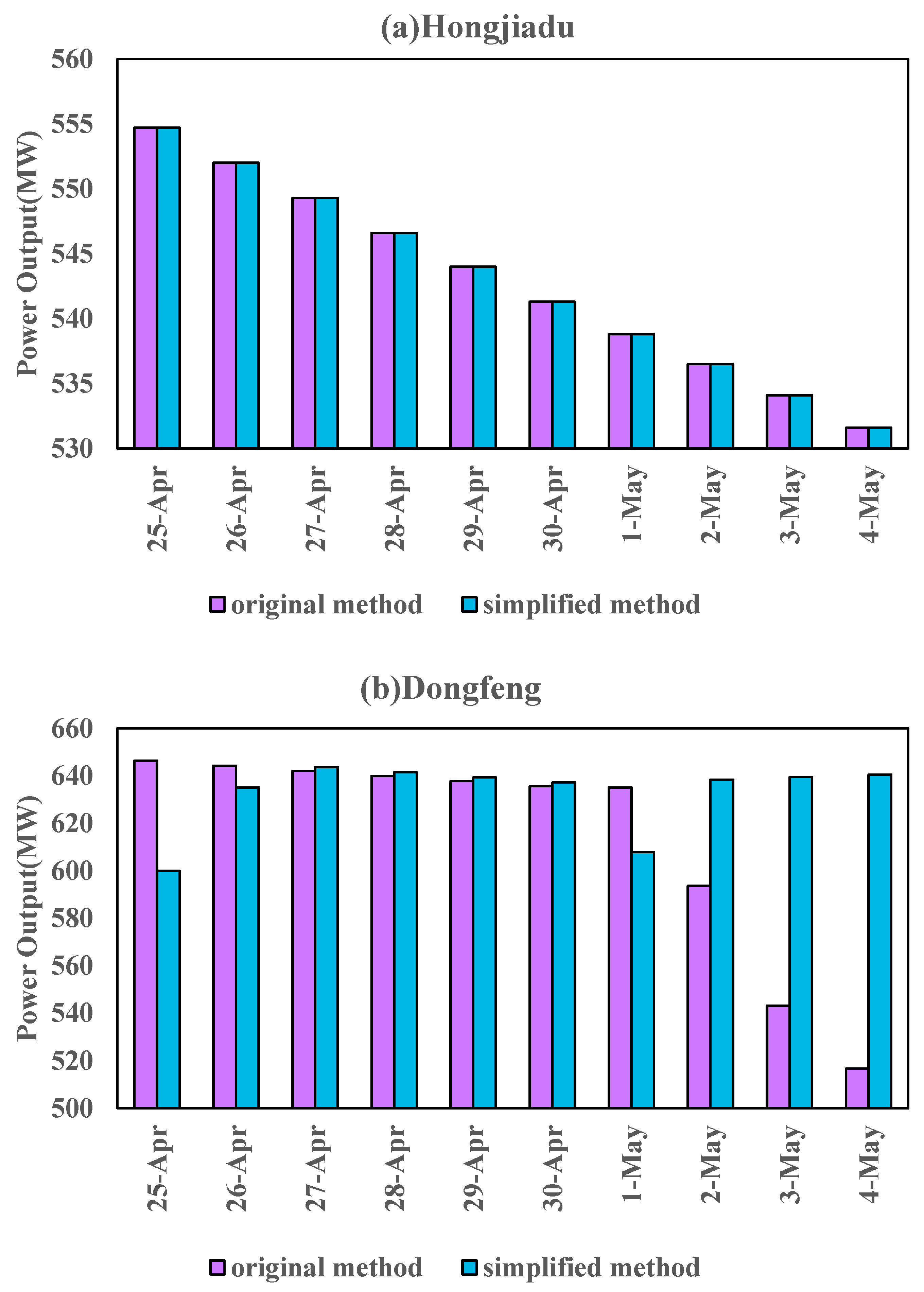
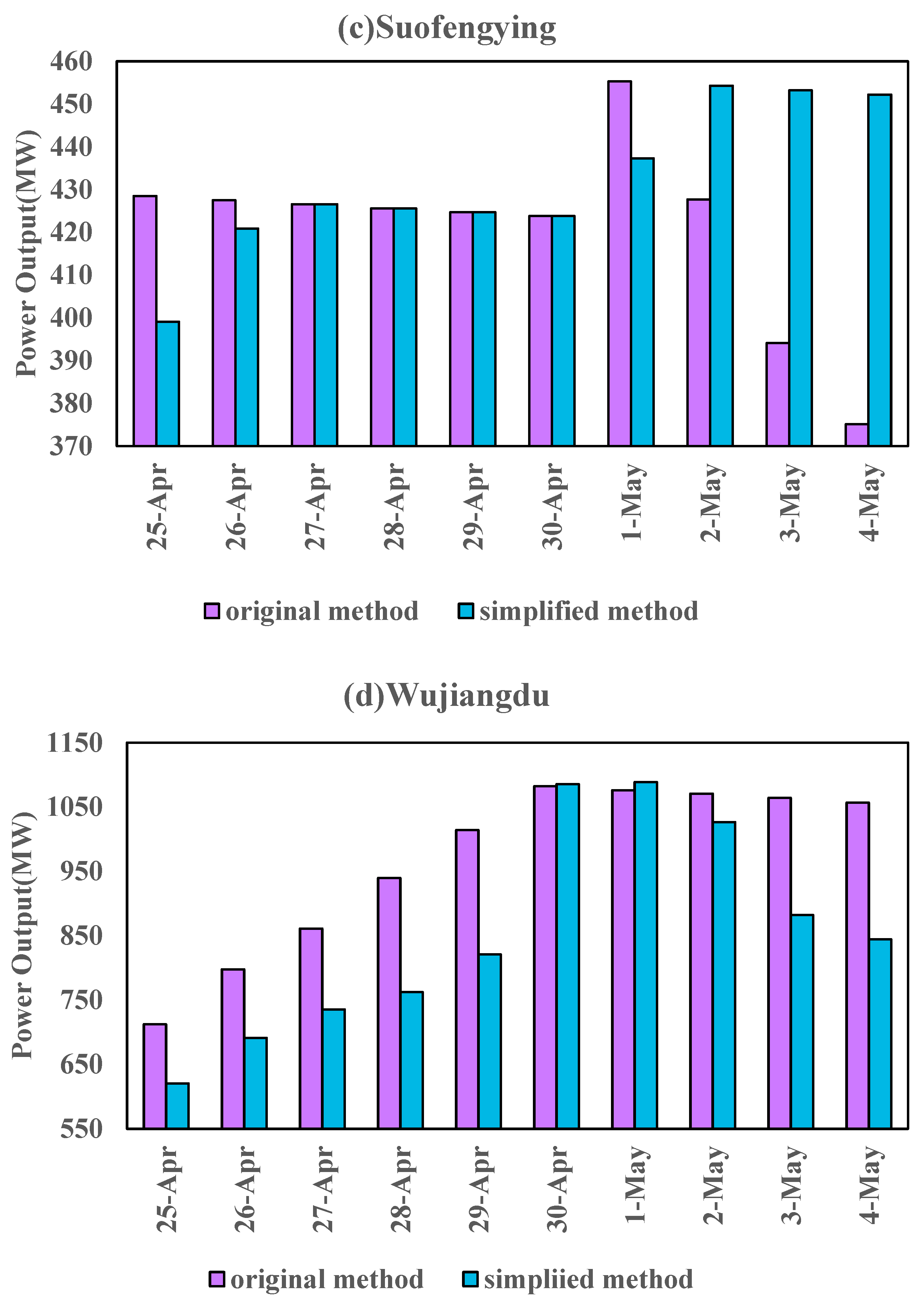
While solving the duality problem constructed by LR, the key point is the update iteration of the Lagrange multipliers. The subgradient method is often used, which searches along the direction of the subgradient to find the extreme point of the function. In this paper, the subgradient method is used to update multipliers. The calculation process for the simplified solution method is as follows:

Step 1: Initialize the Lagrange multiplier ${\gamma }^i,i=1$;

Step 2: Use DPSA to solve the mathematical model established in Section 2.1, where the object function is $F_3=F+\gamma \left\{\frac{1}{p}\ln {\displaystyle \sum }_{t=1}^T{e}^{P\left[f\left(t\right)-\underset{1\le t\le T}{\max }f\left(t\right)\right]}+\underset{1\le t\le T}{\max }f\left(t\right)\right\}-F_P$;

Step 3: Use the subgradient method to update the multiplier, ${\gamma }^{i+1}={\gamma }^i+{\mu }^i\times \left\{\frac{1}{p}\ln {\displaystyle \sum }_{t=1}^T{e}^{P\left[f\left(t\right)-\underset{1\le t\le T}{\max }f\left(t\right)\right]}+\underset{1\le t\le T}{\max }f\left(t\right)\right\}$, where ${\mu }^i$ is the update step of the Lagrange multiplier, set i = i + 1;

Step 4: Judge convergence: $\left|{\gamma }^{i+1}-{\gamma }^i\right|<\epsilon$, ${\displaystyle \sum }_{t=1}^T|{\displaystyle \sum }_{m=1}^M{P}_m^t-N^t|<\delta$ or i > I, where $\epsilon$ and $\delta$ are convergence precision, and δ represents the slight variation of the total load constraint error sum; I is the terminated iteration number. If convergence conditions are met, end the entire iterative process; otherwise, go to Step 2.

3. Case Study

The Wujiang River, known as Qianjiang in ancient times, is the longest tributary of the upper reaches of the Yangtze River in the south. It originates from the eastern foot of Wumeng Mountain in the northwest of Guizhou province and has two sources: Sancha River in the south and Liuchong River in the north. It flows through Yunnan, Guizhou, Hubei and Chongqing and finally empties into the Yangtze River in the north in the Fuling District of Chongqing. The main stream of the Wujiang River has a total length of 1037 km of which 802.1 km is in Guizhou, with a watershed area of 87,920 km² of which 66,849 km² is in Guizhou. It is the largest river in Guizhou. Most of the Wujiang River Basin belongs to the subtropical monsoon climate area, with abundant rainfall and uneven spatial and temporal distribution. The annual precipitation is over 1000 mm, mostly concentrated from May to October, accounting for more than 75% of the annual precipitation. The annual average runoff depth in the basin is 600 mm, higher than the national average of 271 mm and the Yangtze River average of 542 mm. Runoff is mainly rainwater replenishment, and its spatial and temporal distribution trends are basically consistent with that of precipitation. The annual runoff is 53.4 billion m³. Wujiang River is rich in water, stable runoff and small sediment content, which creates a good environment for the utilization of water resources. The natural drop in the Wujiang River Basin is concentrated, reaching 2124 m, with an average drop of 2.05‰. It is rich in water energy resources, and the theoretical reserve of the whole basin is 10,420 MW. At present, there are nine hydropower stations in Guizhou, including Hongjiadu, Dongfeng, Suofengying, Wujiangdu, Goupitan, Silin, Shatuo, Dahuashui and Geriqiao, with a total installed capacity of 8695 MW. This paper studies only six hydropower stations on the main stream of Wujiang River, named Hongjiadu, Dongfeng, Suofengying, Wujiangdu, Goupitan and Silin.

Table 1. Basic Parameters of Each Reservoir of Wujiang River.

Hydropower Plant	Regulation Performance	Installed Capacity (MW)	Dead Water Level (m)	Normal High Water Level (m)	Regulation Storage (108 m3)
Hongjiadu	Pluriennal Regulation	600	1076	1140	33.61
Dongfeng	Incomplete Annual Regulation	695	936	970	4.9
Suofengying	Daily Regulation	600	822	837	0.674
Wujiangdu	Incomplete Annual Regulation	1250	720	760	13.6
Goupitan	Pluriennal Regulation	3000	585	630	31.54
Silin	Daily Regulation	1050	431	440	3.17

shows the basic parameters of each reservoir of the Wujiang River. Figure 1 shows the location of each reservoir of the Wujiang cascaded hydropower system. Moreover, the mid-term optimization scheduling from 25 April 2022 to 4 May 2022 is studied in this paper. Then, the original solution method with Equation (12) and the simplified solution method with Equation (19) are applied to solve the medium-term, end-of-term storage energy maximization model and make a comparison; the solution process of the original solution method is similar to the simplified solution method.

When LR is adopted to solve end-of-term storage energy maximization model of medium-term scheduling, the Lagrange multiplier will be initialized. Furthermore, the Lagrange multiplier has a relatively clear physical meaning, that is, the change amount of storage energy of a cascaded hydropower system at the end of a scheduling term caused by the change of a unit output in the corresponding period. For a hydropower system consisting of several reservoirs, the Lagrange multipliers can be judged to be about 24 for the original solution method, which is hours in a single time period. Therefore, each initial component of the multiplier vector for the original solution method is set as 24. The update process of the subgradient method is divided into two stages in order to ensure good convergence and calculation. However, the simplified solution method converts the Lagrange dual problem with the multiple Lagrange multipliers to that with only a single Lagrange multiplier. Hence, the initial Lagrange multiplier of the simplified solution method can be set as 240, which is hours in the total scheduling term. And the update process of the Lagrange multiplier of the simplified solution method is similar to the original. Figure 2 shows the objective function value iteration process of the simplified method and the original method. The simplified method updates the Lagrange multipliers 35 times and iterates the objective function 161 times, taking 9 s in total. In contrast, the original method updates the Lagrange multipliers 493 times and iterates the objective function 1187 times, taking 30 s in total. The simplified method greatly improves the solution efficiency of the maximum end-of-term storage energy model at the medium-term scheduling, which is 70% shorter than the original method. This is because the simplified method has only one Lagrange multiplier, while the original method has ten Lagrange multipliers that need to be updated. In addition, in the original method, the Lagrange multipliers are related to each other, which makes the multiplier updating process long and leads to a slow solution speed. Figure 3 shows the power output process of the cascaded hydropower system for the original method and the simplified method. Figure 4 shows the storage energy process of the cascaded hydropower system for the original method and the simplified method. Compared with the original solution method, the maximum positive deviation of the output process of the cascaded hydropower system obtained by the simplified method is 1 MW, and the minimum negative deviation is −3 MW, and the deviation percentage is 0.10%. Moreover, compared with the original method, the maximum positive deviation of the cascaded hydropower system storage energy process obtained by the simplified method is 700,000 kWh, and the minimum negative deviation is −2.3 million kWh, and the deviation percentage is 0.05%. The end-of-term storage energy obtained by the original method is 4662.3 million kWh, while the end-of-term storage energy obtained by the simplified method is 4661 million kWh, which is reduced by 0.03%. So, it can be ignored. Therefore, the simplified method greatly improves the solution efficiency of the model and ensures the solution accuracy of the model. In the scheduling term, a given cascaded hydropower system load gradually increases and then decreases, with maximum cascaded hydropower system load demands occurring on April 30 and May 1. Therefore, the storage energy gradually decreases until May 1 in order to meet the cascaded hydropower system load demand. When the cascaded hydropower system load demand decreases, the storage energy will gradually increase to improve the regulating performance of the cascaded hydropower system after the scheduling term.

Figure 5 shows the water level process of each reservoir in the Wujiang cascaded hydropower system obtained by the simplified solution method and the original solution method. Figure 6 shows the power output process of each reservoir in the Wujiang cascaded hydropower system obtained by the simplified solution method and the original solution method. In addition, the tendency of the water level process of the simplified solution method is similar to that of the original solution method. In addition, the water level of the Hongjiadu, Suofengying and Wujiangdu hydropower plants gradually decreases, while that of the Goupitan and Silin hydropower plants increases gradually. In addition, the water level of the Dongfeng hydro plant decreases and then rises, which reaches the bottom on April 30. Through the comparison between the simplified solution method and the original solution method, the water level process of the Hongjiadu, Suofengying and Silin hydropower plants is the same. This is because the Suofengying and Silin hydropower plants are daily regulating reservoirs, which is equivalent to a runoff hydropower station in the medium-term scheduling. Moreover, the Hongjiadu hydropower plant is not only a leading reservoir but also a multiyear regulating reservoir, which plays an irreplaceable controlling role in the Wujiang cascaded hydropower system. There are huge differences in the water level process of the Dongfeng, Wujiangdu and Goupitan hydropower plants between the simplified solution method and the original solution method. In the simplified method, the water level of the Dongfeng hydropower plant is always higher than that in the original method before May 2; however, the end-of-term water level is 0.91 m lower than that in the original method. For the Wujiangdu hydropower plant, in the simplified solution method, the water level remains 754 m above, and the end-of-term water level is 752.52 m, which is 3.13 m higher than that in the original solution method. As for the Goupitan hydropower plant, in the simplified solution method, the water level is always lower than that in the original solution method, and the end-of-term water level is 1.91 m lower than that in the original method.

4. Discussion

In the case study, we show that the simplified solution method efficiently reduces the times of the Lagrange multiplier iteration update and subproblem iteration solution. In addition, the simplified solution method relaxes the system load demand for the total scheduling term instead of the multiple Lagrange multipliers for each scheduling period. Therefore, the simplified solution method avoids the interaction of the multiple Lagrange multipliers update for each scheduling period. However, the subproblem of the simplified solution method is solved with oscillation, while the subproblem of the original solution method is solved smoothly. Moreover, the Lagrange multiplier of the simplified solution method is convergent to 308.158, while the initial Lagrange multiplier is set as 240, varying greatly. In contrast, the Lagrange multipliers of the original solution method are convergent to 24.543, while the initial Lagrange multipliers are set as 24, changing a little. Therefore, the simplified solution method is less stable than the original. And the interaction of each scheduling period was inherently included in the Lagrange multiplier update process of the simplified solution method, which causes the change of the Lagrange multiplier to be greater; the range of the Lagrange multiplier of the simplified solution method is between 240 and 360.

5. Conclusions

The end-of-term storage energy maximization model is in general solved by LR. This paper proposes a simplified solution method based on LR and the aggregate function method for an end-of-term storage energy maximization model with only one Lagrange multiplier. Then, the simplified solution method adopts DPSA to solve the subproblem and the subgradient method to update the Lagrange multiplier. In addition, the Wujiang cascaded hydropower system is studied. The results show that the solution time of the simplified solution method is 70% shorter than that of the original solution method, which greatly improves the solution efficiency; the end-of-term storage energy obtained by the simplified solution method is reduced by 0.03% compared with the original solution method, which ensures the solution accuracy.

Future Possible Work

The simplified solution method based on LR and the aggregate function method could be extended to solve the hydropower system optimal operation model with complicated side constraints in which the complex side constraints could be converted to a maximum form, such as minimum power decision constraints and system load demand constraints. In later research work, more and more efficient Lagrange multiplier iterative update method with heuristic algorithms will be applied to simplify the solution process and alleviate the Lagrange multiplier iterative oscillation. Moreover, it could be applied in what could be solved by LR to convert multiple constraints to a total constraint in other areas. In the future, the optimal goal is to investigate how to meet system load demand given as the installed capacity of new energy gradually increases. The simplified solution method provides a possible way to solve the cascaded hydropower system load balance problem efficiently.

References

1. Zeng, M.; Zhang, K.; Liu, D. Overall review of pumped-hydro energy storage in China: Status quo, operation mechanism and policy barriers. Renew. Sustain. Energy Rev. 2013, 17, 35–43. [Google Scholar] [CrossRef]
2. Shang, Y.; Lu, S.; Ye, Y.; Liu, R.; Shang, L.; Liu, C.; Meng, X.; Li, X.; Fan, Q. China’ energy-water nexus: Hydropower generation potential of joint operation of the Three Gorges and Qingjiang cascade reservoirs. Energy 2018, 142, 14–32. [Google Scholar] [CrossRef]
3. Wu, X.; Cheng, C.; Zeng, Y.; Lund, J.R. Centralized versus Distributed Cooperative Operating Rules for Multiple Cascaded Hydropower Reservoirs. J. Water Resour. Plan. Manag. 2016, 142, 05016008. [Google Scholar] [CrossRef]
4. Liao, S.; Liu, H.; Liu, Z.; Liu, B.; Li, G.; Li, S. Medium-term peak shaving operation of cascade hydropower plants considering water delay time. Renew. Energy 2021, 179, 406–417. [Google Scholar] [CrossRef]
5. Labadie, J.W. Optimal Operation of Multireservoir Systems: State-of-the-Art Review. J. Water Resour. Plan. Manag. 2004, 130, 93–111. [Google Scholar] [CrossRef]
6. Yeh, W.W.-G. Reservoir Management and Operations Models: A State-of-the-Art Review. Water Resour. Res. 1985, 21, 1797–1818. [Google Scholar] [CrossRef]
7. Yoo, J.-H. Maximization of hydropower generation through the application of a linear programming model. J. Hydrol. 2009, 376, 182–187. [Google Scholar] [CrossRef]
8. Barros, M.T.L.; Tsai, F.T.-C.; Yang, S.-L.; Lopes, J.E.G.; Yeh, W.W.-G. Optimization of Large-Scale Hydropower System Operations. J. Water Resour. Plan. Manag. 2003, 129, 178–188. [Google Scholar] [CrossRef]
9. Cheng, C.-T.; Liao, S.-L.; Tang, Z.-T.; Zhao, M.-Y. Comparison of particle swarm optimization and dynamic programming for large scale hydro unit load dispatch. Energy Convers. Manag. 2009, 50, 3007–3014. [Google Scholar] [CrossRef]
10. Feng, Z.-K.; Niu, W.-J.; Cheng, C.-T.; Wu, X.-Y. Optimization of large-scale hydropower system peak operation with hybrid dynamic programming and domain knowledge. J. Clean. Prod. 2018, 171, 390–402. [Google Scholar] [CrossRef]
11. Zhao, T.; Zhao, J.; Yang, D. Improved Dynamic Programming for Hydropower Reservoir Operation. J. Water Resour. Plan. Manag. 2014, 140, 365–374. [Google Scholar] [CrossRef]
12. Oliveira, R.; Loucks, D.P. Operating rules for multireservoir systems. Water Resour. Res. 1997, 33, 839–852. [Google Scholar] [CrossRef]
13. Kumar, D.N.; Reddy, M.J. Multipurpose Reservoir Operation Using Particle Swarm Optimization. J. Water Resour. Plan. Manag. 2007, 133, 192–201. [Google Scholar] [CrossRef]
14. Kumar, D.N.; Reddy, M.J. Ant Colony Optimization for Multi-Purpose Reservoir Operation. Water Resour. Manag. 2006, 20, 879–898. [Google Scholar] [CrossRef]
15. Giles, J.E.; Wunderlich, W.O. Weekly Multipurpose Planning Model for TVA Reservoir System. J. Water Resour. Plan. Manag. Div. 1981, 107, 495–511. [Google Scholar] [CrossRef]
16. Trott, W.J.; Yeh, W.W.-G. Optimization of Multiple Reservoir System. J. Hydraul. Div. 1973, 99, 1865–1884. [Google Scholar] [CrossRef]
17. Opan, M. Irrigation-energy management using a DPSA-based optimization model in the Ceyhan Basin of Turkey. J. Hydrol. 2010, 385, 353–360. [Google Scholar] [CrossRef]
18. Zhang, W.; Liu, P.; Chen, X.; Wang, L.; Ai, X.; Feng, M.; Liu, D.; Liu, Y. Optimal Operation of Multi-reservoir Systems Considering Time-lags of Flood Routing. Water Resour. Manag. 2015, 30, 523–540. [Google Scholar] [CrossRef]
19. He, Z.; Wang, C.; Wang, Y.; Wei, B.; Zhou, J.; Zhang, H.; Qin, H. Dynamic programming with successive approximation and relaxation strategy for long-term joint power generation scheduling of large-scale hydropower station group. Energy 2021, 222, 119960. [Google Scholar] [CrossRef]
20. Fisher, M.L. The Lagrangian Relaxation Method for Solving Integer Programming Problems. Manag. Sci. 1981, 27, 1–18. [Google Scholar] [CrossRef]
21. Fisher, M.L. An Applications Oriented Guide to Lagrangian Relaxation. Interfaces 1985, 15, 10–21. [Google Scholar] [CrossRef]
22. Guan, X.; Ni, E.; Li, R.; Luh, P.B. An optimization-based algorithm for scheduling hydrothermal power systems with cascaded reservoirs and discrete hydro constraints. IEEE Trans. Power Syst. 1997, 12, 1775–1780. [Google Scholar] [CrossRef] [Green Version]
23. Redondo, N.J.; Conejo, A. Short-term hydro-thermal coordination by Lagrangian relaxation: Solution of the dual problem. IEEE Trans. Power Syst. 1999, 14, 89–95. [Google Scholar] [CrossRef]
24. Soares, S.; Ohishi, T.; Cicogna, M.; Arce, A. Dynamic dispatch of hydro generating units. In Proceedings of the 2003 IEEE Bologna Power Tech Conference Proceedings, Bologna, Italy, 23–26 June 2003; Volume 2, p. 6. [Google Scholar]
25. Zhai, Q.; Guan, X.; Cui, J. Unit commitment with identical units successive subproblem solving method based on Lagrangian relaxation. IEEE Trans. Power Syst. 2002, 17, 1250–1257. [Google Scholar] [CrossRef]
26. Finardi, E.C.; Scuzziato, M.R. A comparative analysis of different dual problems in the Lagrangian Relaxation context for solving the Hydro Unit Commitment problem. Electr. Power Syst. Res. 2014, 107, 221–229. [Google Scholar] [CrossRef]
27. Pursimo, J.; Antila, H.; Vilkko, M.; Lautala, P. A short-term scheduling for a hydropower plant chain. Int. J. Electr. Power Energy Syst. 1998, 20, 525–532. [Google Scholar] [CrossRef]
28. Wang, J. Short-term generation scheduling model of Fujian hydro system. Energy Convers. Manag. 2009, 50, 1085–1094. [Google Scholar] [CrossRef]
29. Finardi, E.; Takigawa, F.; Brito, B. Assessing solution quality and computational performance in the hydro unit commitment problem considering different mathematical programming approaches. Electr. Power Syst. Res. 2016, 136, 212–222. [Google Scholar] [CrossRef]
30. Liu, B.; Cheng, C.; Wang, S.; Liao, S.; Chau, K.-W.; Wu, X.; Li, W. Parallel chance-constrained dynamic programming for cascade hydropower system operation. Energy 2018, 165, 752–767. [Google Scholar] [CrossRef]
31. Liu, P.; Guo, S.; Xu, X.; Chen, J. Derivation of Aggregation-Based Joint Operating Rule Curves for Cascade Hydropower Reservoirs. Water Resour. Manag. 2011, 25, 3177–3200. [Google Scholar] [CrossRef]
32. Li, X. An entropy-based aggregate method for minimax optimization. Eng. Optim. 1992, 18, 277–285. [Google Scholar] [CrossRef]
Figure 1. The Location of Each Reservoir of Wujiang Cascaded Hydropower System.
Energies 15 04503 g001
Figure 2. Objective Function Value Iteration Process of Original Method and Simplified Method.
Energies 15 04503 g002aEnergies 15 04503 g002b
Figure 3. Power Output Process of Cascaded Hydropower System Obtained by Original Method and Simplified Method.
Energies 15 04503 g003
Figure 4. Storage Energy Process of Cascaded Hydropower System Obtained by Original Method and Simplified Method.
Energies 15 04503 g004
Figure 5. The Water Level Process of Each Reservoir in Wujiang River Obtained by the Simplified Solution Method and the Original Solution Method.
Energies 15 04503 g005aEnergies 15 04503 g005b
Figure 6. The Power Output Process of Each Reservoir in Wujiang River Obtained by the Simplified Solution Method and the Original Solution Method.
Energies 15 04503 g006aEnergies 15 04503 g006bEnergies 15 04503 g006c