Article

Application of Machine Learning for Lithofacies Prediction and Cluster Analysis Approach to Identify Rock Type

1
Institute of Geophysics and Geomatics, China University of Geosciences, Wuhan 430074, China
2
Institute for Ecological Research and Pollution Control of Plateau Lakes, School of Ecology and Environmental Science, Yunnan University, Kunming 650500, China
3
Department of Geological Resources and Engineering, Faculty of Earth Resources, China University of Geosciences, Wuhan 430074, China
4
State Key Laboratory of Geomechanics and Geotechnical Engineering, Institute of Rock and Soil Mechanics, Chinese Academy of Sciences, Wuhan 430071, China
5
University of Chinese Academy of Sciences, Beijing 100049, China
*
Author to whom correspondence should be addressed.
Energies 2022, 15(12), 4501; https://doi.org/10.3390/en15124501
Submission received: 11 May 2022 / Revised: 17 June 2022 / Accepted: 18 June 2022 / Published: 20 June 2022

Abstract

:
Nowadays, there are significant issues in the classification of lithofacies and the identification of rock types in particular. Zamzama gas field demonstrates the complex nature of lithofacies due to the heterogeneous nature of the reservoir formation, while it is quite challenging to identify the lithofacies. Using our machine learning approach and cluster analysis, we can not only resolve these difficulties, but also minimize their time-consuming aspects and provide an accurate result even when the user is inexperienced. To constrain accurate reservoir models, rock type identification is a critical step in reservoir characterization. Many empirical and statistical methodologies have been established based on the effect of rock type on reservoir performance. Only well-logged data are provided, and no cores are sampled. Given these circumstances, and the fact that traditional methods such as regression are intractable, we have chosen to apply three strategies: (1) using a self-organizing map (SOM) to arrange depth intervals with similar facies into clusters; (2) clustering to split various facies into specific zones; and (3) the cluster analysis technique is used to identify rock type. In the Zamzama gas field, SOM and cluster analysis techniques discovered four group of facies, each of which was internally comparable in petrophysical properties but distinct from the others. Gamma Ray (GR), Effective Porosity(eff), Permeability (Perm) and Water Saturation (Sw) are used to generate these results. The findings and behavior of four facies shows that facies-01 and facies-02 have good characteristics for acting as gas-bearing sediments, whereas facies-03 and facies-04 are non-reservoir sediments. The outcomes of this study stated that facies-01 is an excellent rock-type zone in the reservoir of the Zamzama gas field.

1. Introduction

Machine learning emerged as a subfield of artificial intelligence (AI) in the second decade of the twentieth century, using self-learning algorithms that gathered information from data to make predictions [1,2,3,4]. Machine learning offers a more efficient option to capture the information in data to gradually improve the performance of prediction models and make data-driven decisions [5,6,7,8], rather than needing humans to manually create rules and build models from analyzing massive volumes of data [9,10,11]. Machine learning is divided into three categories: supervised learning, unsupervised learning, and reinforcement learning [12,13]. Each type has its application and algorithm; however, because of the lack of outcome information in our case study, we primarily focused on unsupervised learning. Furthermore, unsupervised learning takes into account the fact that it may automatically extract hidden patterns without human instruction, making it more similar to machine learning than other varieties [14]. We used a machine learning model to categorize the facies for Zamzama gas field and tested the findings against real facies data in this study. Our model likewise uses data from this field, but we used a novel model called the self-organizing map (SOM) to tackle the problem [15]. In the situation of a lack of facies data or geologically inexperienced users, our model would be the best fit [16]. The principal component analysis (PCA) is our model’s first unsupervised learning approach [17]. This is a linear mathematical strategy for condensing a big set of variables (seismic characteristics) into a smaller set that retains the majority of the independent information variation found in the larger data set [18,19]. One can distinguish sedimentary units with similar log characteristics by gathering data from several good logs [20,21,22,23,24]. In the literature, sedimentary units established on this basis and characterized from wireline logs were referred to as electrofacies or logfacies [17,25,26,27]. One of the most accurate and impactful procedures in oil-bearing clastic reservoirs is multivariate cluster analysis (referred to as the best method of data grouping in the literature) [8,16].
The aim of this research is to classify gamma-ray, porosity, permeability and water saturation into logfacies and rock types. Our study compares and evaluates lithofacies and various rock type identifications, utilizing SOM and cluster analysis, via hierarchical and non-hierarchical approaches to calibrate the appropriate model for researching lithofacies and rock-type identification. The rock type classification is performed using the cluster analysis method, which aims to discover groups of well-log data with similar characteristics. This classification is based on the unique properties of well-log measurements, which reflect lithofacies within the recorded interval, and does not require any artificial segmentation of the data population [28].
A cluster analysis can be performed using a variety of methods. Furthermore, unsupervised learning is more similar to machine learning than other forms since it can automatically extract hidden patterns without human assistance [29,30,31]. For lithofacies classification, there is an unsupervised learning model called support vector machine (SVM). The SVM is a useful approach for higher-dimensional datasets that is also versatile, as alternative kernels can be specified according to the user’s needs. The SOM is the next step in the process. There are massive data analysis challenges, particularly in the classification of lithofacies and the identification of rock types, both of which generate large amounts of data, as well as the fact that humans are unable to fully appreciate the link between seismic properties [32]. Using the advanced machine learning approach and cluster analysis, we can not only solve these problems, but also reduce their time-consuming nature, and deliver an accurate result even when the user is unskilled. Finally, clustering is used to classify subgroups (facies) based on their dissimilarity. In this research, we want to systematize the essential background of the SOM and then apply this workflow to facies classification in two real examples. Based on the final results, which are compared, several discussions are presented of lithofacies identification.

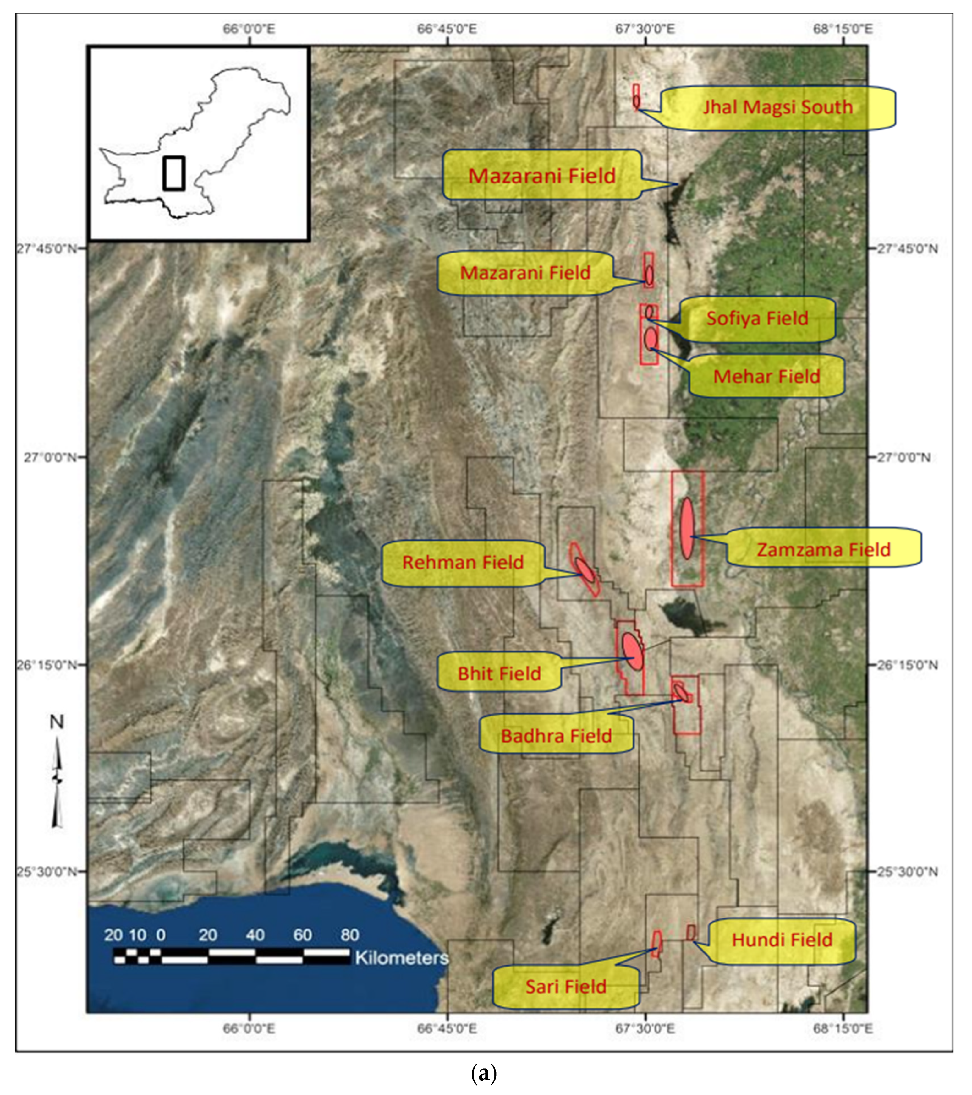
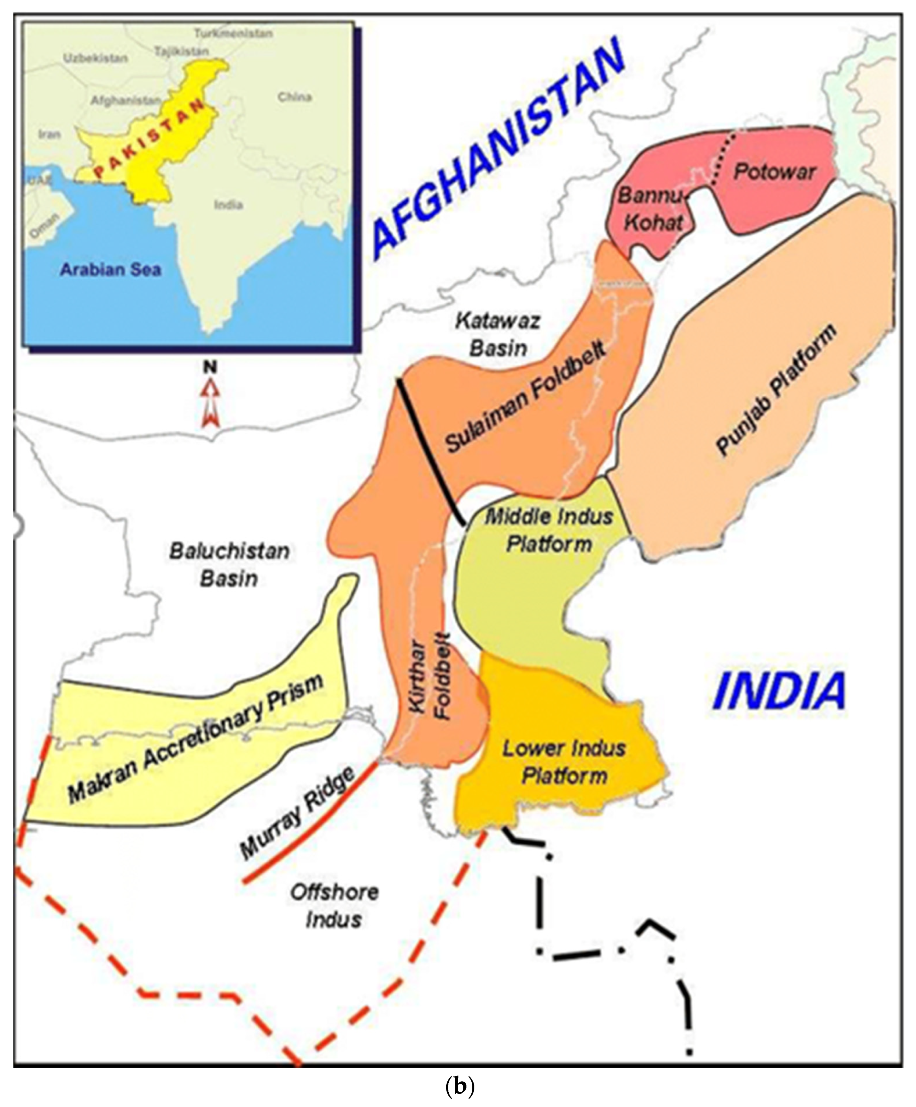
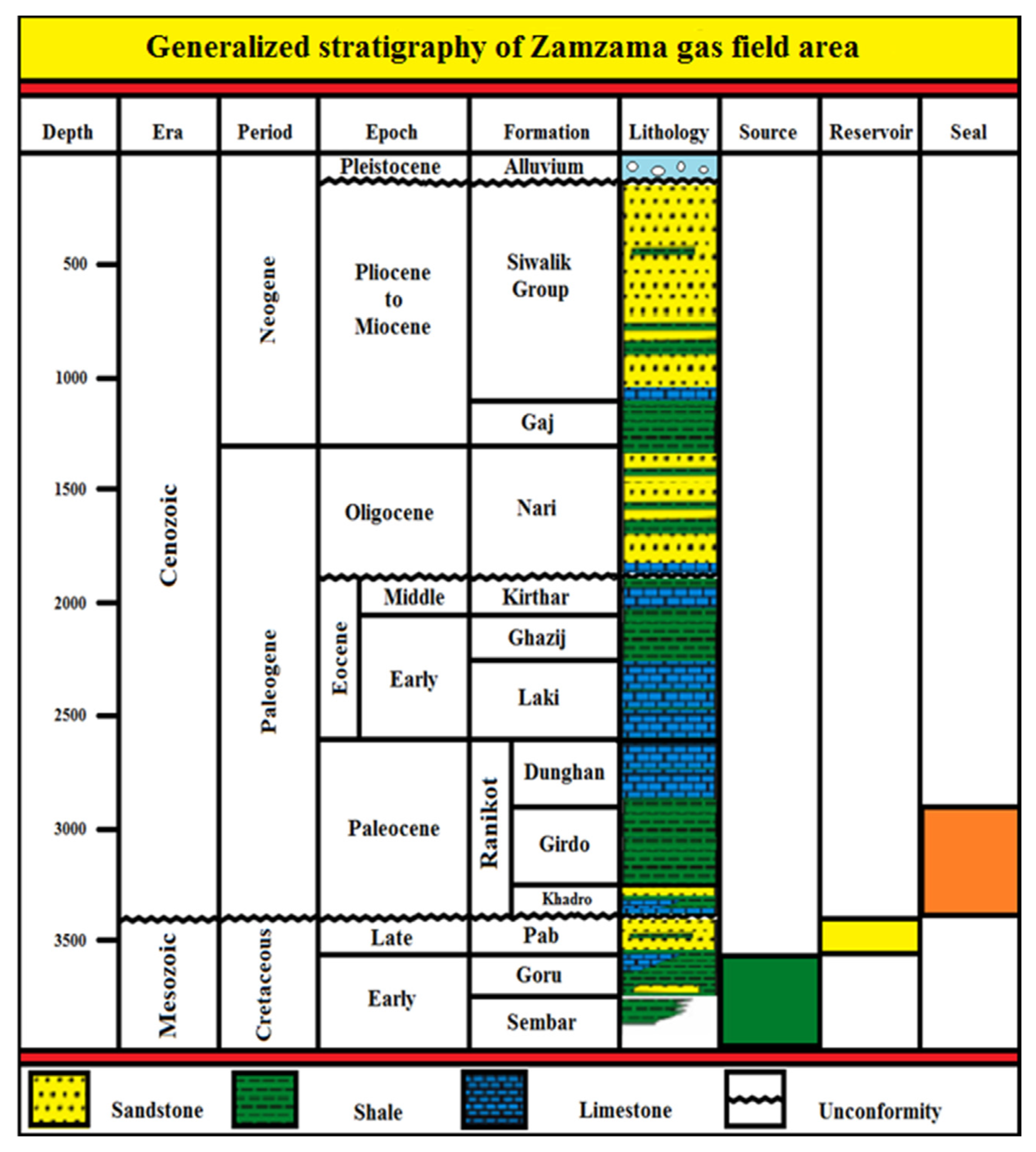
General Geology and Stratigraphy of the Study Area

The Zamzama gas field is located on the eastern edge of the Kirthar Foldbelt and is a broad, trust-related anticline northeast of the fields of Bhit and Badhra, and south of the fields of Mehar, Sofiya, and Mazarani (Figure 1a). In the frontal folds on the Kirthar foredeep, these field are situated along the western edge of the Lower Indus Basin [33,34]. The Zamzama gas area is situated along the Kirthar folds and thrust belts of Pakistan’s Southern Indus Basin. The southern Indus Basin is limited by the Indian Shield to the east and the Indian plate’s marginal zone to the west, as well as the Sukkur rift from the north to the offshore Indus in the south [35,36]. The Kirthar Foldbelt in Pakistan is part of the lateral mountain belt linking Makran’s accretionary wedge to the Himalayan orogeny. Parallel to the regional plate motion vector, the area is undergoing oblique deformation (Figure 1b). In 1998, with estimated wet gas in place at discovery, the Zamzama Field was discovered and has provided condensate cumulatively to date [25,26].
Most of the production comes from late Cretaceous Pab Formation fluvial and shallow marine sandstones, but the Zamzama area also produces sandstones from the estuarine Palaeocene Khadro formation, which are from the Pab formation in stratigraphic pressure isolation. In the Zamzama region, the Sembar’s Cretaceous shales and the Goru formations are regarded as the principal source rock [37,38,39,40]. Through a majority of the Southern Indus Basin, the Sembar Formation was deposited in marine settings [41,42,43]. The Lower Goru Formation was deposited over the whole basin of the Southern Indus [33,37]. The early Cretaceous Goru Formation, which is divided into two sections (the Lower Goru Formation (LGF) and Upper Goru Formation (UGF)), superimposes the Sembar Formation [44,45]. The Goru Formation was accumulated in a shallow marine environment such as a shoreface to the fluvial-based proximal delta-front depositional framework [1,41]. Quite coarse to fine, porous, and permeable sediments are preserved in fluvial networks and create reservoirs in fluvial-based depositional systems [9,37,39]. The Lower Goru Formation, which includes quite coarse to fine sediments, is the largest reservoir rock in the Lower Indus Basin [33,34]. However, in our study area, Goru formation is acting as a source rock, while Pab sandstone is the main reservoir rock within the Zamzama gas field (Figure 2). The main producing reservoir in the Zamzama gas field is the Maastrichtian Pab Formation, which shows the deposition of the sand-rich fluvio-deltaic coastal plain and shoreface depositional system that passes westwards into deep marine turbidites. An alternative target is sandstone reservoirs within the underlying Palaeocene Khadro Formation, which are separated by varied thicknesses of coastal plain shales and mudstones, across the top Pab Formation unconformity. The Khadro Formation sandstones are made up of estuary, intertidal, and shoreface deposits, with the shoreface units cut by tidal channels, and are hence very discontinuous and variable in distribution. The Palaeocene Girdo (Ranikot) Formation marine shales serve as the top seal for the Khadro Formation reservoir sand, which is present throughout the field and offers a durable continuous pressure barrier, even when cut by thrusts. Because the basal Khadro Formation shales form a good seal from the underlying Pab Formation reservoir, Khadro Formation sandstones are anticipated to be closer to virgin field pressures, unless depleted by production from Khadro Formation producing wells [22,23,24,25].

2. Data and Methods

2.1. Dataset

For the interest, a dataset of four wells (well-2, -3, -4, and -5) were used in the current study. The model was trained in well-3, and the experiment models were verified in the other wells. We have focused on the gas-bearing zone in the Zamzama gas field, which is present within the Lower Goru formation of Cretaceous age. The primary goal of the study was to fix the machine learning model’s configuration settings to attain the maximum classification accuracy feasible in the dataset. Many unsupervised learning algorithms were performed for classifying lithofacies and rock type identification in the Zamzama gas field, as evidenced by the majority of the evaluation’s findings being validated on well dataset samples. The study compares and evaluates lithofacies and identification of various rock types, using methods such as SOM and cluster analysis to calibrate the appropriate model for researching lithofacies and rock type identification. Lithofacies distributed the reservoir interval by combining sedimentological explanations and reacting to gamma-ray log response. We have used the commercial “Interactive Petrophysics (IP) Software” and coding for machine learning throughout the whole study. The IP software is used to incorporate all the well-logged data for computing and then evaluating the inputs of several petrophysical properties for accurate and adequate assessment of the formation’s lithofacies.

2.2. Methods

2.2.1. SOM

The SOM is a mathematical technique for organizing data into groups to build a map. It is a neuro-computational clustering approach that uses supervised and unsupervised learning processes to uncover new and valuable knowledge hidden in massive datasets [11]. Geoscientists can use the SOM to analyze rock characteristics and reservoir fluids since it delivers high-quality data. SOM’s capacity to learn and organize data without requiring associated dependent output values for the input pattern is one of its most attractive features [15]. The topology of SOM is determined by several nodes (varying from a few dozens to thousands) linked to surrounding nodes and organized on a regular low-dimensional grid. The nodes for the entire dataset are created by a training method in SOM.
Electro facies assessment is an important stage in determining the accuracy of reservoir rock evaluation. To decrease the uncertainties and evaluate the electro facies, a type of artificial neural network (ANN) called SOM was utilized in this study. It is a model of unsupervised learning. The SOM is followed as
W v 1 =   W v ( s ) + θ ( u , v , s ) . a ( s ) . [ D ( t ) W v ( s ) ]
where s represents the current iteration, t represents the index of the target input data vector in the input dataset, D(t) represents the vector of target input data, v represents the node index in the map, Wv (s) represents the current weight vector of node v, u represents the index on the map for best matching units (BMUs) (SOM node having the shortest aggregate distance to one of the input vectors), θ ( u , v , s ) represents even though due to the distance from BMU, commonly referred to as the neighborhood and α represents, based on iteration development, the learning restriction.
To begin the training process, the weights in each node are assigned to a random value. After the map has been initialized, the input data is sent to it. For each level of input data, the BMU is determined, which is the node that most closely represents the input data. The Euclidean distance represents the weight vectors of each node and the provided input vector is calculated as follows:
Distance = i = 0 i = n ( V i W i ) 2
Here, V is the present input vector and W is the weight vector of the node. The BMU is the node where such a distance evaluates to the smallest value. The following equation is used to change the weight vectors of the successful node such that they are closer to the input vector:
W t + 1 = W t + L t   ( V t W t )
where ‘t’ is the current training pass (or time-step), ‘W’ is the weight vector, ‘V’ is the input vector and ‘L’ is a variable called the learning rate:
0 < L < 1
The learning rate lowers over time (per training pass) and declines with the following equation for every repetition of the training pass.
L t   =   L 0   exp ( t λ )
where L0 represents the initial learning rate before training, ‘t’ represents the current training pass repetition, and ‘λ ‘ represents a time constant determined by the equation:
λ = t log σ 0
where σ0 is the initial radius of the neighborhood of effect, as discussed below.
The node with the least Geometric difference between the input vector and all nodes is picked, and its neighboring nodes within a specific radius are slightly altered to match the input vector. The neighborhood radius is set to half of the map grid width at the start. However, as time passes, the radius of the neighborhood reduces, and at the end of the training, the radius is reduced to a single node. With training passes, the neighborhood radius decreases as follows:
σ 0   exp ( t λ )
where the radius of the neighborhood is denoted by ‘σ’.
W t + 1 = W t + θ t L t ( V t W t )
Here, ‘ϴ’ is the impact of a node’s distance from the BMU on its weighting correction, as calculated by the equation.
θ t = exp ( dist 2 2 σ t 2 )
Here, ‘dist’ is the distance between the node and the BMU, as measured by Pythagoras’ theorem. σ(t) is the radius of the neighborhood function, which controls how far neighbor nodes are checked. It becomes smaller and smaller over time.
The technique described above is carried out for the specified number of training iterations. The weights of the input dataset are optimized at each iteration step until the best and most reliable set of weights for the network is found. The above exercise is ended to guarantee that a minimum error criterion is met. It is worth noting that geological heterogeneities influenced the number of clusters; the more heterogeneous the geology, the more clusters; hence, process levels use SOM weight planes and local geological information at the same time. SOM can be used to analyze financial stability in addition to facies evaluation for oil and gas exploration.

2.2.2. Clustering Procedure

Due to various factors that affect the logs, similar facies may have distinct log responses. Because statistical methods and processes are required, data are clustered with a minimal distance and maximum homogeneity in the clustering procedure. It is self-evident that different geological factors can be linked to a set of data known as logfacies, which geologists can utilize for further interpretation. All log readings are treated as “observations” in this calculation, and the user logs are treated as “values of the observations.” The lowest distances are joined together to form a pair in cluster analysis. Because the number of logfacies is usually smaller than the number of readings, pairs of vectors are linked to form a cluster (logfacies). To create higher rank kinds, lower-rank clusters are joined together. This process is repeated until a single cluster (representing all of the data) is formed. There are several methods for connecting two clusters. To link the cluster components in some of them, the least distance between them is used. Using IP software, the clustering module was completed in two stages: To begin, the data (gamma-ray log, porosity, and water saturation) are separated into easily understandable data clusters. The number of clusters should be sufficient to cover all of the data ranges seen in the logs. For most data sets, fifteen to twenty clusters appear to be an acceptable quantity. The second, more labor-intensive phase is to organize these 15 to 20 clusters into a reasonable number of geological facies. This could mean condensing the data into five or six groups. The K-mean statistical technique is used in the first stage of “Facies Clustering” to cluster the data into a known number of clusters. To make this work, an estimate of the mean value of each cluster for each input log must be made first. The starting assumption can have an impact on the findings; therefore, make sure the beginning values cover the entire range of the logs. Each input data point is assigned to a cluster in K-mean clustering. The method tries to reduce the sums of squares of the difference between the data point and the cluster mean value inside each cluster. The method works by computing the sum of squares difference between a data point and each cluster mean, then allocating the data point to the cluster with the smallest difference. The new mean values in each cluster are determined when all of the data points have been assigned to the clusters. The programs begin with reassigning the data to the clusters using the updated mean values. This loop is repeated until the mean values between loops do not change. Before starting, all input log data are adjusted so that each input log has the same dynamic range. The mean and standard deviation of the log are calculated, and the data are then normalized by subtracting the mean and dividing by the standard deviation.

Stage-2 Cluster Consolidation

Cluster consolidation can be carried out entirely by hand, utilizing the cross plot and log plot output to group data, or using a hierarchical cluster approach to group data. Hierarchical clustering works by calculating the distances between all clusters and then combining the two clusters that are the most closely related. After that, the new cluster distance to all other clusters is recalculated, and the two closest clusters are combined once more. This technique is repeated until only one cluster remains. A dendrogram can be made from the results. The dendrogram depicts how and in what order the clusters were fused. The merging sequence is shown by the numbers at the top of each branch. The original K-mean clustering findings are presented at the bottom of the plot. There are five main clustering strategies in IP software that determine how the clusters are combined. The outcomes of the various strategies will be vastly different. The distance calculation is updated differently in each of the five approaches after two clusters have been connected. Assume that clusters “A” and “B” have recently been linked to from cluster “Z,” and that we need to compute the distance between “Z” and another cluster, designated “C”, in the diagram below.
The computations for the various techniques are as follows: (1) the minimum distance between all clustered objects—the distance between Z and C is the shortest of the distances (A to C and B to C). (2) Maximum distance between all clustered objects—the distance between Z and C is the greatest of the distances (A to C and B to C). (3) Average distance between merged clusters—the distance from Z to C is the average distance between all objects in the cluster generated by merging clusters and C. (4) Average distance between all objects in clusters—the distance between clusters Z and C is the average distance between cluster Z and cluster C (Figure 3).

2.2.3. Non-Hierarchical or K-means Clustering Methods

In these methods, the required number of clusters is specified in advance, and the best solution is selected. When working with big data sets, non-hierarchical cluster analysis is frequently utilized since it allows individuals to shift from one cluster to another, which is not possible with hierarchical cluster analysis [11,34,46]. The k-mean cluster analysis has two drawbacks: first, determining how many clusters are likely to exist is challenging, and hence the analysis may need to be performed several times; second, it is very dependent on the initial cluster selection. There are two stages to the clustering process. To begin, the good log data are organized into manageable data clusters, with enough clusters to cover all of the different data categories that can be found in the log data [18,46]. For most data sets, 15 to 20 clusters are a good number. The second phase is grouping these 15 to 20 clusters into a manageable number of rock types and condensing the data into four to five homogeneous groups.

3. Results and Discussion

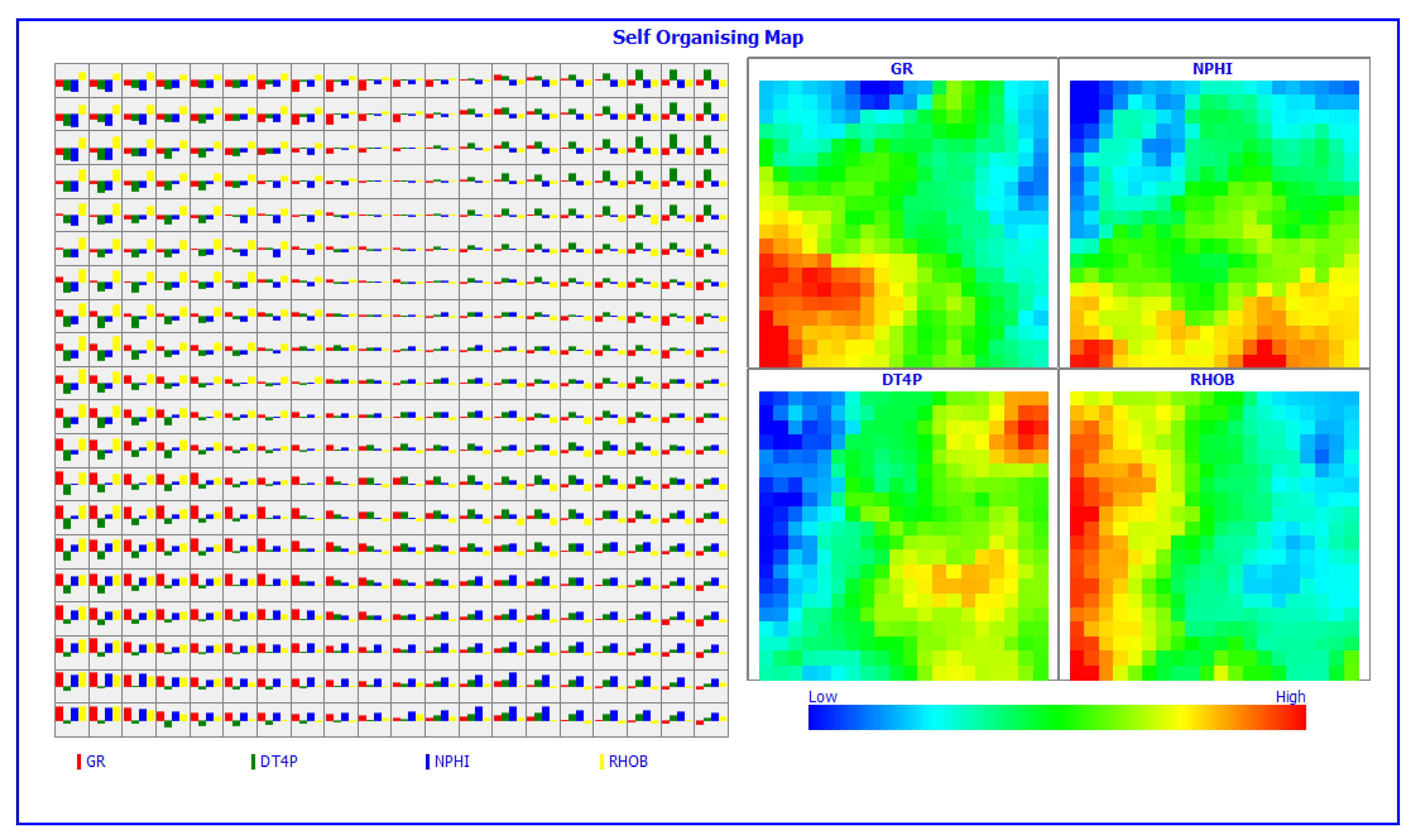
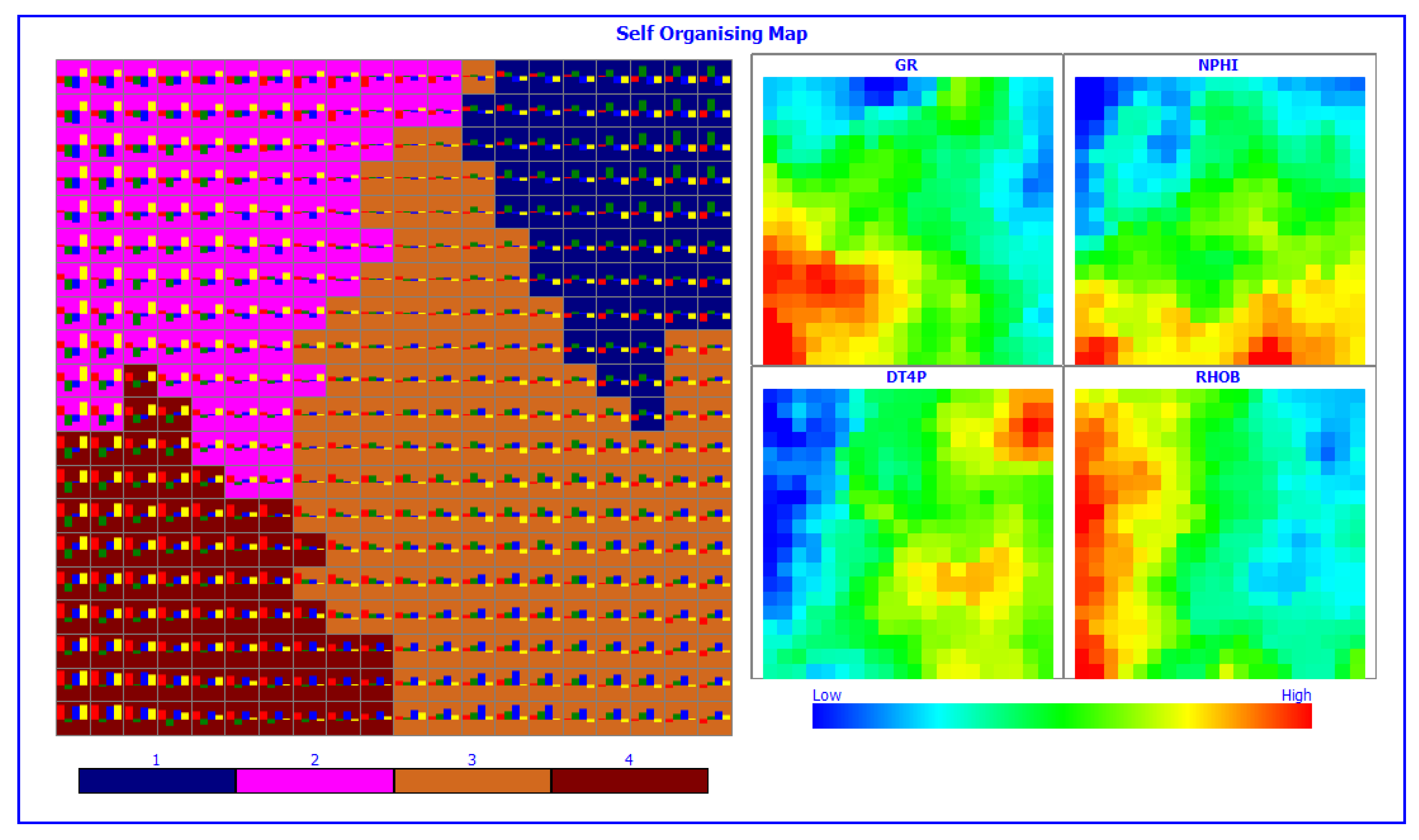
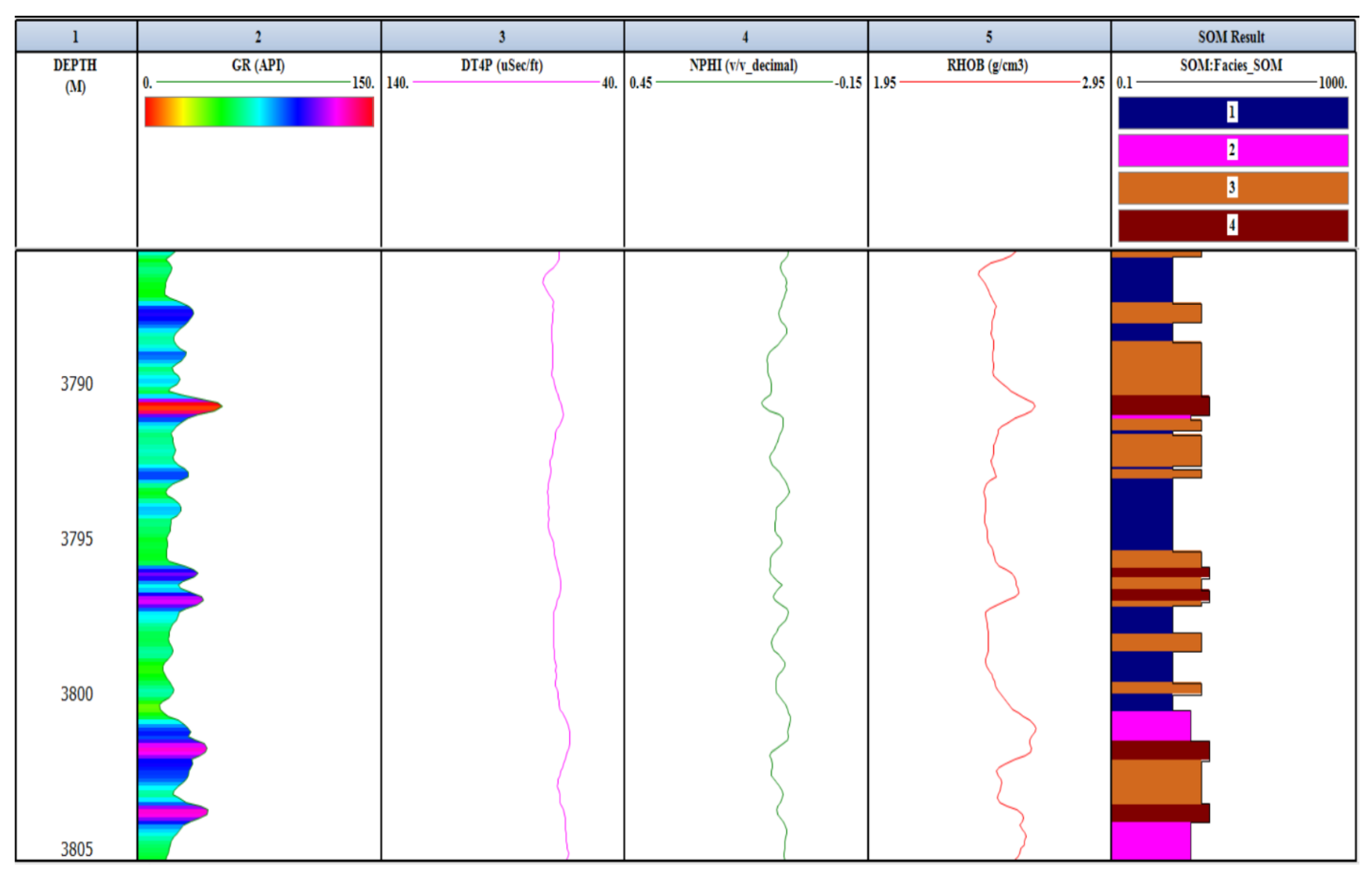
3.1. Self-Organizing Feature Map (SOFM) Approach for Lithofacies Identification

A self-organizing feature map (SOFM) was used to determine the accuracy of lithofacies. The findings of the SOFM model reveal four distinct lithofacies: Gamma Ray (GR), Neutron (NPHI), Sonic (DT4P), and Density (RHOB). The low and high scale represents that the relevant color code facies type is shown as a horizontal distribution to determine the lithological characteristics (Figure 4 and Figure 5). Vertical distribution features to determine the lithological characteristics of the interpreted well-3 are shown in Figure 6 and represent the calibration phase, in which we can clearly identify the vertical facies variation. These two figures cannot be combined because the (Figure 4) is the training phase, where is the (Figure 5) indicates the calibration phase, in which we can easily identify the horizontally facies variation. The found facies’ sedimentological elements vary little between reservoir intervals. The remaining facies “2” and “3” show a silty clay component, whereas facies “1” reveals pure sandstone. This approach also predicts the volume and hydrocarbon potential fluctuation of lithofacies. Sandstone with a small proportion of clay has moderate and low gas-bearing lithofacies, whereas sandstone with a small proportion of clay has moderate and low lithofacies. Lithology interpretation has been optimized as a result of the constant performance of the SOFM framework.

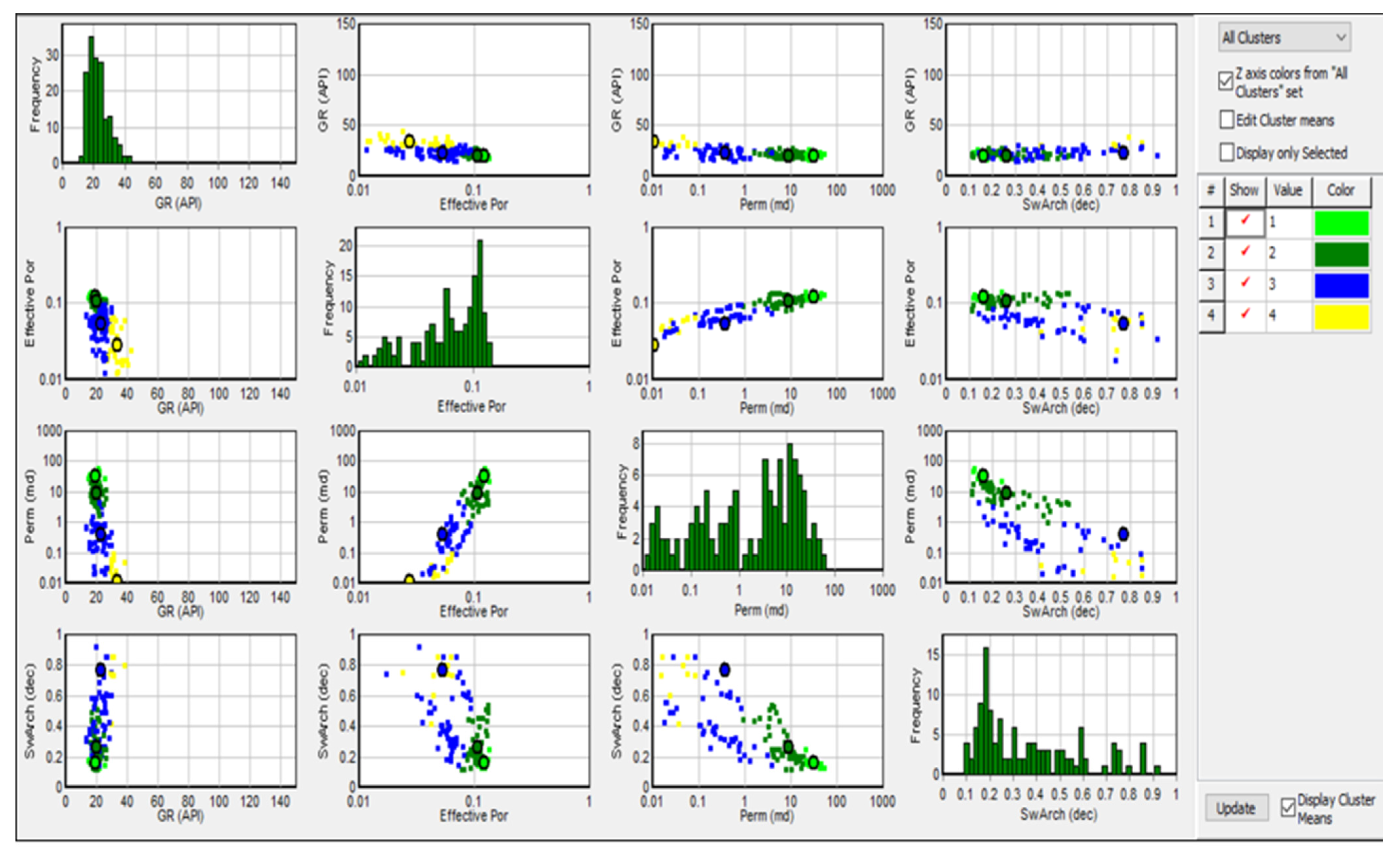
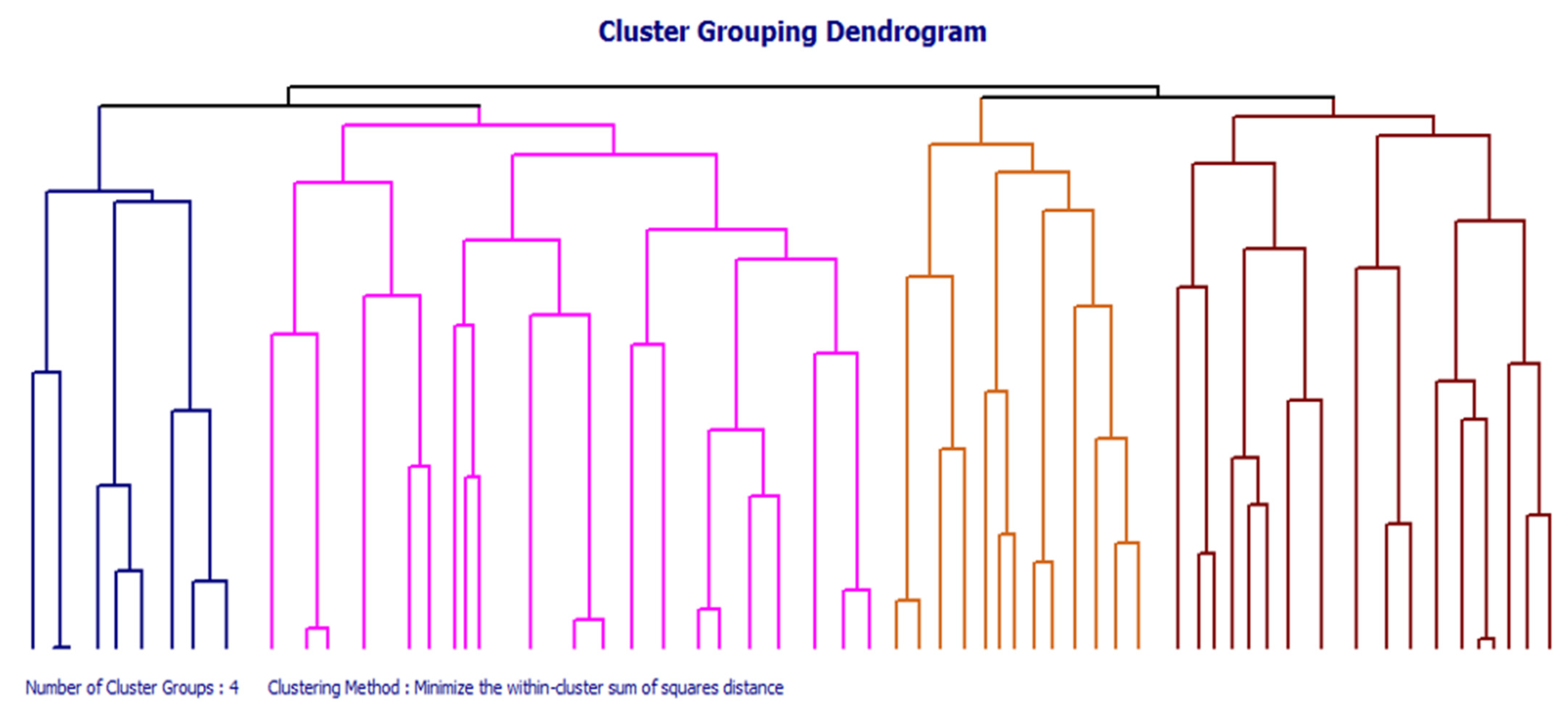
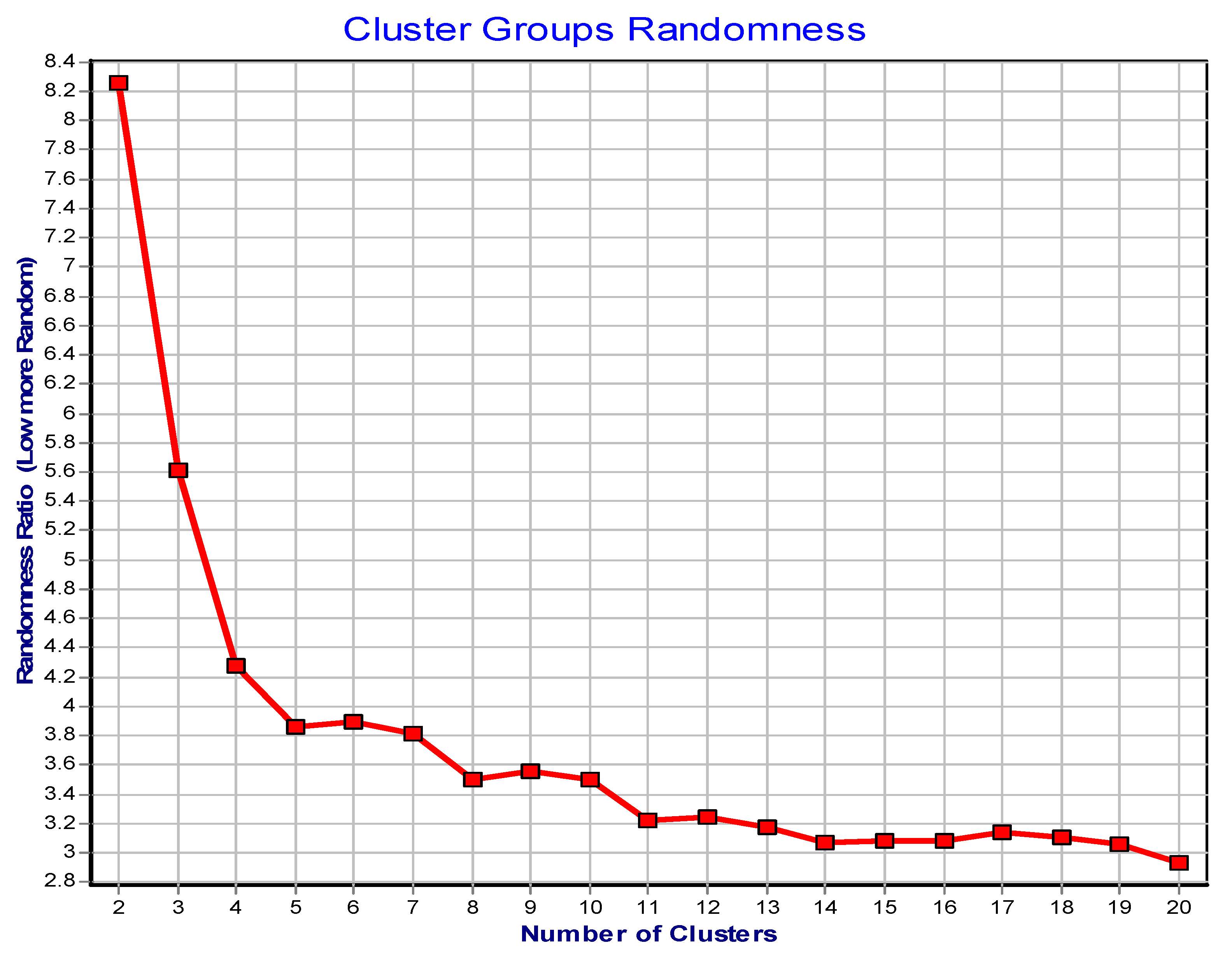
3.2. Cluster Analysis for Lithofacies Identification

The current study uses a cluster analysis technique to evaluate the efficacy of reservoir rock typing (RRT) of the identified sand masses. Cluster analysis is a multivariate strategy that seeks to divide a sample of subjects with a specific variable evaluated into a different number of groups, with like subjects grouped. An electrofacies is a unique set of log answers that characterizes the rock’s physical characteristics and fluids in the volume under investigation by logging tools. The rock types reflect reservoir bodies with a distinct relationship between effective porosity, deliverability, the potential for oil and gas storage, and the quantity of specific water saturation. It gives a good idea of how much oil is in the reservoir and how much is being recovered. The results of the cluster analysis show that the current study looked at rock intervals classified into four log facies. Each facies are described using the mean values of input log curves, and the “cluster means” findings for each well are shown in (Table 1). The results of the cluster assessment suggest that log facies 1 and 2 in the Cretaceous reservoir are the most interesting zones for the research area. Figure 7 shows the cluster analysis among the input data curves obtained using k-means clustering for facies groups, as well as the reservoir rock type properties of these log facies (Table 2).

3.3. Hierarchical and Non-Hierarchical

After calculating the distance between objects in the dataset, connecting distance data can be used to identify how objects in the dataset should be grouped into clusters. The objects with the shortest distance between them were joined together to form new clusters. These newly generated clusters link to one other and to add items to form larger clusters, eventually linking all of the objects in the original dataset in a hierarchical tree. In general, “minimum distance between all things in clusters” produces long, thin clusters, whereas “maximum distance between all objects in clusters” produces larger spherical clusters. The “minimize the within-cluster sum of squares distance” and “average distance between all objects in clusters” are likely to produce clusters that are comparable to those created with “average distance between all objects in clusters.” The clusters (electro-facies) were then constructed based on the data cluster tree or dendrogram (Figure 7). A dendrogram is a hierarchical tree with many U-shaped lines connecting things. The distance between two objects being connected is represented by the height of each U. Two objects with the shortest distance connect in the cluster tree to form a new, larger cluster. This sequence would repeat itself until just one cluster remained. For the dataset from all available wells, the procedure described above was used. As seen in Figure 8 of the dendrogram, the default approach “minimize the within-cluster sum of squares distance” produces good results for splitting the distinct log lithologies into different clusters. Stopping the grouping at a specific cutoff level makes it simple to divide the clusters into a defined number of groups. It is feasible to examine the groupings to determine whether adding another cluster adds more information or merely adds noise at which level. This information can be found in the “Cluster Randomness Plot.” The “Cluster Randomness Plot” that determines the perceived randomness of the data for each cluster group is shown in (Figure 9). The greater the score, the less random the clusters are, indicating that the data are more structured. The average number of depth levels per cluster, for example, the average thickness of a cluster layer, is used to determine unpredictability. This is carried out on the original log data. The theoretical average thickness is then determined, assuming that the clusters are assigned at each depth level at random. The ratio of the two is randomness. A value of 1 would be completely random, whereas higher values would be less so.
average thickness = number of depth levels/number of cluster layers
random   thickness = p i ( 1 p i )
where p i is the proportion of depth levels assigned to the i t h cluster.
Randomness index = average thickness = random thickness. The plot is interpreted by picking the number of least random clusters (highest peaks).

4. Discussion

The Zamzama Gas field in Pakistan was investigated using unsupervised learning and cluster analysis to categorize lithofacies and identify rock types. As both classifiers, hierarchical and non-hierarchical and SOFM produced more trustworthy results in lithofacies classification and rock type identification. These classifiers were able to accurately predict shaly sandstone and precision sandstone. However, when compared to other facies, the PR-area-under-curve score for shale was below average, indicating machine learning misclassification in predicting one facies to other facies despite the usually good accuracy. In comparison to the other facies, the existence of a mixture of shaly sand and sandstone has similar rock physical properties. Sandstone and shaly sandstone can be accurately categorized using the results of log-facies classification. On the other hand, shale distribution has been inconsistent. Furthermore, despite differences in rock physical properties between the different depths regions due to different rates of compaction and diagenetic processes, the machine learning model was able to properly predict lithofacies and rock type in both sections [27]. Due to the post-depositional processes that each formation underwent, the sensitivity of such a result may vary at deeper intervals, but despite this, the machine learning model has an overall high result and has effectively supported the geological investigation in a much shorter period [29,32]. The main contributions of this work were a simple approach for lithofacies classification and rock type identification in the Zamzama Gas field in Pakistan using SOM and cluster analysis, as well as hierarchical and non-hierarchical approaches, evaluation of each multiclass of unsupervised learning methods, high accuracy results despite some misclassification, log-facies classification analysis, and rock physics analysis based on unsupervised learning [33,34]. Most importantly, this study has demonstrated that the effectiveness of hierarchical and non-hierarchical SOFM can be evaluated from both a machine learning and geological perspective [29,35,36].

5. Conclusions

We have systematized the fundamental background of the SOM in this work. The U-matrix can also be used to view it, and BMUs can be seen directly. In addition, certain new changes have been made, such as normalization to standardize the input data and eliminating the scale value gap between curves. These contribute to a more accurate and realistic outcome. We also offered certain mathematical calculations, such as SOM, to help illustrate the process. Furthermore, attributes of the facies log are shown, such as the shape, measurement, and depth values. The input of the clustering process is also detailed in terms of SOM building. Based on log data, cluster analysis is a straightforward approach for determining the rock type for a reservoir. As illustrated in the roundness figure, cluster analysis of log data for wells that penetrated the reservoir were classified into four groups. Based on the cluster analysis, four facies have been identified; the findings of each facies are shown in (Table 1) and the behavior of each facies indicated in (Table 2). The results of these facies are shown in (Table 1) and (Table 2). Gamma Ray (GR), Effective Porosity(eff), Permeability (Perm) and Water Saturation (Sw) are used to generate these results. The Facies-01 zone in the reservoir for the Zamzama gas field is the most productive in the reservoir, as shown by plotting rock type in the continuous form in the well.

Author Contributions

M.H. and M.A. conceived this study. S.L. supervised this project. N.A. and A.A. undertook the responsibility of arranging the data for this project. M.H. and U.A. wrote the manuscript. W.H., A.A. and S.L. reviewed the manuscript and provided the necessary funding. All authors have read and agreed to the published version of the manuscript.

Funding

This research was supported by the National Natural Science Foundation of China (Grant Nos. 41874122 and 42122030).

Acknowledgments

The authors would like to thank the Directorate General of Petroleum Concessions (DGPC), Pakistan, for the release of well data. I am grateful to my supervisor for providing the necessary data, guidance, support, software, and technical help to accomplish this research. I am also thankful for my lab mates at the China University of Geosciences.

Conflicts of Interest

The authors declare no conflict of interest.

Nomenclature

SOMSelf-Organizing Map
SOFMSelf-Organizing Feature Map
PCAPrincipal Component Analysis
LGFLower Goru Formation
UGFUpper Goru Formation
BMUBest Matching Unit

References

  1. Ashraf, U.; Zhang, H.; Anees, A.; Mangi, H.N.; Ali, M.; Zhang, X.; Imraz, M.; Abbasi, S.S.; Abbas, A.; Ullah, Z. A Core Logging, Machine Learning and Geostatistical Modeling Interactive Approach for Subsurface Imaging of Lenticular Geobodies in a Clastic Depositional System, SE Pakistan. Nat. Resour. Res. 2021, 30, 2807–2830. [Google Scholar] [CrossRef]
  2. Ali, M.; Jiang, R.; Huolin, M.; Pan, H.; Abbas, K.; Ashraf, U.; Ullah, J. Machine Learning-A Novel Approach of Well Logs Similarity Based on Synchronization Measures to Predict Shear Sonic Logs. J. Pet. Sci. Eng. 2021, 203, 108602. [Google Scholar] [CrossRef]
  3. Bressan, T.S.; Kehl de Souza, M.; Girelli, T.J.; Junior, F.C. Evaluation of Machine Learning Methods for Lithology Classification Using Geophysical Data. Comput. Geosci. 2020, 139, 104475. [Google Scholar] [CrossRef]
  4. Ashraf, U.; Zhang, H.; Anees, A.; Mangi, H.N.; Ali, M.; Ullah, Z.; Zhang, X. Application of Unconventional Seismic Attributes and Unsupervised Machine Learning for the Identification of Fault and Fracture Network. Appl. Sci. 2020, 10, 3864. [Google Scholar] [CrossRef]
  5. Safaei-Farouji, M.; Vo Thanh, H.; Sheini Dashtgoli, D.; Yasin, Q.; Radwan, A.E.; Ashraf, U.; Lee, K.K. Application of Robust Intelligent Schemes for Accurate Modelling Interfacial Tension of CO2 Brine Systems: Implications for Structural CO2 Trapping. Fuel 2022, 319, 123821. [Google Scholar] [CrossRef]
  6. Vo-Thanh, H.; Amar, M.N.; Lee, K.K. Robust Machine Learning Models of Carbon Dioxide Trapping Indexes at Geological Storage Sites. Fuel 2022, 316, 123391. [Google Scholar] [CrossRef]
  7. Vo Thanh, H.; Lee, K.K. Application of Machine Learning to Predict CO2 Trapping Performance in Deep Saline Aquifers. Energy 2022, 239, 122457. [Google Scholar] [CrossRef]
  8. Thanh, H.V.; Van Binh, D.; Kantoush, S.A.; Nourani, V.; Saber, M.; Lee, K.; Sumi, T.; Sciences, E.; Korea, S.; Resources, W.; et al. Reconstructing Daily Discharge in a Megadelta Using Machine Learning Techniques. Water Resour. Res. 2022, 58. [Google Scholar] [CrossRef]
  9. Klose, C.D. Self-Organizing Maps for Geoscientific Data Analysis: Geological Interpretation of Multidimensional Geophysical Data. Comput. Geosci. 2006, 10, 265–277. [Google Scholar] [CrossRef]
  10. Al-Baldawi, B.A. Applying the Cluster Analysis Technique in Logfacies Determination for Mishrif Formation, Amara Oil Field, South Eastern Iraq. Arab. J. Geosci. 2015, 8, 3767–3776. [Google Scholar] [CrossRef]
  11. Nguyen, T.T.; Kawamura, A.; Tong, T.N.; Nakagawa, N.; Amaguchi, H.; Gilbuena, R. Clustering Spatio-Seasonal Hydrogeochemical Data Using Self-Organizing Maps for Groundwater Quality Assessment in the Red River Delta, Vietnam. J. Hydrol. 2015, 522, 661–673. [Google Scholar] [CrossRef]
  12. Sfidari, E.; Kadkhodaie-Ilkhchi, A.; Rahimpour-Bbonab, H.; Soltani, B. A Hybrid Approach for Litho-Facies Characterization in the Framework of Sequence Stratigraphy: A Case Study from the South Pars Gas Field, the Persian Gulf Basin. J. Pet. Sci. Eng. 2014, 121, 87–102. [Google Scholar] [CrossRef]
  13. Garća, H.L.; González, I.M. Self-Organizing Map and Clustering for Wastewater Treatment Monitoring. Eng. Appl. Artif. Intell. 2004, 17, 215–225. [Google Scholar] [CrossRef]
  14. Unglert, K.; Radić, V.; Jellinek, A.M. Principal Component Analysis vs. Self-Organizing Maps Combined with Hierarchical Clustering for Pattern Recognition in Volcano Seismic Spectra. J. Volcanol. Geotherm. Res. 2016, 320, 58–74. [Google Scholar] [CrossRef]
  15. Hsieh, B.Z.; Lewis, C.; Lin, Z.S. Lithology Identification of Aquifers from Geophysical Well Logs and Fuzzy Logic Analysis: Shui-Lin Area, Taiwan. Comput. Geosci. 2005, 31, 263–275. [Google Scholar] [CrossRef]
  16. Al-Anazi, A.; Gates, I.D. A Support Vector Machine Algorithm to Classify Lithofacies and Model Permeability in Heterogeneous Reservoirs. Eng. Geol. 2010, 114, 267–277. [Google Scholar] [CrossRef]
  17. Imamverdiyev, Y.; Sukhostat, L. Lithological Facies Classification Using Deep Convolutional Neural Network. J. Pet. Sci. Eng. 2019, 174, 216–228. [Google Scholar] [CrossRef]
  18. Male, F.; Duncan, I.J. Lessons for Machine Learning from the Analysis of Porosity-Permeability Transforms for Carbonate Reservoirs. J. Pet. Sci. Eng. 2020, 187, 106825. [Google Scholar] [CrossRef]
  19. Deng, Z.; Zhu, X.; Cheng, D.; Zong, M.; Zhang, S. Efficient KNN Classification Algorithm for Big Data. Neurocomputing 2016, 195, 143–148. [Google Scholar] [CrossRef]
  20. Vo Thanh, H.; Sugai, Y.; Nguele, R.; Sasaki, K. A New Petrophysical Modeling Workflow for Fractured Granite Basement Reservoir in Cuu Long Basin, Offshore Vietnam. In Proceedings of the 81st EAGE Conference and Exhibition, London, UK, 3–6 June 2019; European Association of Geoscientists & Engineers: London, UK, 2019; pp. 1–5. [Google Scholar]
  21. Anees, A.; Zhang, H.; Ashraf, U.; Wang, R.; Liu, K.; Abbas, A.; Ullah, Z.; Zhang, X.; Duan, L.; Liu, F.; et al. Sedimentary Facies Controls for Reservoir Quality Prediction of Lower Shihezi Member-1 of the Hangjinqi Area, Ordos Basin. Minerals 2022, 12, 126. [Google Scholar] [CrossRef]
  22. Anees, A.; Zhang, H.; Ashraf, U.; Wang, R.; Liu, K.; Mangi, H.N.; Jiang, R.; Zhang, X.; Liu, Q.; Tan, S.; et al. Identification of Favorable Zones of Gas Accumulation via Fault Distribution and Sedimentary Facies: Insights from Hangjinqi Area, Northern Ordos Basin. Front. Earth Sci. 2022, 9, 822670. [Google Scholar] [CrossRef]
  23. Jiang, R.; Zhao, L.; Xu, A.; Ashraf, U.; Yin, J.; Song, H.; Su, N.; Du, B.; Anees, A. Sweet Spots Prediction through Fracture Genesis Using Multi-Scale Geological and Geophysical Data in the Karst Reservoirs of Cambrian Longwangmiao Carbonate Formation, Moxi-Gaoshiti Area in Sichuan Basin, South China. J. Pet. Explor. Prod. Technol. 2021, 12, 1313–1328. [Google Scholar] [CrossRef]
  24. Ullah, J.; Luo, M.; Ashraf, U.; Pan, H.; Anees, A.; Li, D.; Ali, M.; Ali, J. Evaluation of the Geothermal Parameters to Decipher the Thermal Structure of the Upper Crust of the Longmenshan Fault Zone Derived from Borehole Data. Geothermics 2022, 98, 102268. [Google Scholar] [CrossRef]
  25. Abbas, A.; Zhu, H.; Anees, A.; Ashraf, U.; Akhtar, N. Integrated Seismic Interpretation, 2d Modeling along with Petrophysical and Seismic Atribute Analysis to Decipher the Hydrocarbon Potential of Missakeswal Area. Pakistan. J. Geol. Geophys. 2019, 7, 1–12. [Google Scholar]
  26. Anees, A.; Zhong, S.W.; Ashraf, U.; Abbas, A. Development of a Computer Program for Zoeppritz Energy Partition Equations and Their Various Approximations to Affirm Presence of Hydrocarbon in Missakeswal Area. Geosciences 2017, 7, 55–67. [Google Scholar] [CrossRef]
  27. Shehata, A.A.; Osman, O.A.; Nabawy, B.S. Journal of Natural Gas Science and Engineering Neural Network Application to Petrophysical and Lithofacies Analysis Based on Multi-Scale Data: An Integrated Study Using Conventional Well Log, Core and Borehole Image Data. J. Nat. Gas Sci. Eng. 2021, 93, 104015. [Google Scholar] [CrossRef]
  28. Wang, G.; Carr, T.R.; Ju, Y.; Li, C. Identifying Organic-Rich Marcellus Shale Lithofacies by Support Vector Machine Classifier in the Appalachian Basin. Comput. Geosci. 2014, 64, 52–60. [Google Scholar] [CrossRef]
  29. Freund, Y. Boosting a Weak Learning Algorithm by Majority. Inf. Comput. 1995, 121, 256–285. [Google Scholar] [CrossRef]
  30. Al Kattan, W.; Jawad, S.N.A.L.; Jomaah, H.A. Cluster Analysis Approach to Identify Rock Type in Tertiary Reservoir of Khabaz Oil Field Case Study. Iraqi J. Chem. Pet. Eng. 2018, 19, 9–13. [Google Scholar]
  31. Mandal, P.P.; Rezaee, R. Facies Classification with Different Machine Learning Algorithm–An Efficient Artificial Intelligence Technique for Improved Classification. ASEG Ext. Abstr. 2019, 2019, 1–6. [Google Scholar] [CrossRef] [Green Version]
  32. Shahid, A.R.; Khan, S.; Yan, H. Human Expression Recognition Using Facial Shape Based Fourier Descriptors Fusion. In Proceedings of the Twelfth International Conference on Machine Vision (ICMV 2019), Amsterdam, The Netherlands, 16–18 November 2019; Volume 11433, p. 48. [Google Scholar] [CrossRef]
  33. Qureshi, M.A.; Ghazi, S.; Riaz, M.; Ahmad, S. Geo-Seismic Model for Petroleum Plays an Assessment of the Zamzama Area, Southern Indus Basin, Pakistan. J. Pet. Explor. Prod. Technol. 2020, 1–12. [Google Scholar] [CrossRef]
  34. Ahmed Abbasi, S.; Asim, S.; Solangi, S.H.; Khan, F. Study of Fault Configuration Related Mysteries through Multi Seismic Attribute Analysis Technique in Zamzama Gas Field Area, Southern Indus Basin, Pakistan. Geod. Geodyn. 2016, 7, 132–142. [Google Scholar] [CrossRef] [Green Version]
  35. Mangi, H.N.; Chi, R.; DeTian, Y.; Sindhu, L.; Lijin; He, D.; Ashraf, U.; Fu, H.; Zixuan, L.; Zhou, W.; et al. The Ungrind and Grinded Effects on the Pore Geometry and Adsorption Mechanism of the Coal Particles. J. Nat. Gas Sci. Eng. 2022, 100, 104463. [Google Scholar] [CrossRef]
  36. Mangi, H.N.; Detian, Y.; Hameed, N.; Ashraf, U.; Rajper, R.H. Pore Structure Characteristics and Fractal Dimension Analysis of Low Rank Coal in the Lower Indus Basin, SE Pakistan. J. Nat. Gas Sci. Eng. 2020, 77, 103231. [Google Scholar] [CrossRef]
  37. Ehsan, M.; Gu, H.; Akhtar, M.M.; Abbasi, S.S.; Ehsan, U. A Geological Study of Reservoir Formations and Exploratory Well Depths Statistical Analysis in Sindh Province, Southern Lower Indus Basin, Pakistan. Kuwait J. Sci. 2018, 45, 84–93. [Google Scholar]
  38. Foredeep, K. A radical seismic interpretation re-think resolves the structural complexities of the zamzama field, kirthar foredeep, pakistan. In Proceedings of the SPE Annual Technical Conference, Islamabad, Pakistan, 10–12 December 2018; pp. 1–17. [Google Scholar]
  39. Asim, S.; Qureshi, S.N.; Asif, S.K.; Abbasi, S.A.; Solangi, S.; Mirza, M.Q. Structural and Stratigraphical Correlation of Seismic Profiles between Drigri Anticline and Bahawalpur High in Central Indus Basin of Pakistan. Int. J. Geosci. 2014, 5, 1231–1240. [Google Scholar] [CrossRef] [Green Version]
  40. Sirimangkhala, K.; Pimpunchat, B.; Amornsamankul, S.; Triampo, W. Modelling Greenhouse Gas Generation for Landfill. Int. J. Simul. Syst. Sci. Technol. 2018, 19, 16.1–16.7. [Google Scholar] [CrossRef]
  41. Ashraf, U.; Zhu, P.; Yasin, Q.; Anees, A.; Imraz, M.; Mangi, H.N.; Shakeel, S. Classification of Reservoir Facies Using Well Log and 3D Seismic Attributes for Prospect Evaluation and Field Development: A Case Study of Sawan Gas Field, Pakistan. J. Pet. Sci. Eng. 2019, 175, 338–351. [Google Scholar] [CrossRef]
  42. Ashraf, U.; Zhang, H.; Anees, A.; Ali, M.; Zhang, X.; Shakeel Abbasi, S.; Nasir Mangi, H. Controls on Reservoir Heterogeneity of a Shallow-Marine Reservoir in Sawan Gas Field, SE Pakistan: Implications for Reservoir Quality Prediction Using Acoustic Impedance Inversion. Water 2020, 12, 2972. [Google Scholar] [CrossRef]
  43. Ali, M.; Ma, H.; Pan, H.; Ashraf, U.; Jiang, R. Building a Rock Physics Model for the Formation Evaluation of the Lower Goru Sand Reservoir of the Southern Indus Basin in Pakistan. J. Pet. Sci. Eng. 2020, 194, 107461. [Google Scholar] [CrossRef]
  44. Dar, Q.U.Z.; Pu, R.; Baiyegunhi, C.; Shabeer, G.; Ali, R.I.; Ashraf, U.; Sajid, Z.; Mehmood, M. The Impact of Diagenesis on the Reservoir Quality of the Early Cretaceous Lower Goru Sandstones in the Lower Indus Basin, Pakistan. J. Pet. Explor. Prod. Technol. 2021, 12, 1437–1452. [Google Scholar] [CrossRef]
  45. Ali, N.; Chen, J.; Fu, X.; Hussain, W.; Ali, M.; Hussain, M.; Anees, A.; Rashid, M.; Thanh, H.V. Prediction of Cretaceous Reservoir Zone through Petrophysical Modeling: Insights from Kadanwari Gas Field, Middle Indus Basin. Geosystems Geoenviron. 2022, 1, 100058. [Google Scholar] [CrossRef]
  46. Chon, T.S. Self-Organizing Maps Applied to Ecological Sciences. Ecol. Inform. 2011, 6, 50–61. [Google Scholar] [CrossRef]
Figure 1. (a) Satellite map showing the locations of the major oil and gas filed within the Middle and Southern Indus Basin. Zamzama gas field is present in the middle towards the eastern side of the map. (b) Regional tectonic map of Pakistan, showing the major basins and tectonic regions.
Energies 15 04501 g001aEnergies 15 04501 g001b
Figure 2. Generalized lithostratigraphy of the Lower Indus Basin [34].
Energies 15 04501 g002
Figure 3. Diagram of Cluster Z.
Energies 15 04501 g003
Figure 4. Self-organising map before calibration.
Energies 15 04501 g004
Figure 5. Component SOM model planes for the four input parameters after calibration.
Energies 15 04501 g005
Figure 6. SOM vertical distribution model showing the interpreted lithofacies for the four input parameters after calibration.
Energies 15 04501 g006
Figure 7. The final graphical result of clustering analysis.
Energies 15 04501 g007
Figure 8. Cluster grouping dendrogram of the Zamzama Gas Field.
Energies 15 04501 g008
Figure 9. Cluster groups randomness of Zamzama Gas Field.
Energies 15 04501 g009
Table 1. The results of “cluster means” plus other statistics of user data for each cluster.
K-Mean Cluster Results
GReffPermSw
FaciesPointsRock TypingMeanMeanMeanMean
113Excellent-quality rock type19.440.1232.490.16
250Good-quality rock type20.320.108.940.26
362Moderate-quality rock type22.590.050.370.77
435Poor-quality rock type33.340.020.0134.69
Table 2. The properties for groups of Facies.
S. NoRock TypingGReffPermSw
Facies-01Excellent-quality rock typeVery lowGood to excellentGood to excellentVery low
Facies-02Good-quality rock typelowGood Goodlow
Facies-03Moderate-quality rock typeMediumFair to GoodFair to GoodMedium
Facies-04Poor-quality rock typeHighLowLowVery high
Publisher’s Note: MDPI stays neutral with regard to jurisdictional claims in published maps and institutional affiliations.

