Optimizing Low-Carbon Pathway of China’s Power Supply Structure Using Model Predictive Control

Abstract

With the increasing severity of climate change, the power industry, as one of the main sources of carbon emissions, is playing an extremely important role in the process of low-carbon energy transformation. The purpose of this paper is to try to find a general method to solve the optimal path for the low-carbon evolution of the power supply structure so as to meet the challenges faced by the low-carbon transformation of the power industry in the future. This paper first uses the capacity coefficient index (CCI) to represent the power generation ability of different technologies and proposes a forecasting method for the CCI of renewable energy generation. In this paper, a two-layer optimization model considering multiple constraints is established and solved using the MPC method. The results show that China’s installed capacity of renewable power could account for more than 50% in 2030, while the carbon emissions will decrease after reaching a peak in 2023. On the premise of ensuring sufficient reserve adjustment capacity of thermal power units, increasing the proportion of renewable energy generation is an important way to realize emission reduction in the power industry.

1. Introduction

In recent years, climate change has intensified, and the negative impacts of a rising global mean temperature as well as frequent extreme weather on the development of economic society have become increasingly prominent. In addition to directly causing the global average temperature to rise, climate change will also indirectly have an important impact on global agriculture, animal husbandry [1,2,3], the water resources cycle [4,5], and natural disasters [6]. Some scholars have attempted to assess the negative impacts of climate change from the perspective of the driving factors of climate change risks and provide a scientific basis for policy formulation [7], but how humans can adapt to the increasingly severe climate change situation is still a global problem that needs to be solved urgently. Apparently, the root cause of climate change is the increase in annual greenhouse gas emissions, of which carbon dioxide emissions are the most significant. The signing of the Paris Agreement in 2016 was a milestone in the course of global climate governance [8]. It put forward long-term planning goals for future climate change and clarified the emission reduction responsibilities that all countries in the world should undertake. Although it may be difficult to achieve the ideal temperature control targets according to the current emission reduction commitments made by countries, it is still of great significance to the climate governance process [9]. As the largest developing country in the world, China ranks first in carbon dioxide emissions. In response to the call for emission reduction, China has put forward the ambitious goal of achieving a carbon peak by 2030 and carbon neutrality by 2060, i.e., the “double carbon” goal [10]. Carbon emission constraints have become an important factor restricting the development of China’s future energy industry.

In order to achieve the “double carbon” goal, all industries have accelerated the energy transition from fossil to non-fossil energy. The main cause of carbon dioxide emissions is the combustion of fossil fuels in industrial production, with energy-intensive industries, such as electricity, transportation, and construction, producing the vast majority of carbon emissions. As an important part of the modern energy industry, the low-carbon transformation of the power industry is playing an important role in the transformation of the entire energy industry. There is no doubt that the power generation side produces the vast majority of carbon emissions in the power industry. Coal-fired plants consume a large amount of coal resources every year to meet the huge electricity demand while producing high carbon emissions [11]. Shuai, Y. et al. analyzed the main technologies for improving the operating efficiency and reducing the carbon emissions of coal-fired units, and looked forward to their development prospects [12]. In fact, supercritical and ultra-supercritical units improve the energy utilization efficiency, but cannot fundamentally solve the problem of high emissions from coal-fired units. Some studies have attempted to reduce carbon emissions by adding carbon capture and storage (CCS) devices to coal-fired power plants [13,14], but CCS technology is still unclear and has not been put into commercial application [15]. This means that thermal power units may be obsolete in the future if there is no major technological breakthrough. Other types of units, while not producing carbon emissions, may incur higher external costs during construction or operation. Unreasonable hydropower construction not only fails to make full use of hydro resources, but also causes irreversible damage to human conditions and the ecological environment [16,17]. In addition, the driving force for nuclear power plant expansion depends on the current control level over nuclear energy, and especially after the Fukushima nuclear power plant accident, the public has had a psychological resistance to nuclear power technology [18]. Although the nuclear power generation technology has returned to the public eye due to the increasing pressure of emission reduction in recent years, it has to be admitted that the development of nuclear power requires a higher technical level and management ability. Power generation by renewable energy, such as wind power and solar energy, has grown rapidly in recent years, and there is still a lot of room for development.

In view of the huge pressure of emission reduction, more and more scholars and research institutions are conducting research on the low-carbon transformation path of the energy industry. Finding the optimal path for the low-carbon evolution of the power structure under multiple constraints considering the characteristics of different power generation technologies has become a research hotspot in the academic community. The International Energy Agency (IEA) predicted the future power supply structure of China by setting different emission reduction scenarios, and proved that the realization of the “double carbon” goal relies on the vigorous development of renewable energy [19]. Literature [20] has explored the impact of China’s renewable energy policy on the power supply structure and indicated that the low-carbon transformation of the power industry is inseparable from the strong support of the government. Reference [21] applied the scenario analysis method to forecast the power structure and carbon emissions under different scenarios in the future, and proved that a strict emission reduction policy is a strong guarantee for the realization of emission reduction in the power industry. Shen, W. et al. analyzed the decommissioning problem of old coal-fired power plants and calculated the carbon emissions on the demand side using the carbon emission flow model. An installed capacity expansion strategy was proposed considering aging, decommissioning, and carbon emissions [22]. Reference [23] established a multi-objective power structure optimization model with minimum system cost and minimum carbon emissions, and then solved the optimal path of future power structure evolution. In 2035, the carbon emissions from the power industry will be below 4 billion tons, according to the results of simulation. Li, Z. et al. proposed a joint optimization model for the long-term planning and short-term operation of the power system considering carbon constraints, which determined the changing trends of various power generation technologies over time. The installed capacity of non-fossil energy will account for more than 93% in 2050 under the 2 °C scenario [24]. On the basis of the carbon budget assessment, Shu, Y. et al. built a path-planning-optimization model, including the power structure, power carbon emissions, and operating cost, then determined the low-carbon transformation path under different scenarios [25]. The results show that, if the carbon emissions of the power industry are negative in 2060, the installed capacity and power generation of non-fossil energy should account for more than 92% and 94%, respectively. The most representative “bottom-up” energy system models are the Technology Market Allocation Model (MARKAL) and the Energy Flow Optimization Model (EFOM), which have a wide range of applications in the energy field. Reference [26] considered the differences in resources and technical conditions between different regions and introduced the comprehensive MARKAL-EFOM system (TIMES) model of China’s regional power sector to obtain the regional optimal power supply structure under each emission scenario. In addition, the Long-range Energy Alternatives Planning System (LEAP) model is also a powerful tool for carbon emissions analysis in the power industry. Mirjat, N.H. et al. used the LEAP tool to predict the electricity demand and emission-reduction potential of Pakistan’s power system under different economic levels and low-carbon technology scenarios, and then provided the recommendations devised from the study [27]. To analyze the impact of extreme weather conditions on the planning of the electrical power supply, Wang, B. et al. explained the main reason for power supply shortage and used the improved LEAP model to predict the thermal power generation and installed capacity under normal and extreme weather scenarios in 2025 and 2030, respectively [28]. The case studies show that, when extreme weather occurs frequently, fossil energy is still required to ensure power supply security, which means that the power industry will still have high emissions in the near future.

An important factor affecting power structure planning is the uncertainty of renewable energy. Renewable energy power outputs are vulnerable to external natural conditions, and a high proportion of grid-connected renewable energy brings high uncertainty to the system. Reference [29] introduced the current situation of wind power generation in China and analyzed the reasons for the mismatch between the installed capacity and power generation of wind power. Predicting the output of renewable energy, such as wind and solar energy, has always been the focus of academic research. Probabilistic forecasting methods and artificial intelligence methods have been widely used in wind power and photovoltaic output forecasting [30,31,32], which is becoming mature. Demand response (DR) is an important method to mobilize demand-side resources to adapt to uncertain factors, such as climate change. A reasonable control strategy will improve resource utilization efficiency and reduce operating costs. Reference [33] explored the impact of DR actions on the thermal comfort and electricity cost for residential houses. Combining electricity price fluctuations and weather information, a DR control strategy was proposed to ensure residents’ thermal comfort while reducing electricity costs. Reference [34] studied the impact of the DR actions of residential thermal storage systems on energy consumption and cost under cold conditions, and proposed a predictive control algorithm based on the trend of electricity price changes. The results showed that the DR action strategy based on this algorithm will reduce the annual delivered energy for the heating system by 12% and energy cost by 11%, which would not be related to building structure. Reference [35] quantified the energy-use behavior of residents and proposed an optimal DR dispatch strategy covering electric vehicles. With reasonable electricity price incentives, this strategy will play a role in improving the consumption rate of renewable energy. In addition to DR, the power system also needs to adopt some strategies to overcome the uncertainty of renewable energy. de Siqueira, L. et al. used the control strategy of the energy storage system to smooth the output of wind power, which has guiding significance for the regulation and operation of a power grid [36]. Fan, M. proposed a new optimal power generation scheduling algorithm that can help to reduce the bus voltage changes under the fluctuation of new energy power generation and improve the adaptability of the power system to short-term power changes [37]. Previous studies have shown that the current power supply structure combined with a corresponding control strategy can suppress the negative impacts of the volatility of renewable energy, to a certain extent. However, it is still necessary to ensure that the power system has sufficient-flexibility resources, which is also one of the factors that must be considered in the power structure planning of modern power systems.

Among the commonly used control models, model-predictive control (MPC) adjusts the control strategy in time according to the existing state and acts on the adjacent control time domain. The MPC method includes model prediction, control action, and feedback correction, and is widely used in various fields. Ye, L. et al. sorted out the research status of MPC in the field of wind power prediction as well as control and conducted an in-depth analysis of three types of commonly used MPC methods, expounding the advantages and disadvantages of MPC methods [38]. The method based on load frequency control using MPC proposed in reference [39], which is suitable for multi-regional power systems, uses multi-variable constraints to calculate the optimal control scheme and verifies the superiority of MPC compared with traditional control methods. Zheng, Y. et al. applied MPC to the optimal dispatching of wind farms with energy storage systems and performed optimal control based on short-term measurement data of wind speed in the rolling time domain to minimize energy loss [40]. Reference [41] designed an energy-management system based on MPC and successive linear programming. This new MPC method could effectively reduce the energy cost of the community. Case studies have shown that the application of this energy management system can reduce the community electricity energy cost by 5.4–7.7%. The DICE model proposed in [42] applies dynamic optimization to climate economics and uses MPC to optimize the development path of future savings rates and emission reduction rates, demonstrating the practicality of dynamic optimization in long-term planning work. The MPC has obvious advantages in the field of optimal control; however, most researchers use it for short-term scheduling optimization and fail to apply it to long-term planning of power supply structure.

It is worth noting that most of the existing research on power structure planning only regarded the impact of renewable energy generation uncertainty on power planning as an inequality constraint. An in-depth study of the annual power generation fluctuations of renewable energy units has not been carried out. At the same time, the current power planning is mostly based on scenario-based future power structure prediction, and it is difficult to adjust the optimization strategy for different states in different time periods. Few studies have regarded power structure planning as a dynamic programming problem. In order to fill the gap of research in this area, this paper proposes the concept of a capacity coefficient index (CCI) to describe the annual power generation ability of a certain generation technology and transforms the CCI of renewable energy generation into a probabilistic problem. On the basis of the above ideas, this paper establishes a two-layer optimization model and uses the MPC framework to solve the problem. Finally, the optimal evolution path of China’s power supply structure from 2020 to 2030 is obtained. The main innovations and contributions of this paper are as follows.

(1)

Establish the concept of CCI to describe the relationship between installed capacity and annual generation, put forward a statistical-based CCI simulation method for renewable energy units, and extend the method to annual power structure planning;

(2)

Establish a two-layer optimization structure, regard power structure planning as two stages of installed capacity optimization and power generation optimization, and solve the optimization problem in stages;

(3)

Apply the MPC framework to power supply structure planning, regard the problem as a dynamic programming problem, solve the optimization problem from the control perspective, adjust the control strategy of each rolling time domain according to different states, and finally obtain the optimal solution.

The structure of each part of this paper is as follows. Section 1 summarizes the research status. Section 2 introduces relevant concepts and methods. Section 3 establishes a mathematical model of the research problem and proposes a solution method. Section 4 uses the model established in this paper to carry out an example simulation. Section 5 discusses the results of the example and Section 6 draws the main conclusions.

2. Introduction of Related Concepts

2.1. CCI of the Generator

The high proportion of renewable energy generation is the main way for the power industry to achieve low-carbon transformation, and it is a prominent feature of the modern power system. With the continued expansion of renewable energy units, the resulting problems have become increasingly prominent. The most important one is the hidden danger of power supply security caused by the uncertainty of renewable energy. The power generation capacity of renewable energy units may not be reliable under certain extreme conditions, and this factor restricts the rapid withdrawal of fossil energy units. In order to express the power generation ability of renewable energy units, it is necessary to introduce the concept of CCI.

CCI is an indicator describing the annual power generation per unit of installed capacity of a certain generation technology, which is numerically equal to the ratio of the annual power generation to the installed capacity, as shown in Equation (1).

$$n_i=\frac{W_i}{G_i},$$

(1)

where $W_i$ represents the total annual power generation of power generation technology I, in kWh; $G_i$ is the annual installed capacity of power generation technology i, in kW; and $n_i$ is the CCI value corresponding to power generation technology i. From Equation (1), $n_i$ is in hours (h).

The CCI of each power generation technology varies greatly. The CCI of nuclear power is almost twice as large as that of ordinary hydropower, which means that nuclear power with less installed capacity can generate more electricity. Due to differences in operation mode, the CCI of each power generation technology varies over the years, but the fluctuation range is not large. While meeting the basic load, thermal power units generally need to undertake the task of peak shaving due to their excellent regulation performance. In many cases, it is impossible to generate electricity according to the initial set standard, especially for deep peak shaving units that have undergone flexibility transformation—their CCI will be far below the rated standard. Unlike thermal power units, due to the uncertainty of power generation by renewable energy units, CCI also has a certain degree of randomness. Even if the abandonment rate of renewable energy is reduced as much as possible according to the current scientific and technological means, CCI is relatively low and uncontrollable. Generally speaking, the CCI of a renewable energy unit reflects the mismatch between its installed capacity and total power generation—large installed capacity does not mean large power generation due to the low CCI. The non-controllability of renewable energy units is a factor that must be considered in annual power balance planning.

2.2. Forecast of CCI for Renewable Energy Units

The CCI of renewable energy is susceptible to natural environmental conditions and has a high degree of uncertainty. This paper assumes that the advanced regulation and operation technology of renewable energy generation is fully utilized, and its CCI is only relevant to natural conditions in this context. We believe that the annual power generation of a certain renewable energy unit in recent years has a similar law if the natural conditions are the same, which means that the CCI of a certain renewable energy technology can be predicted through historical data under the premise of considering some disturbances. These disturbances are mainly caused by natural factors, such as irregular fluctuations in renewable energy, and unnatural factors, such as changes in operating modes. In this paper, the CCI value of future renewable energy power generation is regarded as the superposition of the foreseeable amount and the random amount, which means that the CCI value of the next year is the result of the combined action of the empirical forecast value and random disturbance. The foreseeable amount and the random amount represent the general law and uncertainty of renewable energy output, respectively. The foreseeable quantities are estimated using the average of three-year CCI historical data, and the random quantities are generated using the statistical method proposed in Section 2.3. Equation (2) is the prediction formula of CCI.

$$\begin{array}{ll}n(j+1)& =\frac{1}{3}(n(j)+n(j-1)+n(j-2))+\epsilon \\ & =n_{predict}+\epsilon \end{array}$$

(2)

where j is the year relative to starting year in planning period and $n(j)$, $n(j-1)$, and $n(j-2)$ are the CCIs of the unit in the year j and the past two years; and $\epsilon$ is the disturbance term due to the randomness of natural factors and unnatural factors, which obeys the normal distribution of $N(\mu ,{\sigma }^2)$. Each value of the disturbance term $\epsilon$ corresponds to a random scenario, and $n(j+1)$ is the predicted value of CCI for the year j + 1 under this scenario. Due to the existence of uncertainty, assuming that the random item obeys the normal distribution, a series of random numbers are generated by statistical methods—each group of random numbers represents a certain path of the future evolvement of the random item $\epsilon$. By using the method proposed in Equation (2), with multiple scenarios of renewable energy obtained, the mathematical expectation of CCI under multiple scenarios is determined as the final prediction value of CCI in this paper, as shown in Equation (3).

$$n_p=E(n)=\frac{1}{L}{\displaystyle \sum _{l\in L}{n}_l},$$

(3)

where $n_i$ is the predicted value of CCI under scenario l, L is the total number of scenarios, E represents the mathematical expectation, and $n_p$ is the final predicted value.

2.3. Latin Hypercube Sampling

Latin hypercube sampling (LHS) is a type of stratified random sampling, which has a wide range of applications in probability statistics. This method first divides the sampling unit into different layers according to a certain characteristic or a certain rule, and then selects samples from different layers to ensure that the structure of the samples is relatively similar to the overall structure, thereby improving the accuracy of the estimation. In view of the advantages of the LHS method, some scholars have used this method to model randomness problems. Li, Q. et al. proposed an improved LHS method applied to the grid system with distributed generation, which improved the efficiency and accuracy of the probabilistic power flow algorithm [43]. Zhao, W. et al. proposed an LHS method suitable for random variables and demonstrated the superiority of the proposed method by comparing the computational performance of Monte Carlo (MC) continuous sampling, MC non-continuous sampling, and the proposed method [44]. In order to improve the accuracy of random variable sampling, the LHS method is used to sample the disturbance term $\epsilon$ in Section 2.2. Figure 1 shows the principle of the LHS method, and the specific steps are as follows.

• Determine the number of samples L, that is, the total number of CCI values required for renewable energy units;
• Divide the cumulative probability distribution (0, 1) interval into L segments equally;
• In each of these L segments, a value is randomly selected as the probability value of CCI;
• Map the extracted values to the standard normal distribution samples through the inverse function of the standard normal cumulative distribution;
• By shuffling the sequence of the obtained samples and further improving the randomness of the samples, the CCI sequence in a certain scenario is obtained.

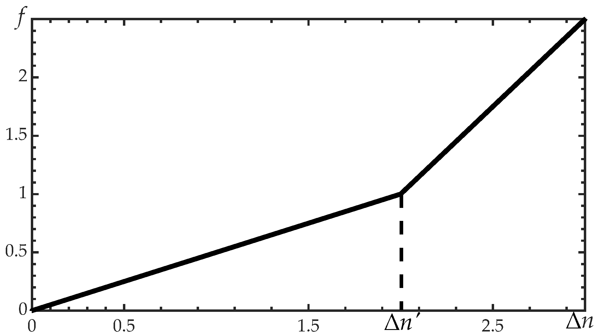
2.4. Annual Peak Shaving Cost of Power Generation Technology

The annual peak shaving cost (APSC) of power generation technology represents the equivalent cost incurred by the generator to reduce its own power generation ability through some technical means when there is a demand for peak shaving at the grid end. This cost includes the operating cost of making the unit lower than the rated output and the potential risk cost caused by the unit being in a peak shaving state. The peak shaving state of the unit is divided into conventional peak shaving and deep peak shaving. When the active power output of the unit falls below a certain threshold, the unit enters the deep peak shaving state, and the peak shaving cost will increase sharply [45,46]. This paper supposes that the peak shaving cost is a linear function of the peak shaving depth. Combined with the definition of CCI in Section 2.1, the APSC is expressed as a piecewise linear function of CCI.

In Figure 2, f represents the APSC, Δn is the difference between the actual CCI and the rated CCI, and Δn′ is the boundary between conventional peak shaving and deep peak shaving. When Δn is greater than Δn′, the peak shaving cost increases sharply, and the corresponding second half of the function curve has a larger slope.

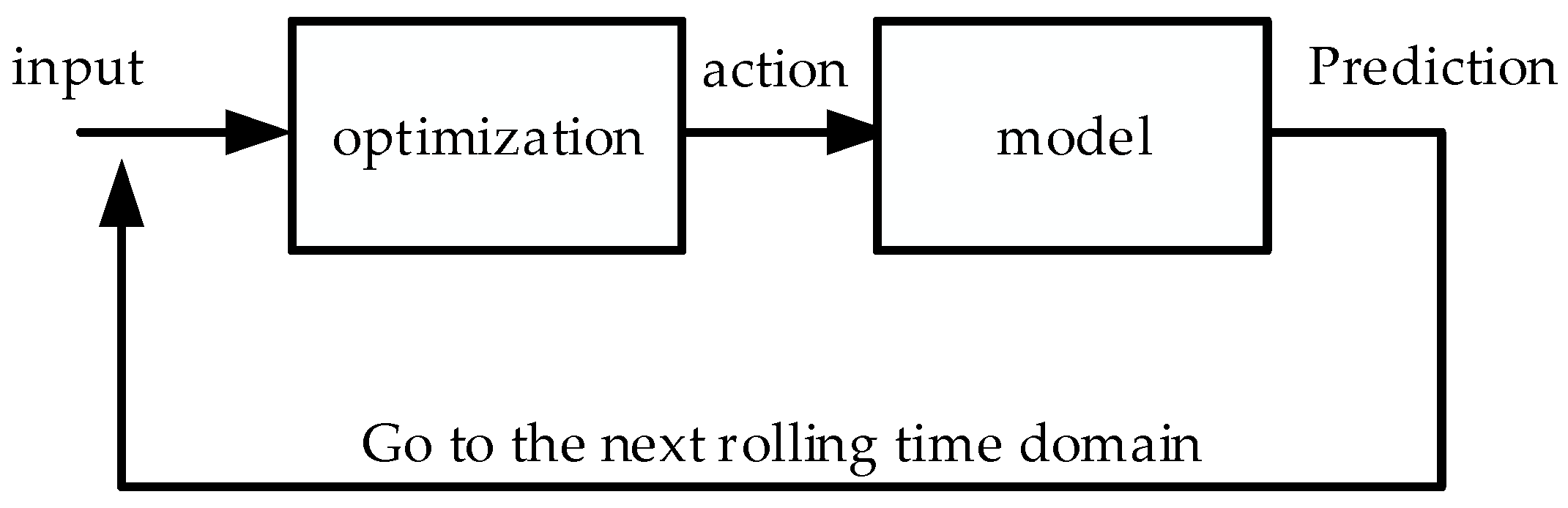
3. Two-Layer Optimization Model Based on MPC

3.1. Necessity and Basic Architecture of Model

The low-carbon evolution of the power supply structure is a long-term planning problem. Most of the traditional planning methods belong to the category of static planning, and the planning scheme cannot be adjusted in time for different states. The MPC dynamic planning algorithm decomposes the long-term planning problem into multiple rolling time domains and optimize them separately. The planning strategy is adjusted in time for different states so as to obtain the optimal solution for the overall long-term planning. MPC has strong superiority in long-term planning problems. In addition, according to the operation characteristics of the power system, the expansion of installed capacity and the regulation of power generation under constant installed capacity are regarded as two stages. The first stage is the planning of the installed capacity, which is generally pre-planned based on historical experience and economic factors, and the capacity value of the next time period is determined in advance for power plant construction. The second stage is operation regulation. On the basis of the existing installed capacity, the power generation of various power generation technologies is controlled separately considering several constraints so as to minimize the overall operating cost. According to this characteristic, this paper constructs the scientific problem as a two-layer optimization model and optimizes the installed capacity and power generation during the planning period.

The model proposed in this paper explores the relationship between power supply structure evolution and emission reduction targets considering the annual power balance, carbon emission reduction targets, and economic factors, and then obtains the optimal construction path for various units until 2030. This paper finds the optimal solution within the planning period using MPC and provides scientific support for the low-carbon transformation of the power industry in the future. The model covers six power generation technologies, including thermal power, hydropower, nuclear power, wind power, solar power, and other types of power (mainly biomass power). This paper discusses the option of carbon capture storage (CCS) technology, which is regarded as power generation technology with zero power. The minimum cost and minimum APSC for the planning period are the objective functions of the two-layer optimization model. Considering constraints such as power balance, resource constraints, and policy constraints, the optimal path for future power supply structure evolution is finally obtained. The model requires an input of planning starting point information, planning period, and correlated exogenous variables, such as the installed capacity, annual power generation, related costs, and emission parameters in the initial year. The added installed capacity and CCI of each power generation technology are variables to be optimized for the two-layer optimization problem, respectively.

3.2. Upper-Layer Installed Capacity Planning Model

In order to ensure the economy and low carbon emissions of the power generation side of the power system, the objective function of the upper optimization model is to minimize the sum of the construction cost, operation and maintenance cost, and carbon emission cost of the power generation side.

$$\min {\displaystyle \sum _{i\in N}{\displaystyle \sum _{j\in T}(C_{1i}^j+C_{2i}^j+C_{3i}^j)}},$$

(4)

where i is the label of different generation technologies, N is the number of all power generation technologies in this paper, j is the year relative to the starting year in the planning period, T is the planning period of each rolling time domain; and $C_{1i}^j$, $C_{2i}^j$, and $C_{3i}^j$ are the construction cost, operation and maintenance cost, and carbon emission cost of power generation technology i in year j, respectively, which are listed in Equation (5).

$$\begin{array}{l}{C}_{1i}^j=\Delta G_i^j\times C_{10i}^j\\ C_{2i}^j=G_i^j\times n_i^j\times C_{20i}^j\\ C_{3i}^j=G_i^j\times n_i^j\times e_i^j\times C_{30i}^j\end{array}$$

(5)

where $\Delta G_i^j$ is the added installed capacity of power generation technology i in year j, $n_i^j$ is the CCI of power generation technology i in year j; $e_i^j$ is the carbon emission coefficient of power generation technology i in year j, which represents the carbon emissions generated by the unit of electricity generated—for clean energy, $e_i^j=0$; and $C_{10i}^j$, $C_{20i}^j$, and $C_{30i}^j$ are the unit construction cost, unit operation and maintenance cost, and unit carbon emission cost of power generation technology I in year j, respectively.

(1) Constraints include the following. Annual installed capacity constraints.

$${\displaystyle \sum _{i\in N}{G}_i^j}\ge P_{peak}^j(1+\eta ),$$

(6)

where $G_i^j$ is the installed capacity of power generation technology i in year j, $P_{peak}^j$ is the peak load value in year j, and $\eta$ is the spare factor, which ensures that the total installed capacity per year is not lower than the peak load value of the year, and requires a certain safety margin.

(2) Annual power generation constraints.

$${\displaystyle \sum _{i\in N}{G}_i^j{n}_i^j}\ge W^j,$$

(7)

where $W^j$ is the total electricity demand of year j.

(3) Policy constraints. The proportion of the added installed capacity of some units every year should not be lower than a certain proportion, and this constraint reflects the government’s policy support for some power generation technologies.

$$\Delta G_i^j\ge p_i^j{\displaystyle \sum _{i\in N}\Delta G_i^j},$$

(8)

where $\Delta G_i^j$ is the added installed capacity of power generation technology i in year j; and $p_i^j$ is the minimum proportion of added installed capacity of power generation technology i in year j.

(4) Resource constraints.

$$G_i\le G_i^{\lim },$$

(9)

where $G_i^{\lim }$ is the maximum installed capacity of power generation technology i subject to natural resource constraints.

(5) Power supply constraints. This constraint means that the maximum power generation capacity of the units that can generate stable power must meet a certain proportion to prevent insufficient power supply due to the uncertainty of renewable energy.

$${\displaystyle \sum _{i\in N}{G}_i^j}{n}_{\max }{}_i^j\ge W^j\times {\delta }^j,$$

(10)

where $n_{\max }{}_i^j$ is the maximum CCI of power generation technology i in the year j, and ${\delta }^j$ is the minimum proportion of stable power generation that meets the security of power supply.

3.3. Lower-Layer CCI Optimization Model

After the installed capacity of each power generation technology is determined, the lower layer performs CCI optimization considering the power balance, and the objective function is to minimize the APSC as

$${\displaystyle \sum _{i\in N’}{f}_i^j=\{\begin{array}{c}{k}_1{}_i^j(n_{\max }{}_i^j-n_i^j),n{’}_i^j<n_i^j<n_{\max }{}_i^j\\ k_2{}_i^j(n_{\max }{}_i^j-n_i^j)+a_i,n_i^j<n{’}_i^j\end{array}},$$

(11)

where $f_i^j$ is the cost function of power generation technology i caused by peak shaving in the year j; $n_i^j$ is the CCI value of power generator i in the year j; $n{’}_i^j$ is the boundary CCI value between traditional peak shaving and deep peak shaving; $n_{\max }{}_i^j$ is the maximum CCI value of power generation technology i in year j; $k_1{}_i^j$ and $k_2{}_i^j$ are the cost coefficients corresponding to different peak shaving states, respectively, satisfying $k_2{}_i^j>k_1{}_i^j$; and $a_i$ is a constant term introduced to ensure the continuity of the function. Considering the uncontrollability of renewable energy generation technologies, the CCI of wind or solar power cannot be regarded as the variable to be optimized by the model, but is obtained by the prediction method in Section 2.2. Therefore, $N’$ in Equation (11) represents the aggregate of all power generation technologies, excluding wind and solar power generation.

Constraints are the annual power balance constraints as

$${\displaystyle \sum _{i\in N}{G}_i^j{n}_i^j}=W^j,$$

(12)

the meanings of physical quantities in Equation (12) are the same as those in Equation (7).

3.4. Model Solution

MPC is a special kind of control that obtains the optimal solution by solving a finite-time optimal control problem. The obtained optimal solution only works in the control process of the next period. This paper combines traditional power planning methods with MPC algorithms. Each rolling time domain of the MPC framework is a two-layer optimization problem of the power supply structure under static planning, and the optimal solution obtained is used as the control signal to determine the next rolling time domain of the MPC so as to carry out the next stage of optimization. In this way, each rolling time domain of the MPC is regarded as an optimization problem for different input signals, that is, to find the optimal control signal for different initial states, and realize the dynamic optimization of the power supply structure. This paper uses an MPC framework to solve the optimization model (established in Section 3.2 and Section 3.3) of a rolling time domain, obtains the optimal solution, and uses it as the input state of the next rolling time domain. The calculation principle of the MPC framework is shown in Figure 3.

This paper solves the proposed problem in accordance with the principle of MPC. The state variables of the model are the year, the annual installed capacity of power generation technologies and CCS devices, the added installed capacity, the CCI value of various power generation technologies, the annual carbon emissions, the cumulative carbon emissions, and the cumulative cost during the planning period. The state vector consists of several vectors, as listed in Equation (13).

$$\begin{array}{l}\mathit{G}=[\{G_i|i=1,2,\dots ,7\}]=[G_1;G_2;G_3;G_4;G_5;G_6;G_7]\\ \mathsf{\Delta }\mathit{G}=[\{\Delta G_i|i=1,2,\dots ,7\}]=[\mathsf{\Delta }{G}_1;\Delta G_2;\Delta G_3;\Delta G_4;\Delta G_5;\Delta G_6;\Delta G_7]\\ \mathit{n}=[\{n_i|i=1,2,\dots ,6\}]=[n_1;n_2;n_3;n_4;n_5;n_6]\end{array}$$

(13)

where i = 1, 2, …,7 are the labels of thermal power, hydropower, nuclear power, wind power, solar power, other types of power (mainly biomass power), and CCS, respectively. Equation (14) shows the state vector of this model.

$$\mathit{x}=[t;\mathit{G};\Delta \mathit{G};\mathit{n};em;E;J],$$

(14)

where t is the year relative to the initial year, em is the annual carbon emissions, E is the cumulative carbon emissions, and J is the cumulative cost during the planning period.

The control variable is the added installed capacity, which determines the total capacity in the next year. The control vector of MPC is expressed as Equation (15).

$${\mathit{u}}^j=\mathsf{\Delta }{\mathit{G}}^{j+1},$$

(15)

where j is the year relative to the starting year in each planning period. In addition, the MPC framework has the following constraints.

$$G_i^{j+1}=G_i^j+\Delta G_i^{j+1},$$

(16)

$$E^{j+1}=E^j+e{m}^{j+1},$$

(17)

$$J^{j+1}=J^j+{\displaystyle \sum _{i\in N}{\displaystyle \sum _{j\in T}(C_{1i}^{j+1}+C_{2i}^{j+1}+C_{3i}^{j+1})}},$$

(18)

Equations (16)–(18) are determined by their own physical meaning, and the calculation method of carbon emissions is shown in Equation (19).

$$e{m}^j={\displaystyle \sum _{i\in N}{G}_i^j{n}_i^j{e}_i^j},$$

(19)

where $e_i^j$ is the carbon emission coefficient of power generation technology i in the year j, and $e{m}^j$ is carbon emission of power generation in the year j. Then, we rewrote the dynamics of the optimization model according to Equations (13)–(19):

$${\mathit{x}}^{j+1}=f({\mathit{x}}^j,{\mathit{u}}^j),\hspace{1em}\hspace{1em}\hspace{1em}{\mathit{x}}^1=\mathit{x}0,$$

(20)

where $\mathit{x}0$ is the initial value of the state vector in the initial year.

The specific calculation steps of MPC are as follows.

• Predict exogenous variables, including the carbon emission coefficient, various costs, annual electricity demand and peak load in a year, the CCI of wind and solar power generation, etc. The prediction methods of the exogenous variables are shown as follows:

  $$e^j=a\lg (j+b)+c,$$

  (21)

Equation (21) uses the logarithmic function of time to predict the future carbon emission coefficient, and a, b, and c are coefficients obtained by fitting the historical data.

$$\begin{array}{l}{C}^{j+1}=C^j\times (1+{\delta }_C^j)\\ W^{j+1}=W^j\times (1+{\delta }_W^j)\\ P_{peak}^{j+1}=P_{peak}^j\times (1+{\delta }_{P_{peak}}^j)\end{array}$$

(22)

where ${\delta }_C^j$, ${\delta }_W^j$, and ${\delta }_{P_{peak}}^j$ are the change rates of costs, annual electricity demand, and peak load in the year j, respectively. Based on the prediction method elaborated in Section 2.2, the CCIs of wind and solar power generation, i.e., $n_4$ and $n_5$, are regarded as predictable exogenous variables in the optimization process considering the uncertainty of renewable energy.

2.

Define k representing the number of loops, then enter the initial value of the state variable and set k = 1, ${\mathit{x}}_k^1=\mathit{x}0$;

3.

Solve the upper-layer optimization problem established in Section 3.2. After temporarily regarding the CCI value in the rolling time domain as a constant, we rewrote the variables in this optimization model with state variables. We then used the number in parentheses to denote the element label of the vector and summarized the equivalent reformulation as follows:

$$\begin{array}{ll}& \min {\mathit{x}}_k{(24)}^{T+1}\\ s.t.& {\mathit{x}}_k{}^{j+1}=f({\mathit{x}}_k{}^j,{\mathit{u}}_k{}^j)\\ & {\mathit{x}}_k^1=\mathit{x}{0}_k\\ & {\mathit{u}}_k(1,\dots ,7)={\mathit{x}}_k(9,\dots ,15)\end{array}$$

(23)

for other constraints in Section 3.2, the variables in the model can be replaced by state variables according to Equation (14), which are not repeated here. Through this step, we obtain $\Delta \mathit{G}$ of each year during the planning period; therefore, the installed capacity is obtained.

4.

Solve the lower-layer optimization problem established in Section 3.3. Based on the obtained G in step 3, solve the optimal CCI for each year according to the optimization model established in Section 3.3, and get the results to replace the elements ${\mathit{x}}_k{(16,\dots ,21)}^j$ of the state vector. It is worth noting that ${\mathit{x}}_{19}$ and ${\mathit{x}}_{20}$, i.e., $n_4$ and $n_5$, are exogenous variables, and the substitution process does not change their values;

5.

Determine if k is equal to the set number of cycles. If they are not equal, set k = k + 1, then take the state variable of the second year in the rolling time domain as the initial state variable, i.e., $\mathit{x}{0}_k={\mathit{x}}_{k-1}{}^2$, and return to step 3; if they are equal, stop the loop;

6.

Finally, we obtain k groups of optimal solution matrices from k loops, then take out the initial state vector in the solution matrix of the first loop and the second column vector in each matrix to form a new matrix A. The reformulated matrix is the final optimal solution from the MPC framework, and we obtain our results as Equation (24).

$$\begin{array}{l}{\mathit{G}}^j=\mathit{A}(2,\dots ,8,j)\\ {\mathit{W}}^j=\mathit{A}(9,\dots ,14,j).\ast \mathit{A}(16,\dots ,21,j)\\ e{m}^j=\mathit{A}(22,j)\end{array}$$

(24)

In Equation (24), * represents the multiplication of the elements at the corresponding positions of the two matrices, and the result obtained is a matrix with the exact same format as the original matrix. The model solution method of the MPC framework is summarized in Algorithm 1.

Algorithm 1. MPC framework

1: Predict exogenous variables.

2. Input: initial value of the state vector, planning period T, and the number of cycles.

3: if k = 1, then

4: Solve the upper-layer optimization model.

5: Solve the lower-layer optimization model, and obtain an optimal solution matrix.

6: Set $A(:,1)={\mathit{x}}_1^1$.

7: for k = 2, …, T + 1, do

8: Set $\mathit{A}(:,k)={\mathit{x}}_{k-1}^2$.

9: Solve the upper-layer optimization model for ${\mathit{x}}_k{}^1={\mathit{x}}_{k-1}^2$.

10: Solve the lower-layer optimization model, and obtain an optimal solution matrix.

11: return A, G, W, and em.

4. Case Study

4.1. Base Data

This paper takes China’s power industry as an example; the planning period is 10 years, and the initial year is 2020. The installed capacity, power generation, and carbon dioxide emissions data from 2009 to 2020 used in the case were from China’s National Bureau of Statistics, China Electricity Council, and reference [47], respectively. The relevant cost and parameter settings referred to the literature [19,24]. In 2020, China’s installed power capacity reached 2162.49 million kW, of which the thermal power installed capacity was 1177.94 million kW, accounting for 54.47% of the total installed capacity. Compared with previous years, the capacity of renewable energy power generation, such as wind and solar, has further increased, accounting for about 25%. The successive introduction of national low-carbon policies has curbed the large-scale expansion of thermal power units to a certain extent, resulting in a decline in the growth rate of carbon emissions in the power industry, but the total emissions are still rising. Although renewable energy power generation has increased compared with previous years, there is still a large gap with the power generation of thermal power plants. Nuclear power units have high requirements for regulation and operation methods, and their operational safety is an important factor restricting the large-scale construction of nuclear power plants [48]. Restricted by the natural environmental and human factors, the growth rate of the hydropower installed capacity has gradually decreased [49]. Figure 4 shows the installed capacity of different generation technologies from 2009–2020.

Considering the availability of data and the complexity of the model, the simulation made the following assumptions.

• Carbon dioxide emissions in the power industry only come from thermal power units, ignoring the impact of transportation and thermodynamics on carbon emissions in the power industry;
• The installed capacity data in the past years all meet the load peak requirements and can be used as the lower limit constraint value of the installed capacity in the past years;
• Considering the improvement in the tolerance of the thermal power reserve due to technological progress, the minimum power generation ratio of the units that generate stable power decreases by an equal rate of change;
• Peak load and annual electricity demand increase in equal proportions;
• Ignoring increases in fuel costs due to energy shortages and political factors, all costs are subject to a fixed rate of change;
• The thermal power unit absorbs 90% of the carbon dioxide after a CCS retrofit.

Some parameters are listed in

Table A1. Change rate settings of cost.

Power Generation Technology	Unit Cost	Change Rate (%)
Thermal power	C10	−0.2
	C20	5
	C30	10
Hydropower	C10	1
	C20	0
	C30	0
Nuclear power	C10	−0.8
	C20	5
	C30	1
Wind power	C10	−2
	C20	−2.5
	C30	1
Solar power	C10	−5
	C20	−0.5
	C30	1
Others	C10	−1
	C20	−0.5
	C30	1

,

Table A2. Boundary value between the two peak shaving states and cost coefficients.

Power Generation Technology	n′ (h)	k1	k2
Thermal power	4540	1	5
Hydropower	3300	2	6
Nuclear power	7000	7	8
Others	4700	3	4

and

Table A3. Forecasting parameters of power demand.

Parameter	Initial Value (million kW/billion kWh)	Change Rate (%)
Ppeak	2162.49	3
W	7317.00	6

in Appendix A, which are important to the research, and

Table 1. Some cost parameters of the initial year.

Power Generation Technology	C10 (yuan/kW) 1	C20 (yuan/kWh) 1	C30 (yuan/tCO2) 1
Thermal power	5520	310.5	82.8
Nuclear power	19,320	172.5	0
Wind power	7719	103.5	0
Solar power	4485	69	0

¹ The cost unit yuan is RMB.

shows some of the cost parameters of the initial year.

For power generation technologies that have no emissions, the carbon emission coefficient is zero. Considering technological advancements, the carbon emission coefficient of thermal power is regarded as a logarithmic function of time that gradually decreases with time. This paper obtains the function expression by the nonlinear regression of historical data, which is expressed as

$$e(j)=-38.17\lg (j+12)+955.52,$$

(25)

where $e(j)$ is the carbon emission coefficient of thermal power in the year j. The unit of $e(j)$ is gCO₂/kWh.

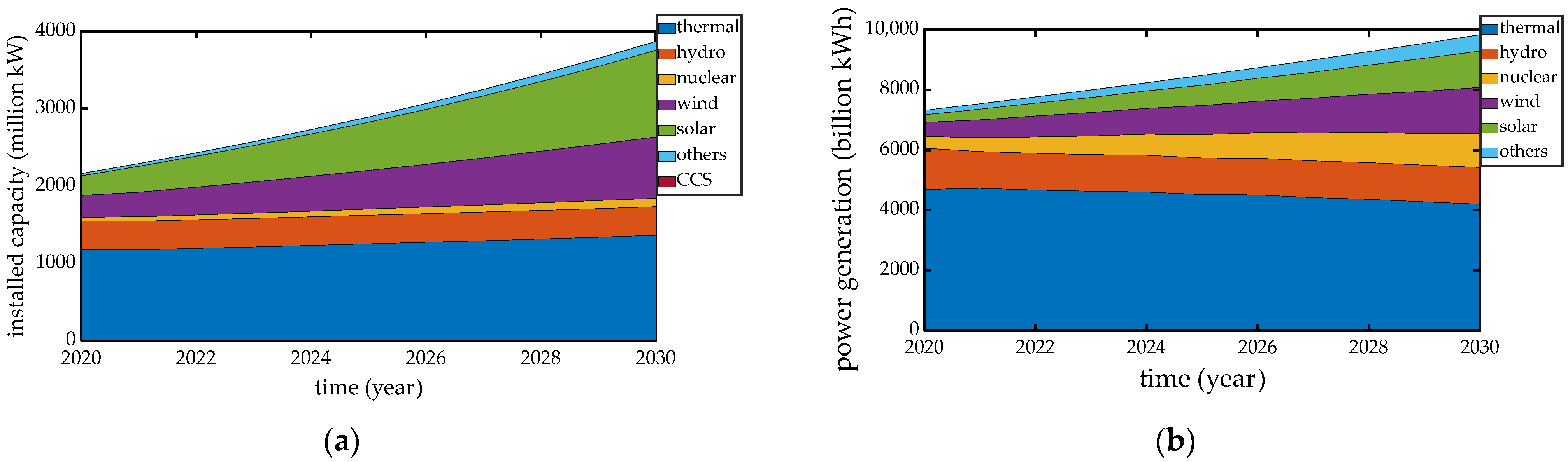
4.2. Results of the Case

In this case, we used CasADi, which came with IPOPT as an optimization solver, to solve the upper-layer optimization model, and used the interior point algorithm to solve the lower-layer optimization model. Finally, we obtained the following results in MATLAB.

(1) Predicted CCI of wind power and solar power generation.

According to historical data and the method proposed in Section 2.2 and Section 2.3, this paper assumed that the perturbation term ε of renewable power obeyed the normal distribution of N(0, 1602) and N(0, 2742) respectively, and then generated 100 sets of scenes. Figure 5 describes the scenes of the predicted CCIs of wind power and solar power generation, with each colored line representing an evolution scenario.

Then, we obtained the mean value of 100 sets of scenes as the prediction value of CCI, and we used this result to simulate the power generation ability of renewable energy in the future, as shown in

Table 2. The predicted CCIs of wind and solar power.

Time (Year)	CCIs of Wind Generation (h)	CCIs of Solar Generation (h)
2021	1847.886522	1016.125731
2022	1913.541309	1067.513049
2023	1902.93377	1057.050932
2024	1907.364856	1060.14718
2025	1865.555989	1041.880608
2026	1870.00318	1055.535528
2027	1882.558415	1079.256736
2028	1870.740671	1108.316839
2029	1878.5824	1080.04406
2030	1889.170836	1102.518975
2031	1867.022553	1154.598184
2032	1878.976875	1101.724634
2033	1911.402465	1139.257536
2034	1888.15016	1210.713959
2035	1876.303183	1148.691111
2036	1894.921912	1170.002537
2037	1904.653039	1147.8856
2038	1880.995522	1151.924091
2039	1904.351957	1148.916736
2040	1903.463496	1163.986872

.

(2) Optimal path of power supply structure.

The model solution results are shown in Figure 6. From the perspective of installed capacity, the installed capacity of renewable energy units continued to increase. The installed capacity of wind power could reach 794.59 million kW in 2030, accounting for 20.5% of the total installed capacity, with solar power generation reaching 1120.86 million kW, accounting for 28.94%. The growth rates will reach 182.2% and 342.28% respectively. Obviously, there will be a sharp increase in renewable energy units from 2020 to 2030. There will still be a small increase in thermal power units to meet the electricity demand, which will reach 1362.14 million kW in 2030, accounting for 35.17%. Although the installed capacity of thermal power units will increase, the proportion of thermal power units will drop a lot. In addition, due to limited natural resources, hydropower resources are relatively scarce, and the expansion of their installed capacity is no longer the first option. CCS equipment will not be applied on a large scale through economic incentives due to the high price.

In terms of annual power generation, the power generation of renewable energy units will increase significantly. In 2030, the annual power generation of wind power is expected to reach 1522.9 billion kWh, accounting for 15.5% of the total power generation, and the annual power generation of solar power will reach 1187.9 billion kWh, accounting for 12.1%. The thermal power generation capacity in 2030 will be 4519.1 billion kWh, accounting for 45.96% of the total power generation, and the power generation of other types of units will increase to a certain extent. In general, most of the electricity supply in 2030 will still originate from thermal power.

(3) Emission pathway of the power industry

With the large-scale expansion of renewable energy units in the future and the continuous reduction of the actual power generation of thermal power units, the carbon emissions of the power industry will reach a peak of 4.08 billion tCO₂ in 2023, and then drop gradually. As shown in Figure 7, there will be a slight drop in 2022 due to the expansion of renewable power generation, which means there is redundancy in thermal power generation at present. The carbon emissions of the power industry will peak earlier than the “carbon peak target”. From 2020 to 2030, the power industry will emit 44.23 billion tCO₂, which is still a considerable value.

5. Discussion

At present, the main way to reduce carbon emissions in the power system is to replace the original power generation from thermal power units with generation from renewable energy sources, such as wind energy and solar energy. Different power generation technologies play different roles in the power supply side. In order to achieve the “double carbon” goal, we should make every effort to ensure the share of renewable energy power generation, and reduce the abandonment of renewable energy as much as possible. In the future, thermal power units will be used more as a regulating power source to cope with the fluctuation of renewable energy power generation, smoothing the total active power output on the power source side.

Under the current technical conditions, the most reliable way to ensure the good regulation performance of the power system is to maintain sufficient reserve regulation capacity of thermal power units. Hydropower is affected by ecological, cultural, and natural factors, and its regulation performance is lower than that of thermal power units. As an energy storage power source, pumped storage power plants may become a new trend in the development of hydropower. The safety of nuclear power plants has always been a topic of debate. Especially after the Fukushima nuclear power plant accident, it became a power generation technology that was strongly resisted by the public. However, with the improvement of awareness of nuclear energy technology’s superiority and the improvement of nuclear energy control technology in recent years, nuclear power generation has once again become an important way to supply stable electric power and reduce carbon emissions.

Aiming at the operation stability and supply reliability, the power system still needs a certain proportion of thermal power units to provide the inertia level and adjustment capability when encountering disturbances. This is also the main reason why thermal power units cannot be quickly abandoned. The installation of CCS equipment in thermal power units may be a good choice, but, in addition to the higher construction and operation costs, the operation effect after installation is still unclear. Issues such as the transportation and storage of captured carbon dioxide also need further discussion. In some areas with a high proportion of thermal power, some thermal power units have been retrofitted for flexibility so that the active power output is significantly lower than the rated active power output. This is a method to reduce the carbon emissions of thermal power generation, but the reliability and security issues still require further study.

6. Conclusions

In view of the low-carbon transformation trend in the energy industry, this paper establishes a two-layer optimization model for the low-carbon evolution path of the power supply structure considering the fluctuation of renewable energy output and low-carbon transformation policies, and then uses the MPC framework to solve the problem. Finally, the optimal path for the evolution of China’s power supply structure from 2020 to 2030 is obtained. According to the results of the model solution, we obtained the main findings as follows.

(1) The carbon dioxide emissions of the power system in 2030 will decrease compared with those of 2020 and show a downward trend in the near future, but the total emissions will still be high. Due to the incentive effect of the “double carbon” goal on the low-carbon transformation of the power system, the carbon emissions of the power industry will reach a peak of 4.08 billion tCO₂ in 2023; after that, they will drop gradually. The carbon peak time of the power industry will be earlier than that promised by the “double carbon” goal, which means that the power industry needs to play a pioneering role in the realization of the “double carbon” goal in the future.

(2) Although the installed thermal power capacity will increase by 2030, power generation will decrease. Thermal power units will still play an irreplaceable role. In 2030, the installed capacity of thermal power plants will increase slightly compared with that in 2020, but its proportion will be reduced to only about 35.17%, which means that other types of power generation technologies will grow even more. The thermal power generation capacity in 2030 will be 4519.1 billion kWh, accounting for 45.96%, which is lower than that in 2020, indicating that, under the incentive of the “double carbon” goal, thermal power generation is no longer the first option to meet the power supply demand.

(3) Unlike thermal power units, both wind power units and solar power units have seen substantial increases in both installed capacity and annual power generation. Obviously, their proportions have also increased significantly. In 2030, the installed capacity of wind and solar power will reach 1915.45 million kW, accounting for nearly 50% of the total installed capacity. The annual power generation of wind and solar power is expected to reach 2710.8 billion kWh, accounting for 27.6% of the total power generation.

At present, the low-carbon transformation of the power industry is faced with two major difficulties. On the one hand, as one of the industries with the most carbon emissions, the power industry is facing huge pressure to reduce emissions, and the scarcity of fossil energy and its high emissions mean that thermal power units need to be phased out in the future. On the other hand, the large-scale expansion of renewable energy units brings hidden dangers to the power supply security of the power system. The need to improve the output performance of renewable energy units is still an urgent problem to be solved in the power industry. In the example described in this paper, China’s power supply structure is further optimized from 2020 to 2030, and the carbon emissions of the power industry will gradually decline after reaching the peak. With the development of renewable energy regulation technology and the improvement of traditional energy utilization efficiency in the future, the power system will gradually increase the proportion of renewable energy power generation under the premise of stable power supply and finally achieve the goal of carbon neutrality. Finally, the method proposed in this paper can effectively solve the optimal path of the low-carbon evolution of the power supply structure, which is of great significance for future power supply security, national economic development, and the realization of the “double carbon” goal.

References

1. Godde, C.M.; Mason-D’Croz, D.; Mayberry, D.E.; Thornton, P.K.; Herrero, M. Impacts of climate change on the livestock food supply chain; a review of the evidence. Glob. Food Secur. 2021, 28, 100488. [Google Scholar] [CrossRef] [PubMed]
2. Lu, S.B.; Bai, X.; Li, W.; Wang, N. Impacts of climate change on water resources and grain production. Technol. Forecast. Soc. Chang. 2019, 143, 76–84. [Google Scholar] [CrossRef]
3. Altieri, M.A.; Nicholls, C.I. The adaptation and mitigation potential of traditional agriculture in a changing climate. Clim. Chang. 2017, 140, 33–45. [Google Scholar] [CrossRef]
4. Cuthbert, M.O.; Gleeson, T.; Moosdorf, N.; Befus, K.M.; Schneider, A.; Hartmann, J.; Lehner, B. Global patterns and dynamics of climate-groundwater interactions. Nat. Clim. Chang. 2019, 9, 137–141. [Google Scholar] [CrossRef]
5. Wanders, N.; Wada, Y. Human and climate impacts on the 21st century hydrological drought. J. Hydrol. 2015, 526, 208–220. [Google Scholar] [CrossRef]
6. Alfieri, L.; Burek, P.; Feyen, L.; Forzieri, G. Global warming increases the frequency of river floods in Europe. Hydrol. Earth Syst. Sci. 2015, 19, 2247–2260. [Google Scholar] [CrossRef] [Green Version]
7. Simpson, N.P.; Mach, K.J.; Constable, A.; Hess, J.; Hogarth, R.; Howden, M.; Lawrence, J.; Lempert, R.J.; Muccione, V.; Mackey, B.; et al. A framework for complex climate change risk assessment. One Earth 2021, 4, 489–501. [Google Scholar] [CrossRef]
8. Preston, B.J. The Influence of the Paris Agreement on Climate Litigation: Legal Obligations and Norms (Part I). J. Environ. Law 2021, 33, 1–32. [Google Scholar] [CrossRef]
9. Schleussner, C.-F.; Rogelj, J.; Schaeffer, M.; Lissner, T.; Licker, R.; Fischer, E.M.; Knutti, R.; Levermann, A.; Frieler, K.; Hare, W. Science and policy characteristics of the Paris Agreement temperature goal. Nat. Clim. Chang. 2016, 6, 827–835. [Google Scholar] [CrossRef] [Green Version]
10. He, J.K. China’s INDC and non-fossil energy development. Adv. Clim. Chang. Res. 2015, 6, 210–215. [Google Scholar] [CrossRef]
11. Zhao, J.; Wang, J.Z.; Su, Z.Y. Power generation and renewable potential in China. Renew. Sustain. Energy Rev. 2014, 40, 727–740. [Google Scholar] [CrossRef]
12. Shuai, Y.; Zhao, B.; Jiang, D.; He, S.; Lyu, J.; Yue, G. Status and prospect of coal-fired high efficiency and clean power generation technology in China. Therm. Power Gener. 2022, 51, 1–10. [Google Scholar]
13. Jiang, Y.; Lei, Y.L.; Yan, X.; Yang, Y.Z. Employment impact assessment of carbon capture and storage (CCS) in China’s power sector based on input-output model. Environ. Sci. Pollut. Res. 2019, 26, 15665–15676. [Google Scholar] [CrossRef] [PubMed]
14. Tock, L.; Marechal, F. Environomic optimal design of power plants with CO2 capture. Int. J. Greenh. Gas Control 2015, 39, 245–255. [Google Scholar] [CrossRef]
15. Sifat, N.S.; Haseli, Y. A Critical Review of CO2 Capture Technologies and Prospects for Clean Power Generation. Energies 2019, 12, 4143. [Google Scholar] [CrossRef] [Green Version]
16. Sharma, A.K.; Thakur, N.S. Assessing the impact of small hydropower projects in Jammu and Kashmir: A study from north-western Himalayan region of India. Renew. Sustain. Energy Rev. 2017, 80, 679–693. [Google Scholar] [CrossRef]
17. Zelenakova, M.; Fijko, R.; Diaconu, D.C.; Remenakova, I. Environmental Impact of Small Hydro Power Plant-A Case Study. Environments 2018, 5, 12. [Google Scholar] [CrossRef] [Green Version]
18. Zeng, M.; Liu, Y.X.; Ouyang, S.J.; Shi, H.; Li, C.X. Nuclear energy in the Post-Fukushima Era: Research on the developments of the Chinese and worldwide nuclear power industries. Renew. Sustain. Energy Rev. 2016, 58, 147–156. [Google Scholar] [CrossRef] [Green Version]
19. IEA. World Energy Outlook 2021; OECD: Paris, France, 2021. [Google Scholar] [CrossRef]
20. Zhao, Z.Y.; Zuo, J.A.; Fan, L.L.; Zillante, G. Impacts of renewable energy regulations on the structure of power generation in China—A critical analysis. Renew. Energy 2011, 36, 24–30. [Google Scholar] [CrossRef]
21. Wu, Q.L.; Peng, C.Y. Scenario Analysis of Carbon Emissions of China’s Electric Power Industry Up to 2030. Energies 2016, 9, 988. [Google Scholar] [CrossRef] [Green Version]
22. Shen, W.; Qiu, J.; Meng, K.; Chen, X.; Dong, Z.Y. Low-Carbon Electricity Network Transition Considering Retirement of Aging Coal Generators. IEEE Trans. Power Syst. 2020, 35, 4193–4205. [Google Scholar] [CrossRef]
23. Wu, J.J.; Tang, G.H.; Wang, R.; Sun, Y.W. Multi-Objective Optimization for China’s Power Carbon Emission Reduction by 2035. J. Therm. Sci. 2019, 28, 184–194. [Google Scholar] [CrossRef]
24. Li, Z.; Chen, S.; Dong, W.; Liu, P.; Du, E.; Ma, L.; He, J. Low Carbon Transition Pathway of Power Sector Under Carbon Emission Constraints. Proc. Chin. Soc. Electr. Eng. 2021, 41, 3987–4000. [Google Scholar] [CrossRef]
25. Shu, Y.; Zhang, L.; Zhang, Y.; Wang, Y.; Lu, G.; Yuan, B.; Xia, P. Carbon Peak and Carbon Neutrality Path for China’s Power Industry. Eng. Sci. 2021, 23, 1–14. [Google Scholar] [CrossRef]
26. Yao, X.L.; Lei, H.T.; Yang, L.L.; Shao, S.; Ahmed, D.; Ismaail, M. Low-carbon transformation of the regional electric power supply structure in China: A scenario analysis based on a bottom-up model with resource endowment constraints. Resour. Conserv. Recycl. 2021, 167, 105315. [Google Scholar] [CrossRef]
27. Mirjat, N.H.; Uqaili, M.A.; Harijan, K.; Walasai, G.D.; Mondal, M.A.H.; Sahin, H. Long-term electricity demand forecast and supply side scenarios for Pakistan (2015–2050): A LEAP model application for policy analysis. Energy 2018, 165, 512–526. [Google Scholar] [CrossRef]
28. Wang, B.; Wang, L.M.; Zhong, S.; Xiang, N.; Qu, Q.S. Low-Carbon Transformation of Electric System against Power Shortage in China: Policy Optimization. Energies 2022, 15, 1574. [Google Scholar] [CrossRef]
29. Yang, M.; Patino-Echeverri, D.; Yang, F.X. Wind power generation in China: Understanding the mismatch between capacity and generation. Renew. Energy 2012, 41, 145–151. [Google Scholar] [CrossRef]
30. Zhang, Y.; Wang, J.X.; Wang, X.F. Review on probabilistic forecasting of wind power generation. Renew. Sustain. Energy Rev. 2014, 32, 255–270. [Google Scholar] [CrossRef]
31. van der Meer, D.W.; Widen, J.; Munkhammar, J. Review on probabilistic forecasting of photovoltaic power production and electricity consumption. Renew. Sustain. Energy Rev. 2018, 81, 1484–1512. [Google Scholar] [CrossRef]
32. Zhao, L.J.; Nazir, M.S.; Nazir, H.; Abdalla, A.N. A review on proliferation of artificial intelligence in wind energy forecasting and instrumentation management. Environ. Sci. Pollut. Res. 2022, 29, 43690–43709. [Google Scholar] [CrossRef] [PubMed]
33. Alimohammadisagvand, B. Influence of Demand Response Actions on Thermal Comfort and Electricity Cost for Residential Houses. Article Dissertation, Aalto University, Espoo, Finland, 2018. [Google Scholar]
34. Alimohammadisagvand, B.; Jokisalo, J.; Sirén, K. The potential of predictive control in minimizing the electricity cost in a heat-pump heated residential house. In Proceedings of the 3rd IBPSA-England Conference BSO 2016, Great North Museum, Newcastle, UK, 12–14 September 2016. [Google Scholar]
35. Muratori, M.; Rizzoni, G. Residential Demand Response: Dynamic Energy Management and Time-Varying Electricity Pricing. IEEE Trans. Power Syst. 2016, 31, 1108–1117. [Google Scholar] [CrossRef]
36. de Siqueira, L.; Peng, W. Control strategy to smooth wind power output using battery energy storage system: A review. J. Energy Storage 2021, 35, 102252. [Google Scholar] [CrossRef]
37. Fan, M. A Novel Optimal Generation Dispatch Algorithm to Reduce the Uncertainty Impact of Renewable Energy. In Proceedings of the 2016 IEEE Power and Energy Society General Meeting (PESGM), Boston, MA, USA, 17–21 July 2016. [Google Scholar] [CrossRef]
38. Ye, L.; Lu, P.; Zhao, Y.; Dai, B.; Tang, Y. Review of Model Predictive Control for Power System With Large-scale Wind Power Grid-connected. Proc. Chin. Soc. Electr. Eng. 2021, 41, 6181–6197. [Google Scholar]
39. Shiroei, M.; Ranjbar, A.M.; Amraee, T. A functional model predictive control approach for power system load frequency control considering generation rate constraint. Int. Trans. Electr. Energy Syst. 2013, 23, 214–229. [Google Scholar] [CrossRef]
40. Zheng, Y.; Hill, D.J.; Meng, K.; Luo, F.J.; Dong, Z.Y. Optimal Short-term Power Dispatch Scheduling for a Wind Farm with Battery Energy Storage System. In Proceedings of the 9th IFAC Symposium on Control of Power and Energy Systems (CPES 2015), New Delhi, India, 9–11 December 2015. [Google Scholar] [CrossRef]
41. Vand, B.; Ruusu, R.; Hasan, A.; Delgado, B.M. Optimal management of energy sharing in a community of buildings using a model predictive control. Energy Convers. Manag. 2021, 239, 114178. [Google Scholar] [CrossRef]
42. Kellett, C.M.; Weller, S.R.; Faulwasser, T.; Grune, L.; Semmler, W. Feedback, dynamics, and optimal control in climate economics. Annu. Rev. Control 2019, 47, 7–20. [Google Scholar] [CrossRef] [Green Version]
43. Li, Q.; Wang, X.; Rong, S.A. Probabilistic Load Flow Method Based on Modified Latin Hypercube-Important Sampling. Energies 2018, 11, 3171. [Google Scholar] [CrossRef] [Green Version]
44. Zhao, W.; Chen, Y.Y.; Liu, J.K. Reliability sensitivity analysis using axis orthogonal importance Latin hypercube sampling method. Adv. Mech. Eng. 2019, 11. [Google Scholar] [CrossRef] [Green Version]
45. Tian, X.; Fan, C. Analysis of Deep Peak Regulation and Its Benefit of Thermal Units in Power System With Large Scale Wind Power Integrated. Power Syst. Technol. 2017, 41, 2255–2263. [Google Scholar]
46. Lin, L.; Xu, B.Q.; Xia, S.W. Multi-Angle Economic Analysis of Coal-Fired Units with Plasma Ignition and Oil Injection during Deep Peak Shaving in China. Appl. Sci. 2019, 9, 5399. [Google Scholar] [CrossRef] [Green Version]
47. Zhang, Y.; Zhang, N.; Dai, H.; Zhang, S.; Wu, X.; Xue, M. Model Construction and Pathways of Low-Carbon Transition of China’s Power System. Electr. Power 2021, 54, 1–11. [Google Scholar]
48. Wang, H.; Rong, J. Analysis on China’s Nuclear Energy Development Path under the Goal of Peaking Carbon Emissions and Achieving Carbon Neutrality. Electr. Power 2021, 54, 86–94. [Google Scholar]
49. Zhao, X.F.; Wu, L.; Qi, Y. The energy injustice of hydropower: Development, resettlement, and social exclusion at the Hongjiang and Wanmipo hydropower stations in China. Energy Res. Soc. Sci. 2020, 62, 101366. [Google Scholar] [CrossRef]
Figure 1. Principle of the LHS method (take L = 6 as an example).
Energies 15 04450 g001
Figure 2. The APSC function curve.
Energies 15 04450 g002
Figure 3. The calculation principle of MPC.
Energies 15 04450 g003
Figure 4. Installed capacity of China’s power supply structure from 2009–2020.
Energies 15 04450 g004
Figure 5. The scenes of the predicted CCIs of wind and solar power generation. (a) Predicted CCI of wind power generation; (b) Predicted CCI of solar power generation.
Energies 15 04450 g005
Figure 6. The model solution results. (a) Optimal path of installed capacity; (b) Optimal path of annual power generation.
Energies 15 04450 g006
Figure 7. Emission pathway of the power industry.
Energies 15 04450 g007