Abstract
This paper proposes centralized and distributed optimization models for V2G applications to provide frequency regulation in power systems and the electricity market. Battery degradation and dynamic usages such as driving period, driving distance, and multiple charging/discharging locations are modeled. The centralized V2G problem is formulated into the linear programming (LP) model by introducing two sets of slack variables. However, the centralized model encounters limitations such as privacy concerns, high complexity, and central failure issues. To overcome these limitations, the distributed optimal V2G model is developed by decomposing the centralized model into subproblems using the augmented Lagrangian relaxation (ALR) method. The alternating direction method of multipliers (ADMM) is used to solve the distributed V2G model iteratively. The proposed models are evaluated using real data from the Independent Electricity System Operator (IESO) Ontario, Canada. Simulation results show that the proposed models can aggregate EVs for frequency regulation; meanwhile, the owners can obtain monetary rewards. The simulation also shows that including battery degradation and dynamic usage increases the model accuracy. By using the proposed approaches, the high cost and the low efficiency power generation units for frequency regulation can be compensated or partially replaced by EVs, which will reduce the generation cost and greenhouse gas emissions.
1. Introduction
As an important function of ancillary services, frequency regulation plays a pivotal role in power system operation and control. Power generation must be controlled to continuously meet demand, and an imbalance will cause frequency deviation [1]. Traditionally, fast response power generators are used for frequency regulation [2], e.g., burning gas turbines [3] and peak hydro [4]. However, these generators are less efficient and high cost [5].
Controlled charging and discharging connected to power systems—known as V2G applications—can be used as an efficient and economical source for frequency regulation [6,7,8,9,10,11]. In addition, the response of charging and discharging is fast, which makes EVs ideal sources for frequency regulation. Therefore, effective frequency regulation models using EVs are highly needed [12,13]. Since the individual battery capacity of EVs is insignificant compared with conventional generators [14], aggregators can be used to coordinate and manage the participation of a large fleet of EVs [15,16,17].
The studies on models for frequency regulation can be classified into two categories: unidirectional and bidirectional approaches. In the unidirectional models, the frequency deviation can be regulated by controlling the charging power and periods, i.e., EVs are used as a controllable load [18]. In [19], a unidirectional model was developed to regulate the frequency variations, where a fuzzy controller was used to optimize the charging energy and provided a bidding scheme to the electricity market. In [20], an optimization algorithm was proposed to maximize the revenue of an aggregator, while the frequency was regulated by controlling the charging rate of EVs. The study in [21] considered EVs as a controllable load to compensate for the intermittency of the renewable energy resources and to provide a frequency regulation service.
The second category is also called V2G bidirectional regulation. In this case, both charging and discharging are controlled to maintain the frequency at a nominal value [22]. Under this approach, many V2G models have been developed for frequency regulation [23,24,25,26,27]. For example, EVs were used for primary frequency regulation in the Great Britain electric network [23]. A V2G control approach was developed in [24] for frequency regulation based on uncertain dispatch and regulation capacity. In [25], load control with the V2G application model was proposed to regulate the system frequency in the presence of intermittent renewable energy, and a particle swarm algorithm was used to tune the model parameters. The work in [26] applied a new approach to control charging/discharging for frequency and voltage regulation. Model predictive control was implemented in [27] for frequency regulation. An optimal V2G model considering the owner’s satisfaction and maximizing the aggregator’s profit was developed in [28] for frequency regulation.
However, the majority of the previous studies focus on the centralized V2G approach for frequency regulation, which requires the private information of owners [29]. In addition, the centralized models face the problems of central failure and high complexity in handling a large number of EVs. For example, in the centralized approach, one computer is used to solve the optimization model, which schedules all EVs’ charging/discharging activities for frequency regulation. If the computer fails, the whole system will crash, which causes the central failure problem.
To overcome these limitations, distributed optimization approaches, such as dual decomposition, alternating direction method of multipliers (ADMM), analytical target cascading, auxiliary problem principle, consensus, and innovation, optimality and condition decomposition among others, have been developed. [30]. These approaches are applied in power system operation and control, e.g., voltage regulation [31], economic dispatch of power generation [32], and energy management [33,34].
Nevertheless, the distributed models are not widely applied to V2G applications in frequency regulation. Furthermore, battery degradation should be considered since frequent charging/discharging of EVs can wear out the battery. Dynamic usage patterns, such as battery state of charge (), battery capacity, plug-in time, and driving/plug-in periods, should also be considered [35].
This study proposes both centralized and distributed optimal V2G models for frequency regulation. Dynamic usage patterns and battery degradation are modeled. The centralized model is used as the benchmark scenario. The distributed model is developed through the ALR, and the ADMM is used to solve the distributed model. Simulation results from the centralized model and distributed model are compared. The distributed model can provide frequency regulation with similar performance as the centralized model; furthermore, it overcomes the limitation of the centralized model.
The contribution of this work are summarized as follows:
- 1.
- Both centralized and distributed V2G models with consideration of dynamic usage and battery degradation cost are developed and quantitatively evaluated for frequency regulation. Using the proposed methods, expensive resources responding to frequency regulation can be partially replaced by EVs.
- 2.
- The proposed distributed V2G models can integrate a very large fleet of EVs, protect owners’ privacy, and cope with the central failure problem of any centralized models.
- 3.
- Dynamic usages such as driving and plug-in time/location are included in the V2G model, which better reflects the actual usage; therefore, the accuracy of the V2G model is improved.
- 4.
- A linear battery degradation cost model is developed and incorporated into the proposed V2G model. This linearized model is accurate and computationally efficient.
- 5.
- Two sets of parameters ( and ) are introduced to prevent undesired charging and discharging behavior, e.g., discharging to merely charging other EVs.
- 6.
- Due to the introduction of , , and slack variables , both centralized and distributed V2G problems are formulated as LP models. Otherwise, a mixed-integer optimization model is required, which is much more difficult to solve.
2. Methodology
2.1. System Architecture
Figure 1 shows the system architecture. The plug-in EVs are connected to the power distribution system. An aggregator contracts with both the system operator (electricity market) and owners. Specifically, the contract between an aggregator and the system operator specifies that the aggregator needs to schedule and aggregate charging or discharging energy to follow a reference signal. This reference signal is the energy required for frequency regulation, which is announced by the system operator. When the power system frequency is higher than the nominal frequency, the reference signal is positive, representing that the power generation is greater than the demand. In this situation, charging will be preferred. In contrast, when the power system frequency is lower, the reference signal is negative, and discharging will be preferred. The contract also specifies the reward (USD/kWh) that the aggregator can provide for the owners in a V2G for frequency regulation.
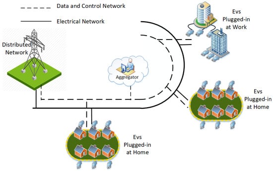
Figure 1.
V2G system architecture.
The aggregated charging/discharging may not track the frequency regulation reference signal exactly because of the dynamic usage of EVs, such as driving and limitation. The mismatch will be compensated for by the frequency regulation market. For example, PJM provides market-based compensation to resources that can adjust output or consumption in response to an automated frequency regulation signal [36]. Such resources in the PJM market include combustion turbines, hydro, storage, demand response, etc. PJM generates two different types of automated frequency regulation signals: Regulation A and Regulation D. Regulation A is a slow signal that is used to recover a larger, longer system frequency deviation. The Regulation D signal is a much faster, dynamic signal that needs resources to respond almost instantaneously. The resources that can respond almost instantaneously are extremely expensive and tend to be energy inefficient. Using the proposed method, such expensive resources can be partially replaced by EVs.
In the centralized approach, an aggregator collects data such as plug-in times, driving times, and . Based on the collected information, the aggregator solves the proposed centralized optimization model to match the frequency regulation signal. The model solution provides the scheduled charging and discharging profiles, which are used to control charging and discharging.
In contrast, in the distributed approach, each owner obtains global information, such as frequency regulation signals and the aggregated charging and discharging profile of the other EVs, from the aggregator. Based on this information, the schedules its charging and discharging energy by solving the proposed distributed optimization model. Through the coordination of the aggregator, a global optimal solution can be reached. Since each subproblem is much simpler than the centralized model, the distributed model can be solved more efficiently. Furthermore, owners do not need to share any information (e.g., driving periods, charging time, and daily energy consumption) with the other owners. They only need to share their charging/discharging profiles with the aggregator. The charging/discharging profiles are required to be shared with the aggregator for billing purposes anyways. Therefore, privacy can be preserved.
EVs can be plugged into the grid to provide the regulation service at both homes and workplaces. Both centralized and distributed V2G models incorporate dynamic usages and battery degradation cost.
We assume the communication infrastructure, such as power line communication, wireless communication, and ZigBee, is available [37]. We also assume the charging stations have bi-directional power flow and two-way communication capability.
2.2. Dyanmic Usage and Battery Degradation Cost
Figure 2 shows the dynamic driving and plug-in times. There are two driving periods: from home to workplace and from workplace to home . Due to similar daily routines, , , and tend to be normally distributed as follows [15].
where and represent the average and the standard deviation values, respectively, and x is the distance along the horizontal axis.
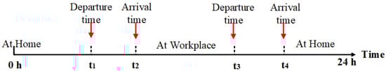
Figure 2.
driving and plug-in times in a day.
The battery consists of many lithium-ion cells and its capacity depends on the number of cells on it. Charging and discharging the battery over time, has a negative impact on this capacity. During charging and discharging, the ions move through the electrolyte and the two electrodes. Over time the physical structure of these components changes and causes a capacity loss. This process is called battery degradation [38].
Battery degradation cost can be modeled as follows [39]:
where is the battery purchasing cost in USD/kWh, and is the replacement cost. is the battery capacity. represents the depth of discharge; k is a constant value for the calibration purpose. The cycle life () expresses the lifetime of the battery based on the number of charging/discharging times before the capacity loss. The life cycle value relies mainly on the . More precisely, if the value is low, the battery degradation cost will decrease; hence the battery cycle life will increase. The relationship between and is as follows:
where represents the cycle life of the battery at 100 percent of DOD, while is the decay coefficient.
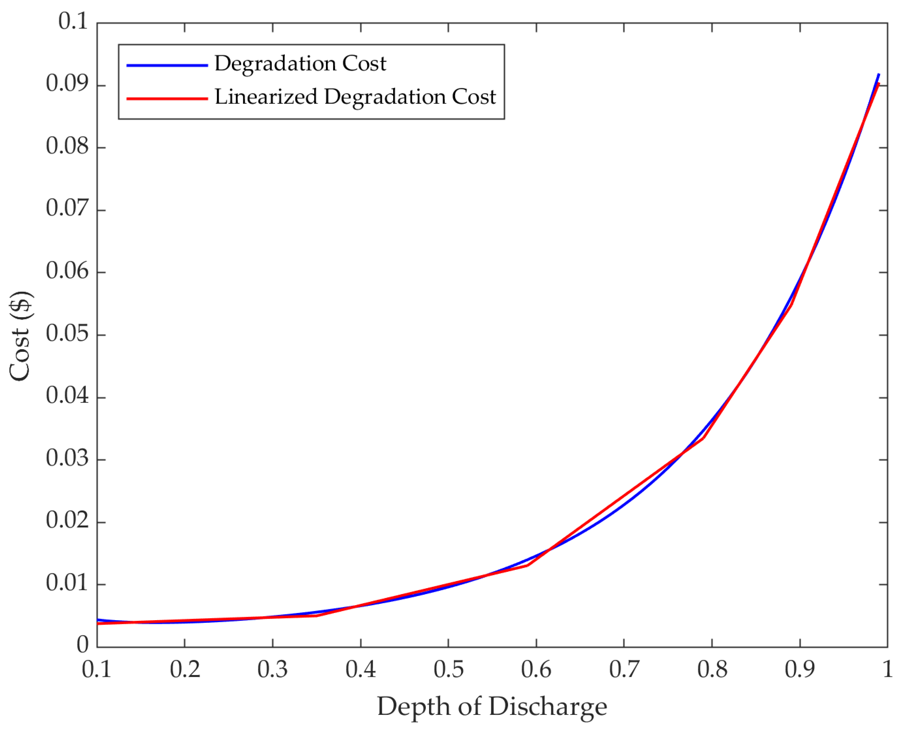
In the proposed V2G models, we incorporated the battery degradation cost. To reduce the computational complexity, we linearized the degradation cost by piecewise linear functions.
where and are constant.
In Figure 3, the blue line shows the degradation cost modeled by Equation (2), and the red line shows the linearized version modeled by Equation (4).
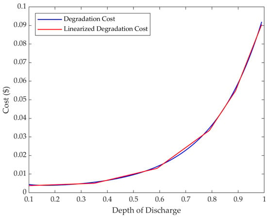
Figure 3.
Battery degradation cost.
2.3. Centralized V2G Model
The aggregator solves the following centralized model, and the charging and discharging signals from the optimal solution are used to control EVs. It is assumed that the aggregator has all the required information from EVs such as SOC, battery operation cost, and EV driving time.
subject to
In the objective function, Equation (5), M, and i represent the number of vehicles and the index of each vehicle, respectively; t is time, and T is the time horizon. In addition, is the operating power of batteries in which positive represents charging and negative represents discharging; is a set of slack variables to cancel the energy for driving. The reward for frequency regulation is given by the variable ; is a penalty coefficient, and is the degradation cost.
The cost for frequency regulation from the i-th at time t is represented by . The cost can be different among s depending on the preference of the owners and their satisfaction for participation in the frequency regulation program. For example, the cost of discharging an with 100% of is lower than that of an with 10% of .
The objective is to find a trade-off between maximizing the reward and minimizing the degradation cost.
Equation (6) illustrates the discharging constraint. Here, is the rated power, and is the plug-in time. Moreover, stands for needs discharging, which represents a set of time slots that the should be standing by or discharging. For example, when the load reference signal is negative, i.e., the system frequency is lower than the nominal frequency, s will be in the state of . For example, based on the frequency regulation signal, .
On the other hand, Equation (7) represents the charging limit. Here, stands for needs charging, which represents a set of time slots that the should be standing by or charging. For example, based on the frequency regulation signal, .
Both and are parameters which coordinate s to charge or discharge. These parameters can prevent undesired charging/discharging behavior. For example, some s discharge to merely charge other s.
In Equations (8) and (9), is the driving period. Here, is the battery capacity of the , and is the fraction of the battery capacity used for driving the i-th . Equation (8) is the energy consumption (discharging) for driving indicated by negative values. However, since the discharging does not provide energy to the power system, the discharging in this period should not be reflected in frequency regulation. Therefore, slack variables are introduced in Equation (9) and added into the objective to cancel the effect of during driving times.
Equation (10) calculates the through the time horizon for each , where represents the initial for each assuming that all s have the same initial values. Equation (11) illustrates the limits through the time horizon.
In Equations (12) and (13), is the accepted right before driving; and are the times to start driving. In other words, each vehicle should have a sufficient amount of energy for driving.
The in Equation (15) is the reference signal for frequency regulation; is the electrical power from/to the electricity market. The aggregated charging and discharging of the s and the electrical power from/to the electricity market should track . The aggregated charging/discharing may not exactly track the frequency regulation reference signal because of the dynamic usage of s such as driving and limitation. The mismatch will be absorbed by the electricity market. For example, the aggregator will purchase more energy from the electricity market when discharging cannot provide enough energy to track the reference signal. In contrast, when the charging cannot use the required energy, the electricity market will absorb the excess energy.
2.4. Distributed V2G Model
The centralized model requires private information to solve the optimization model. The owners generally hesitate to share this information, which can lead to an unsuccessful V2G application. In addition, the centralized model is not linearly scalable and has a central failure challenge. Moreover, it needs a central computer with a large memory and good computational capability to optimize a large number of s. Therefore, it is not suitable for large-scale networks.
In this section, we propose a distributed optimal V2G model to cope with such problems. In the distributed model, s (agents) solve their optimization problem locally while the global optimal solution is achieved.
As discussed in the previous section, Equation (15) illustrates the global constraint of the centralized model. This equation can be relaxed to decompose the optimization model into subproblems, and each subproblem can be solved by an (agent) and the electricity market (agent). In this case, the local information for each agent is used to solve these subproblems. Therefore, privacy can be preserved. In addition, the subproblem requires much less computational power. An ALR method is used to reform the centralized optimization model as follows.
subject to: Equations (6)–(14), where the weighted quadratic term makes the first derivative of the objective function continuous and its value is zero at the optimal point; is a penalty parameter.
This model can be decomposed into subproblems and solved by the ADMM [40] method in the decomposed manner. The i-th subproblem among M s is shown in Equation (17), and the one subproblem shown in (18) is for the electricity market. ThesSubproblem for the i-th is:
subject to: Equations (6)–(14).
Note that the term in Equation (16) is reduced to in Equation (17). This is because the terms and are constant numbers for the i-th and therefore can be ignored.
The subproblem for the electricity market is:
The ADMM algorithm is shown in Algorithm 1. In each iteration (), each agent (i) optimizes its own problem separately to obtain the and values These values are sorted according to their closest value to the average value which was obtained from the previous iterations. Then, the dual variable () is updated to be used in the next iteration. Once error () is equal to or less than a minimum value, the algorithm converges.
| Algorithm 1: ADMM Algorithm |
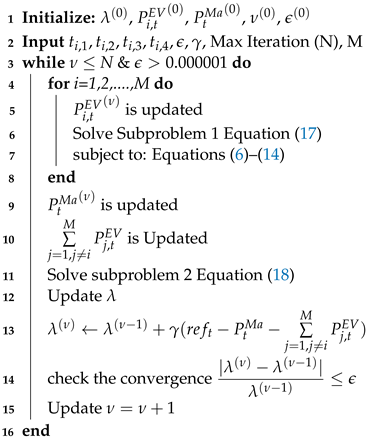 |
3. Simulation Results
This section presents the simulation results for the following scenarios. Scenario #5 has 500 s, and the rest of the scenarios have 50 s:
Scenario #1: This is our reference scenario, with no V2G for frequency regulation. The electricity market is solely responsible for frequency regulation.
Scenario #2: Centralized model.
Scenario #3: Centralized model with the central failure problem.
Scenario #4: Distributed model.
Scenario #5: Distributed model for a large number of s (500 s).
Scenario #6: Distributed model considering some s fail in the commitment for frequency regulation.
Scenario #7 Distributed model with degradation cost.
3.1. Experimental Setup
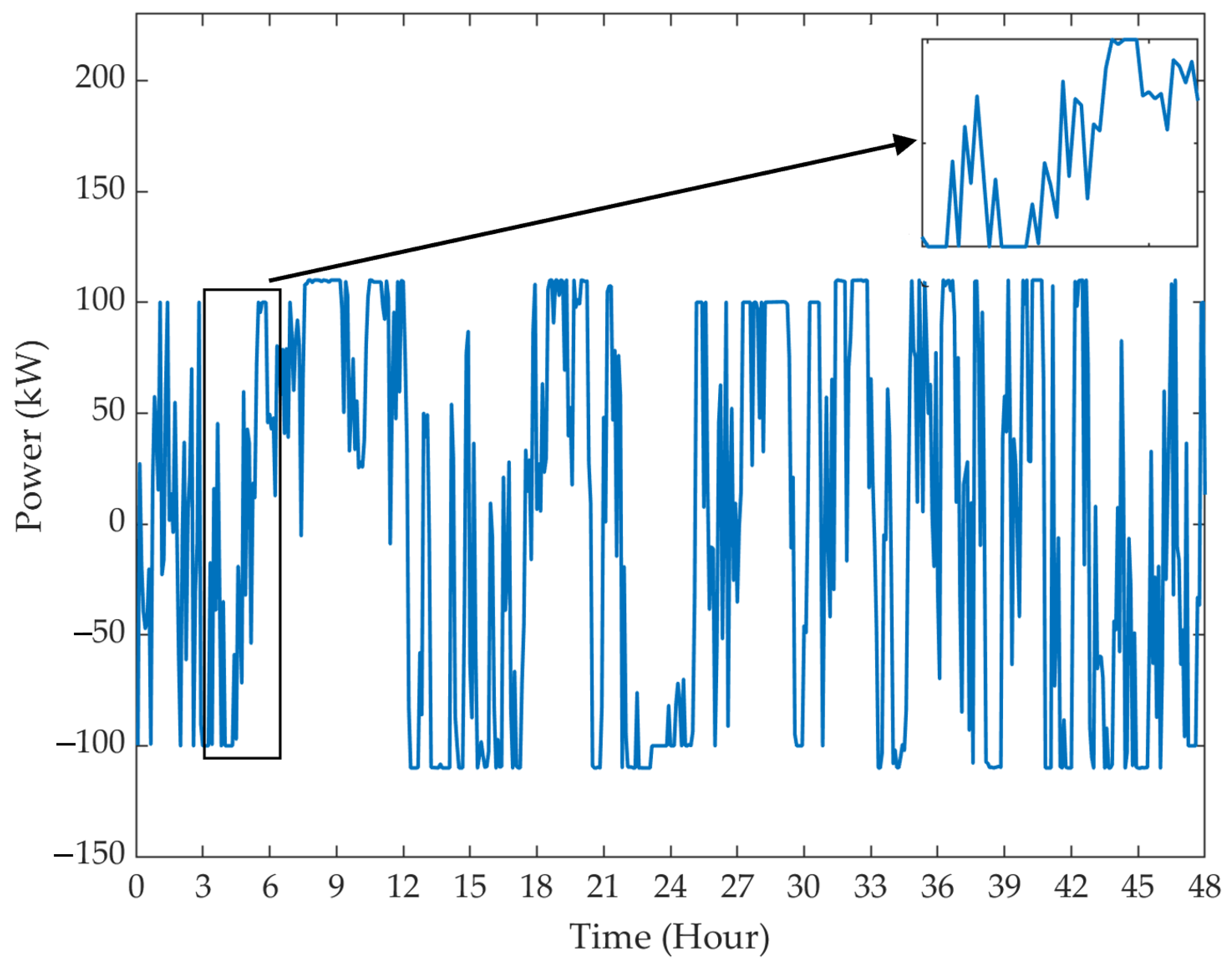
The distribution network was assumed to have 500 homes. Some of the households have s, i.e., there were 50 s. Nissan leaf e-plus with the capacity of 62 kWh was utilized in the proposed models. The frequency regulation data on 1 December 2017 to 2 December 2017 in the Ontario area from the Independent Electricity System Operator (IESO) [36] was used as the reference signal as shown in Figure 4. The aggregated charging and discharging was supposed to track this set of reference signals for frequency regulation.
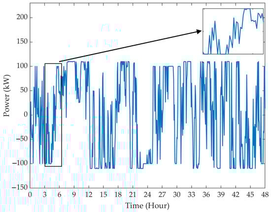
Figure 4.
Frequency regulation reference signal [36].
We conducted a two-day simulation and showed the results from 9 a.m. of the first day to 9 a.m. of the second day. Table 1 summarizes the major parameters. The time horizon was 48 h with a time interval of 5 min. s could be plugged in at both home and workplace with the rated charging/discharging power as 10 kW.
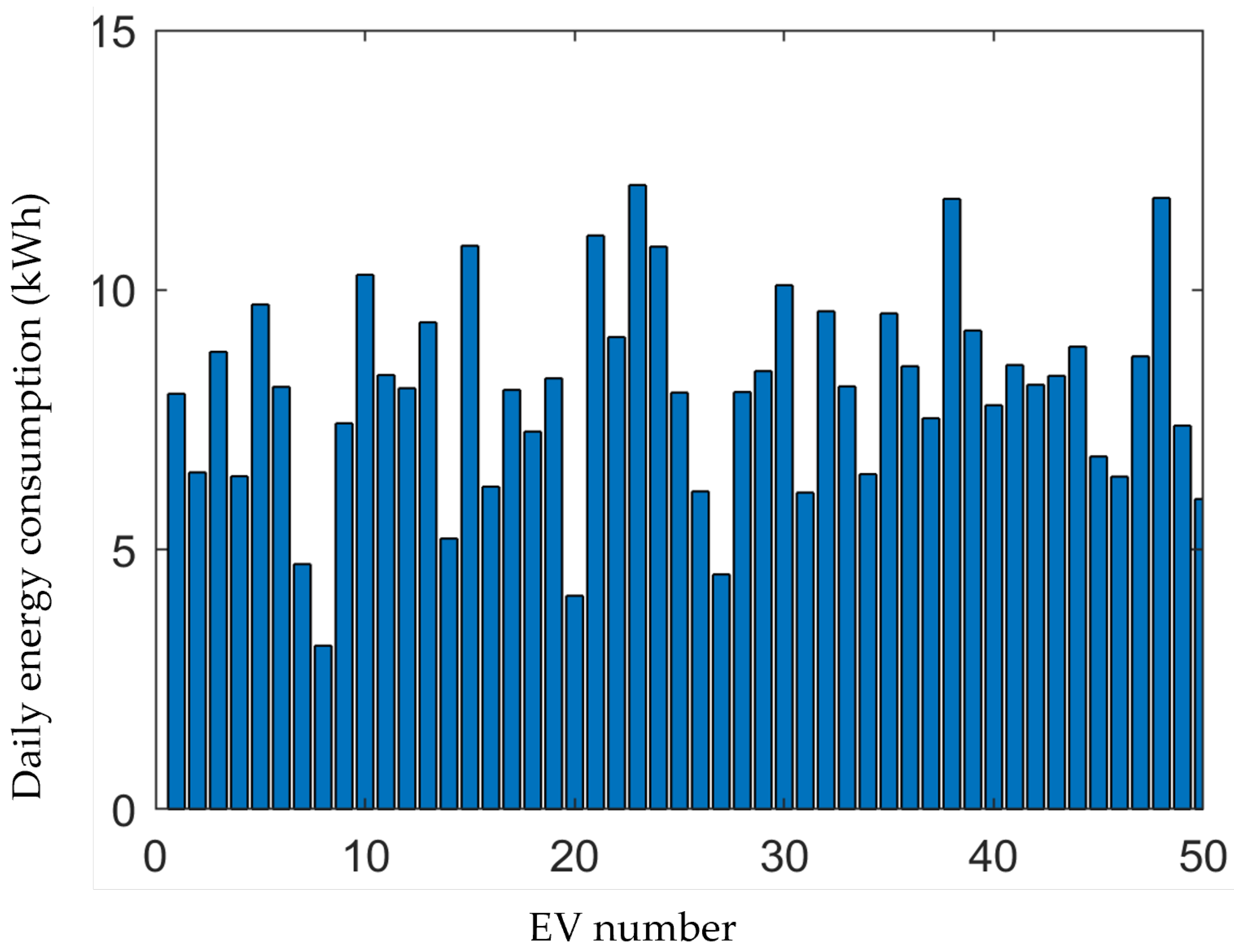
The daily energy consumption () for driving was calculated based on the daily driving distance () and energy consumption per km (), as follows.
Based on the studies in [15,41,42], we assumed that the daily driving distance follows a normal distribution. The average value was 30 km, and the standard deviation was 10 km. The average energy consumption per km was 0.2 kWh/km [43].
The daily energy consumption () can then be calculated based on Equation (19), which also follows a normal distribution. The average daily energy consumption was 8 kWh, and the standard deviation was 2 kWh. Figure 5 shows the bar chart of the daily energy consumption for 50 s.
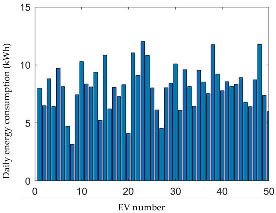
Figure 5.
Daily energy consumption.
The parameter can then be calculated as , where kWh for the Nissan leaf used in this study.
The parameters of the linearized degradation cost model are also shown in Table 1. The minimum and maximum were 0% and 100%. The initial was 50%, and the accepted before driving (at ) was 50%. The electricity market price for frequency regulation was 0.687 USD/kWh [44]. The charging cost was 0.14 USD/kWh [45]. The reward to owners because of participating in the V2G for frequency regulation was 0.3 USD/kWh [46]. The centralized and distributed models were solved using CVX with Mosek solver [47,48,49]. MATLAB 2020a was used to simulate all algorithms.

Table 1.
The main parameters.
The mean approximation percentage error (MAPE) and mean approximation error (MAE) were used to calculate how close the charging and discharging can track the reference signal. MAPE is shown in Equation (20) and MAE is shown in Equation (21) [51].
where and are the reference and model signals values, respectively, throughout the time horizon T.
In each scenario, we calculated the charging cost, the battery degradation cost, the reward from participating in the V2G, and the revenue. Although, the degradation cost was not included in the objective function in Scenarios #2–#6, we still calculated the degradation cost to show the fact. In Scenario #7, the degradation cost was included in the objective function.
3.2. Scenario #1: No V2G for Frequency Regulation
In Scenario #1, it is assumed that there is no s participating in frequency regulation. The electricity market is responsible for regulating the frequency deviation and match the reference signal. The electricity market adjusts the power generation to regulate the frequency. For example, in the PJM market, the regulation price includes capability and performance. The regulation capacity requires a resource to be available to provide this service and the regulation performance ensures that the resource can respond to frequency regulation signals [52]. In our study, we assume the regulation price was 0.687 USD/kWh [50]. The energy needed from the electricity based on the regulation signal shown in Figure 6 was 865 kWh. Then, the frequency regulation cost was calculated as USD 599.5.
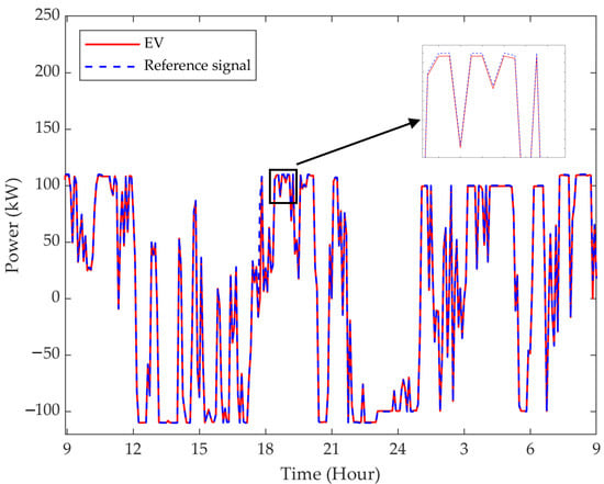
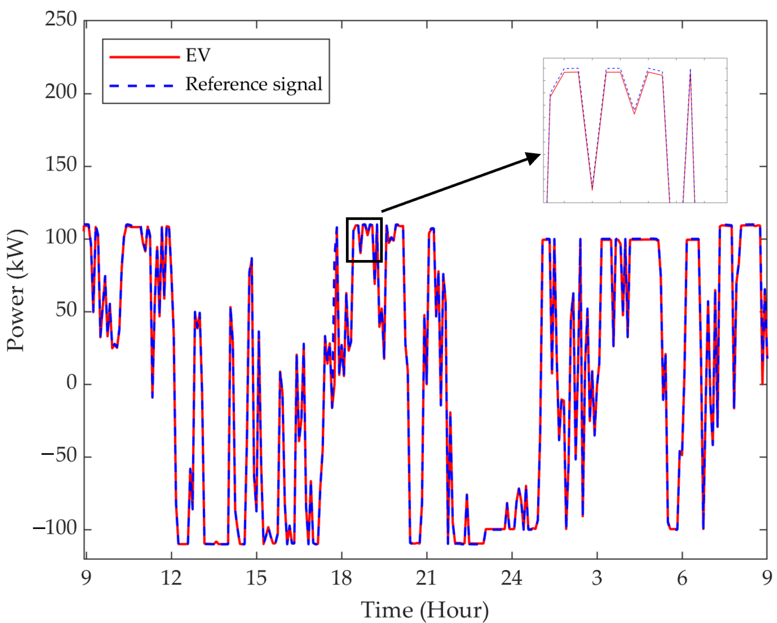
Figure 6.
Aggregated charging and discharging profile from 9 a.m. on the first day to 9 a.m. on the second day for frequency regulation in Scenario #2.
3.3. Scenario #2: Centralized Model
In this scenario, we implemented the centralized V2G model without including the battery degradation cost in the objective function (i.e., ). The charging and discharging of the s were optimized to maximize rewards and track the reference signal.
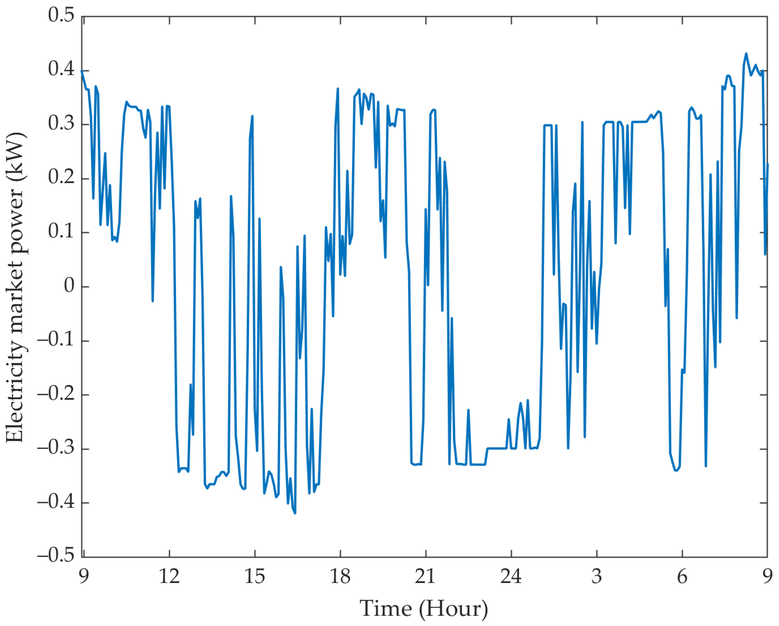
In Figure 6, the blue line shows the reference signal, which is the required energy for frequency regulation. The red line shows the aggregated charging and discharging energy. The aggregated charging and discharging were calculated from the centralized model. As can be seen, the aggregated charging and discharging were controlled to match the reference signal; however, there is a small mismatch due to the unavailability of s during driving periods as shown in Figure 6. The MAPE was 0.32%. and the MAE was 0.014 kW. This small mismatch was compensated for by the electricity market as shown in Figure 7.
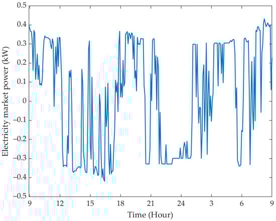
Figure 7.
Electricity market power profile to cover the mismatch between the reference signal and s power.
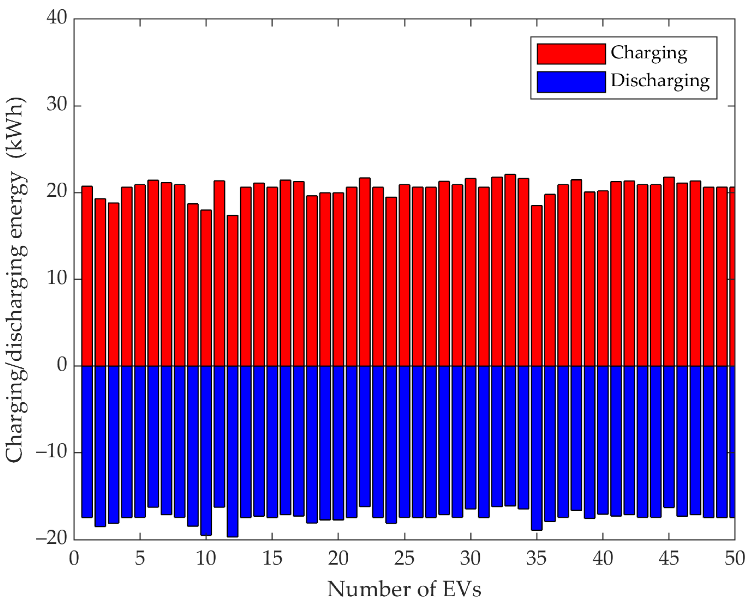
Figure 8 shows the individual charging and discharging energy from of the first day to of the second day.
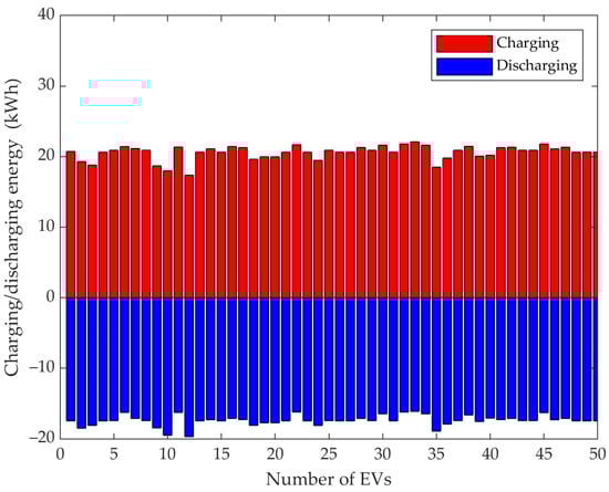
Figure 8.
Individual charging and discharging energy from on the first day to on the second day.
The charging cost was USD 158.08. The obtained rewards from V2G participation were USD 261.8. Although, the degradation cost was not incorporated into the objective function, we still calculated the degradation cost, which was USD 51.12. The revenue was then calculated as USD 52.59.
The main problem in this model is that it takes a long time to solve the optimization problem when we increase the number of s. Therefore, this method is not suitable for a large-scale network.
3.4. Scenario #3: Centralized Model with the Central Failure Problem
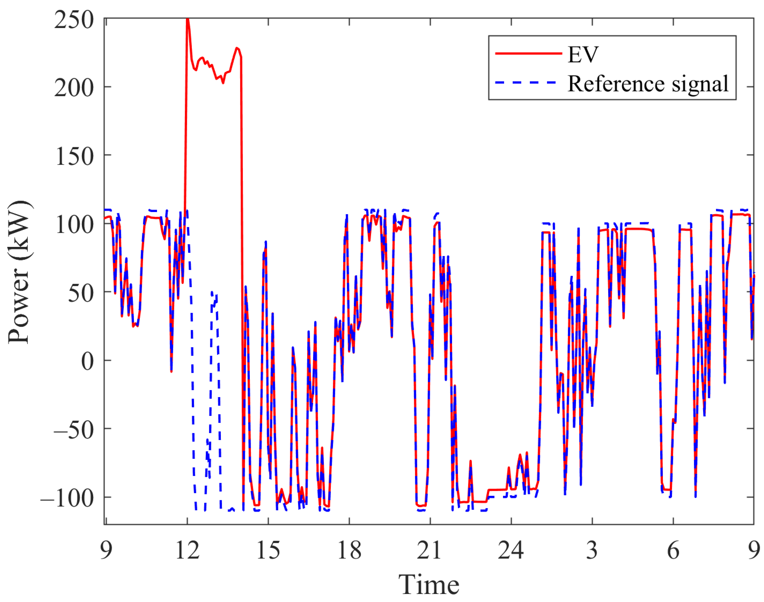
In this scenario, we assumed that there was a failure in the centralized model for two hours from 12:00 to 14:00 due to the breakdown of the computer or communication. Figure 9 shows the charging/discharging from 9 a.m. of the first day to 9 a.m. of the second day.

Figure 9.
Aggregated charging and discharging profile for frequency regulation with two hours failure to the centralized optimizer from 12:00 to 14:00 in Scenario #3.
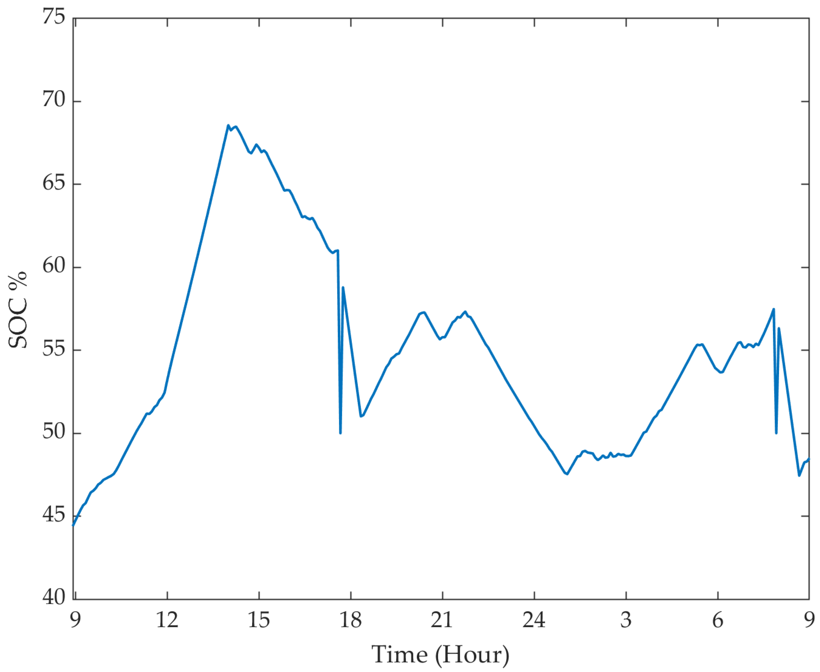
During this failure, due to the absence of control on s’ charging or discharging, s worked as a load; hence they charged their batteries. Furthermore, the behavior of s during this period increased the imbalance between demand and supply and hence increased the frequency deviation. Figure 10 shows the value of one for one day. It can be seen that the is increasing during the failure period.
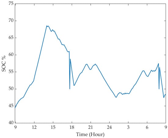
Figure 10.
percentage of one from 9 a.m. on the first day to 9 a.m. on the second day.
3.5. Scenario #4: Distributed Model
Although the centralized model shows a good performance in solving the frequency regulation problem, many drawbacks and limitations make it undesirable. These drawbacks include: (1) The centralized model sacrifices owners’ private information where each customer needs to provide the driving time, the driving periods, the plug-in time, the contracted rewards, and the battery . (2) The centralized model is unreliable for providing the frequency regulation service where one central computer is responsible for optimization and scheduling the charging and discharging power for each . Once there is a failure due to communication or any other reason, there will not be any control or regulation, as discussed in Scenario #3. (3) The centralized model has a mishandling problem for large-scale networks. In Scenario #4, the distributed model was developed to overcome these limitations and determine the optimal scheduling for the aggregated s to provide the frequency regulation. The degradation cost model was not considered in this scenario (i.e., ).
The subproblems were solved in parallel, which decreased the computational complexity. The ADMM was used to solve the model. Each was considered as an agent that solves its own optimization problem individually and locally.
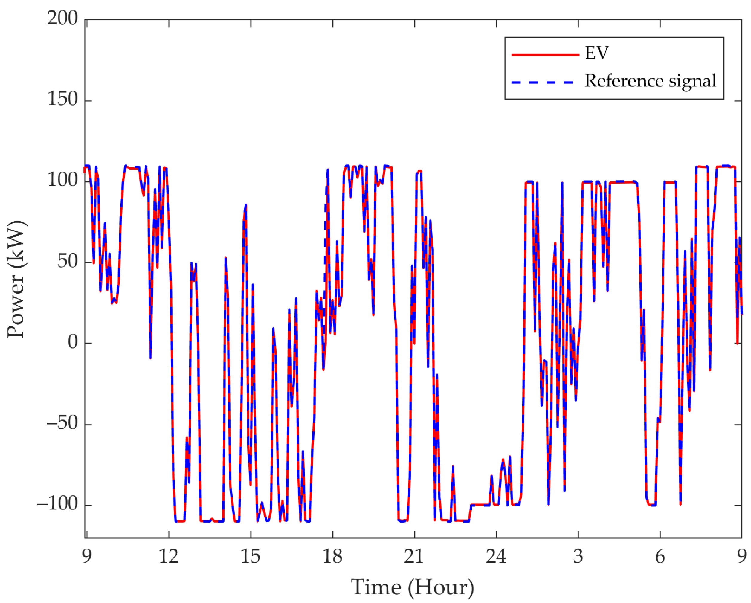
Figure 11 shows the charging and discharging power that follows the regulation reference signal. The MAPE was 0.028% and the MAE was 0.0067 kW. The small MAPE and MAE values show the mismatch between the charging/discharging profiles and the reference signals is very small. The small mismatch can be compensated for by the electricity market.
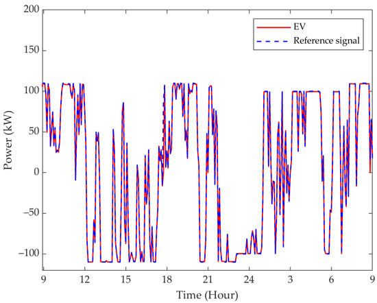
Figure 11.
Aggregated charging and discharging profile for frequency regulation in Scenario #4.
The charging cost was USD 158.55 and the battery degradation cost was USD 51.27. The obtained rewards from V2G participation was USD 262.57. The revenue was USD 52.75.
3.6. Scenario #5: Distributed Model for a Large Number of s
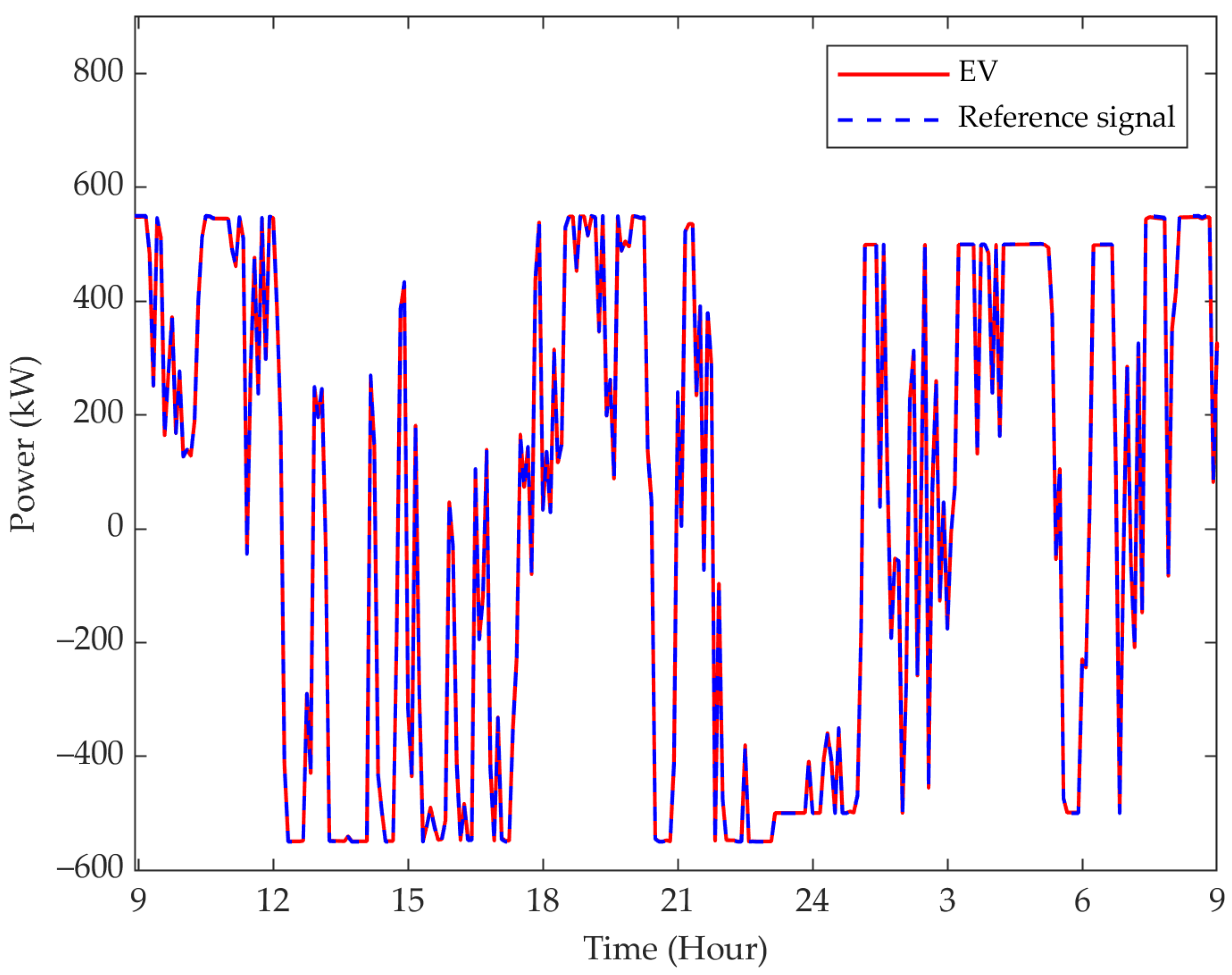
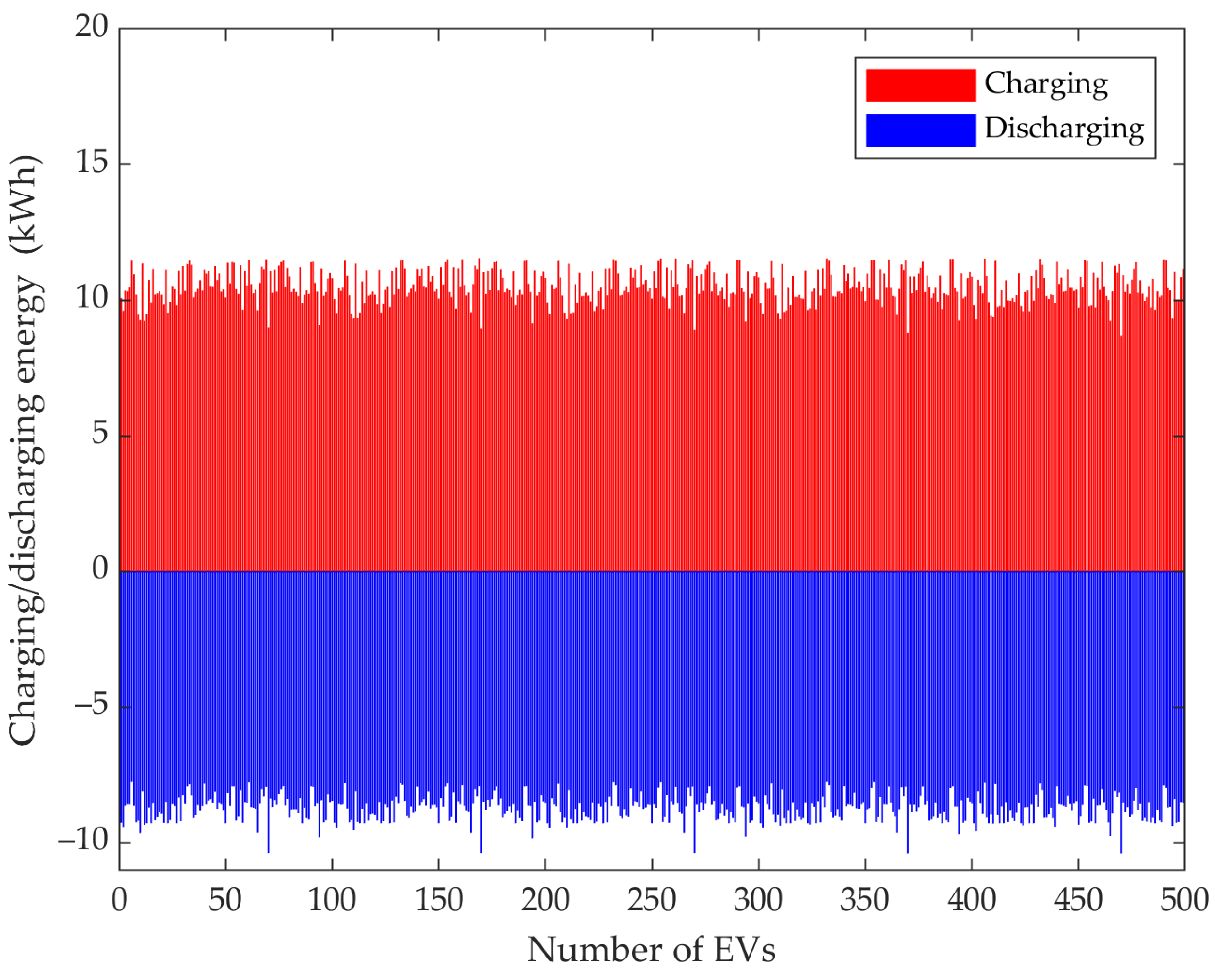
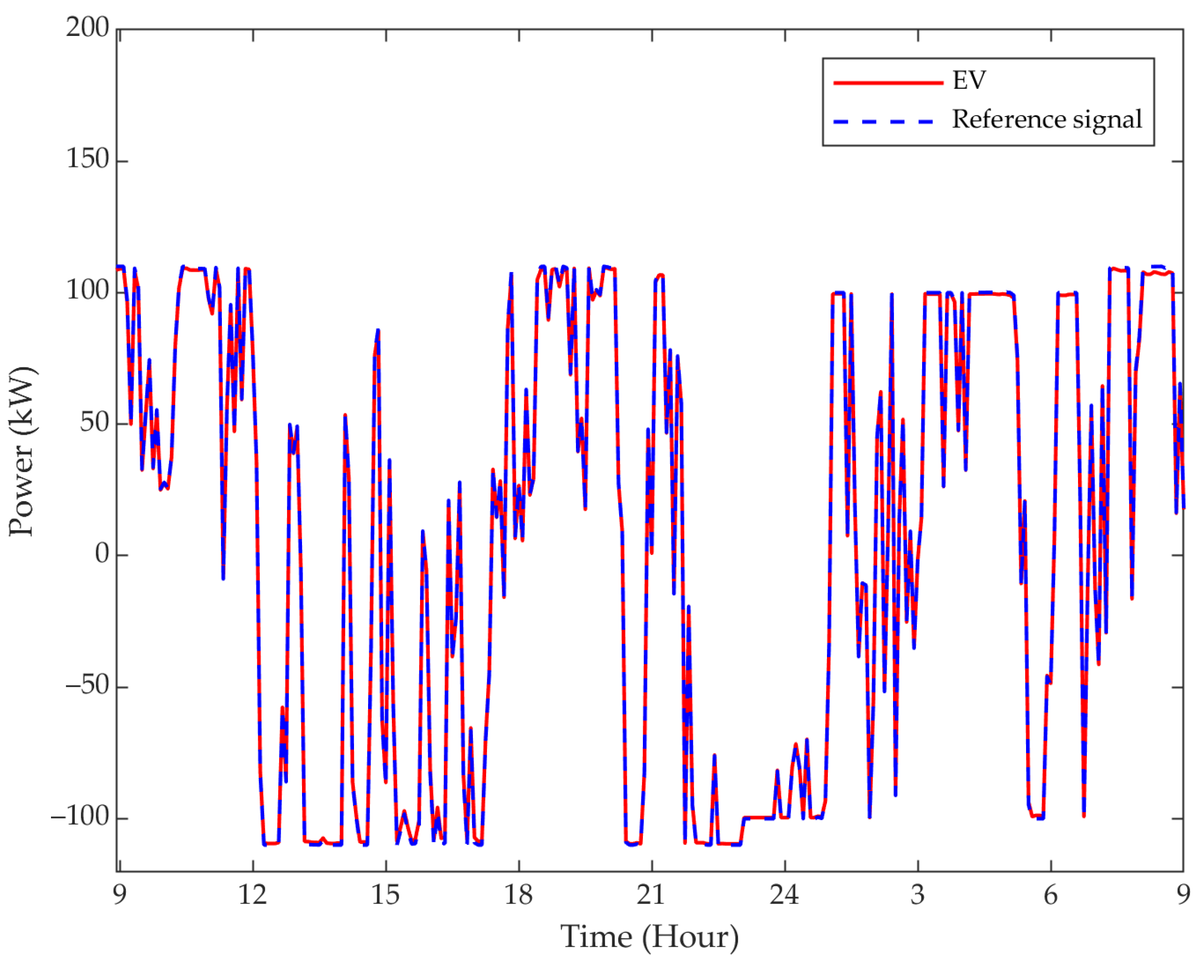
To check the power of the distributed model, we ran the same model with a large-scale network. To validate the proposed model with a high-scale network, the reference signal was scaled up, and 500 s were integrated into the distributed network. Figure 12 shows the regulation profile. Figure 13 shows the individual charging and discharging energy from on the first day to on the second day.
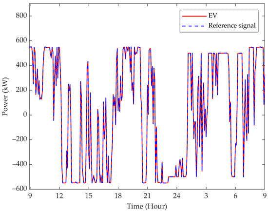
Figure 12.
The 500 s charging and discharging profile for frequency regulation in Scenario #5.
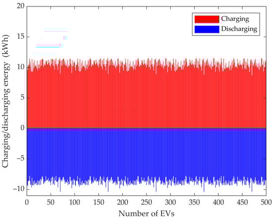
Figure 13.
Individual charging and discharging energy from on the first day to on the second day in Scenario #5.
3.7. Scenario #6: Distributed Model Considering Some s Fail in the Commitment
We assumed that 10 vehicles failed in their commitments due to the individual computer system failure or communication failure. Figure 14 shows the simulation results. As can be seen, the remaining 40 s could regulate the frequency and match the reference signal similar to the 50 s. The MAPE and MAE values were 0.83% and 0.11 kW, respectively.

Figure 14.
The 40 s charging and discharging profile for frequency regulation in Scenario #6.
3.8. Scenario #7 Distributed Model with Degradation Cost
In this scenario, we incorporated the battery degradation into the objective function to better reflect the reality because the battery is one of the most expensive and important components in s.
In the objective function (Equation (17)), is a penalty coefficient to find the trade-off between the reward and the battery degradation cost. More specifically, a small/large value of may decrease/increase the impact of the degradation cost on the objective function. Therefore, should be chosen carefully. Based on our previous work, was chosen [15].
Comparing the aggregated charging and discharging with the reference signal, the MAPE was 20% and the MAE was 0.57 kW. The electricity market could compensate for the mismatch.
The charging cost was USD 150.7, and the battery degradation cost was USD 49.3. The obtained rewards from V2G participation were USD 255.88. The revenue was USD 55.87.
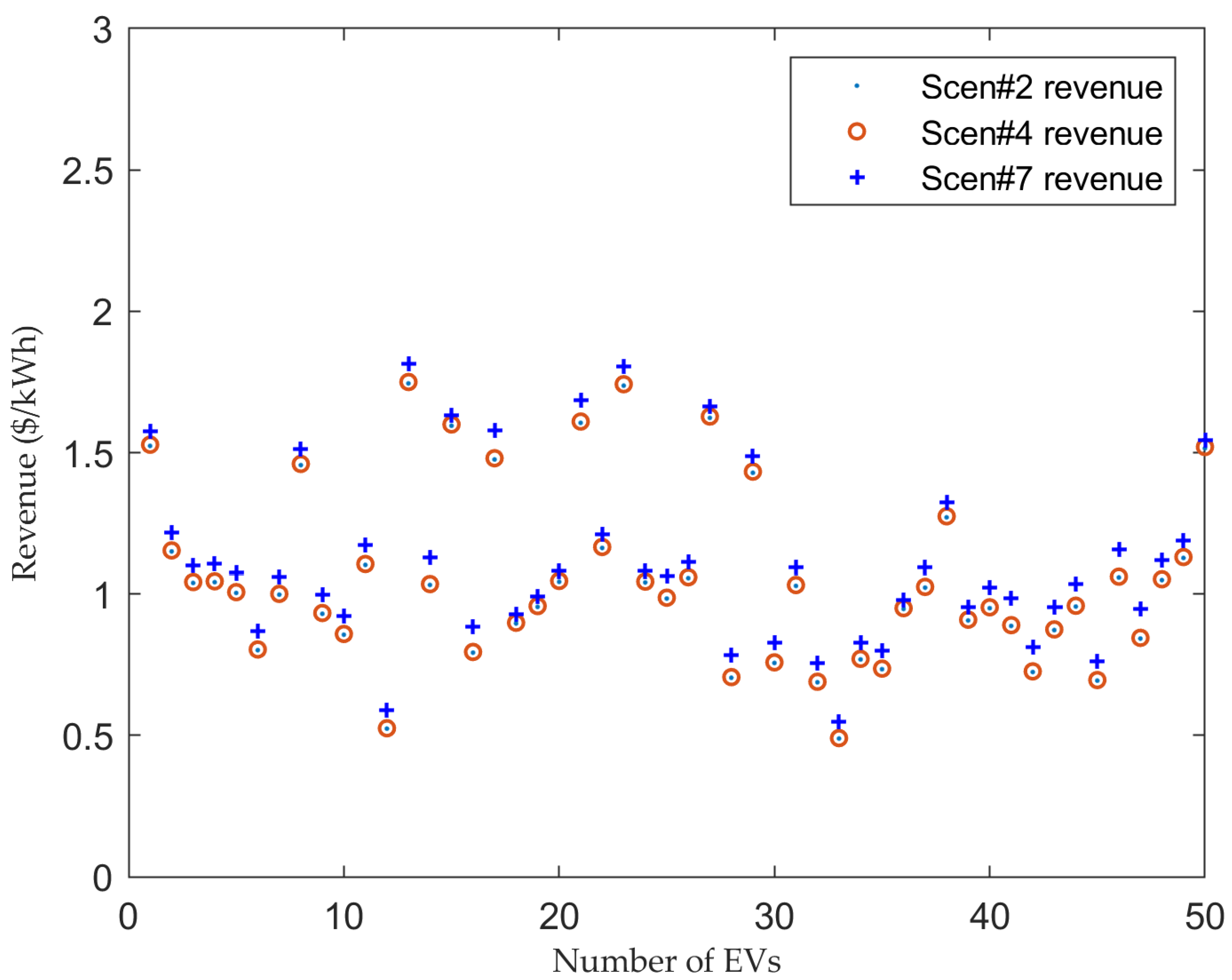
Figure 15 shows the revenue in the frequency regulation in Scenarios #2, #4 and #7. It shows the effect of incorporating the degradation cost to the objective function on increasing the revenue for each agent. The daily revenue for each agent fluctuates between USD 0.5 and USD 1.7.
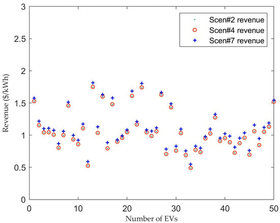
Figure 15.
Daily revenue for each vehicle.
In this study, the at the start of driving time ( and ) was set at 50%, which provides a sufficient amount of energy for driving.
4. Discussion
This study develops both centralized and distributed optimization models for s to participate in frequency regulation of power systems. Case studies were conducted in seven scenarios using real data to evaluate the proposed models. Table 2 summarizes the MAPE and MAE in Scenarios #2, #4, and #7. Table 3 summarizes the reward, degradation cost, charging cost, and revenue in Scenarios #2, #4, and #7, where .
Table 2.
MAPE and MAE values with and without considering the battery bank.
Table 3.
The reward, degradation cost, charging cost, and revenue.
As can be seen from Table 2, there is a mismatch between aggregated charging and discharging and the reference signal since the s are not available for frequency regulation during driving or the reaches its limit. This shows the importance of modeling the dynamic usages.
Both the centralized model (Scenario #2) and the distributed model (Scenario #4) show good performance in frequency regulation. Specifically, as can be seen from Table 2, the MAE of using the distributed model was 0.0067 kW. This performance is as good as the centralized model, in which the MAE is 0.014 kW. Furthermore, the total revenue in Scenario #4 is USD 52.75 compared with USD 52.59 in Scenario #2 as shown in Table 3.
However, owners may hesitate to share their private information such as the driving time, the driving periods, plug-in time, contracted rewards, and battery . Furthermore, owners want to have complete decision making over their s, and the centralized model takes this right away from them. This can lead to an unsuccessful V2G application. In the distributed approach, each owner obtains global information such as frequency regulation signals and the aggregated charging and discharging profile of the other s from the aggregator. Based on this information, the schedules its charging and discharging energy by solving the proposed distributed optimization model. Through the coordination of the aggregator, a global optimal solution can be reached. Because the s do not need to share their private information with the other owners, privacy is preserved.
In addition, the central failure problem represents a major defect of the centralized model. For Scenario #3, Figure 9 shows that when the central computer is down from 12:00 to 14:00, charging and discharging of all the vehicles are not under control. In other words, all vehicles become passive load and start to charge themselves, which increases the frequency deviation. In contrast, by using the distributed model, Scenario #6 shows that even with 10 out of 50 s failing in their commitment, the rest of the s could regulate the frequency without noticeable underperformance.
Another major problem of the centralized model is that the model complexity increases quickly when the number of s increases. In other words, powerful computers with large memory are needed to solve the centralized model for a large number of s. In contrast, the distributed model needs much less memory and computational power since each subproblem is much simpler than the centralized model. For example, the distributed model is solved with 500 s in Scenario #5. In addition, the computation time of using the distributed model in Scenario #4 was 21 s, while the computation time of the centralized model in Scenario #2 was 1815 s.
Frequent charging and discharging to provide frequency regulation services can reduce battery lifetime; therefore, the proposed model includes the battery degradation cost in the objective function. The performance was evaluated in Scenario #7. From Table 3, we can see that the reward is reduced from USD 262.57 in Scenario #4 to USD 255.8 in Scenario #7 due to less frequent charging and discharging. However, the degradation cost also decreases. In fact, the total revenue increases from USD 52.75 to USD 55.87, which shows the importance of incorporating the degradation cost into the objective function. This also shows that including degradation cost can make the model more accurate and useful.
In addition, V2G participation does not affect usage since a minimum accepted before the driving time is included in the models. Specifically, the right before driving is maintained greater than or equal to , which is sufficient for daily driving.
The obtained results show that the proposed models not only provide a frequency regulation service to the power system but also increase revenue to the owners without sacrificing privacy. Furthermore, the whole system saves more than USD 337.5 due to using s for frequency regulation. The system pays approximately USD 262.0 per day for s as a reward; otherwise, it would spend USD 599.5 in the electricity market for frequency regulation.
5. Conclusions
This study proposes both centralized and distributed optimal V2G models for frequency regulation. Dynamic usage patterns and battery degradation are modeled. By introducing three sets of variables (, , and ), undesired charging and discharging behavior is avoided. In addition, V2G problems are formulated as LP models, which can be solved efficiently by the embedded energy management system in s. Simulation results show that the centralized model can aggregate s to match the required regulation signals while owners can obtain rewards. The centralized model can be used by aggregators, utilities, and system operators to plan V2G applications. However, it may not be suitable for real-time implementation due to privacy concerns, high complexity, scalability limitation, and central failure issues. The proposed distributed V2G model can overcome these limitations and shows promising results. Simulation results also show that dynamic usage and battery degradation have significant impact on the V2G application and including them can improve the model accuracy. The proposed approaches can be used to turn the fleet s to an eco-friendly energy source for frequency regulation and to encourage owners to participate in V2G applications.
Author Contributions
Conceptualization, Z.W.; Formal analysis, M.E.-H.; Investigation, M.E.-H., X.L.; Methodology, M.E.-H., Z.W., X.L.; Software, M.E.-H., Z.W.; Supervision, Z.W.; Writing—original draft, M.E.-H.; Writing—review & editing, Z.W., X.L. All authors have read and agreed to the published version of the manuscript.
Funding
This work was funded in part by the Graduate Student Base Funding at the University of Regina and Mitacs Research Training Award (IT20451).
Conflicts of Interest
The authors declare no conflict of interest.
References
- Liu, H.; Huang, K.; Wang, N.; Qi, J.; Wu, Q.; Ma, S.; Li, C. Optimal dispatch for participation of electric vehicles in frequency regulation based on area control error and area regulation requirement. Appl. Energy 2019, 240, 46–55. [Google Scholar] [CrossRef]
- Hui, H.; Ding, Y.; Song, Y.; Rahman, S. Modeling and control of flexible loads for frequency regulation services considering compensation of communication latency and detection error. Appl. Energy 2019, 250, 161–174. [Google Scholar] [CrossRef]
- Yang, D.; Gao, H.C.; Zhang, L.; Zheng, T.; Hua, L.; Zhang, X. Short-term frequency support of a doubly-fed induction generator based on an adaptive power reference function. Int. J. Electr. Power Energy Syst. 2020, 119, 105955. [Google Scholar] [CrossRef]
- Delavari, A.; Kamwa, I. Improved optimal decentralized load modulation for power system primary frequency regulation. IEEE Trans. Power Syst. 2017, 33, 1013–1025. [Google Scholar] [CrossRef]
- Amamra, S.A.; Marco, J. Vehicle-to-Grid Aggregator to Support Power Grid and Reduce Electric Vehicle Charging Cost. IEEE Access 2019, 7, 178528–178538. [Google Scholar] [CrossRef]
- Erdogan, N.; Erden, F.; Kisacikoglu, M. A fast and efficient coordinated vehicle-to-grid discharging control scheme for peak shaving in power distribution system. J. Mod. Power Syst. Clean Energy 2018, 6, 555–566. [Google Scholar] [CrossRef] [Green Version]
- Huang, Y. Day-ahead optimal control of PEV battery storage devices taking into account the voltage regulation of the residential power grid. IEEE Trans. Power Syst. 2019, 34, 4154–4167. [Google Scholar] [CrossRef]
- Ko, K.S.; Han, S.; Sung, D.K. Performance-based settlement of frequency regulation for electric vehicle aggregators. IEEE Trans. Smart Grid 2016, 9, 866–875. [Google Scholar] [CrossRef]
- Farzin, H.; Fotuhi-Firuzabad, M.; Moeini-Aghtaie, M. Reliability studies of modern distribution systems integrated with renewable generation and parking lots. IEEE Trans. Sustain. Energy 2016, 8, 431–440. [Google Scholar] [CrossRef]
- Singh, S.; Pamshetti, V.B.; Singh, S. Time Horizon-Based Model Predictive Volt/VAR Optimization for Smart Grid Enabled CVR in the Presence of Electric Vehicle Charging Loads. IEEE Trans. Ind. Appl. 2019, 55, 5502–5513. [Google Scholar] [CrossRef]
- Sabhahit, J.N.; Solanke, S.S.; Jadoun, V.K.; Malik, H.; García Márquez, F.P.; Pinar-Pérez, J.M. Contingency Analysis of a Grid of Connected EVs for Primary Frequency Control of an Industrial Microgrid Using Efficient Control Scheme. Energies 2022, 15, 3102. [Google Scholar] [CrossRef]
- Lam, A.Y.; Leung, K.C.; Li, V.O. Capacity estimation for vehicle-to-grid frequency regulation services with smart charging mechanism. IEEE Trans. Smart Grid 2015, 7, 156–166. [Google Scholar] [CrossRef] [Green Version]
- Aziz, M.; Huda, M. Utilization of electric vehicles for frequency regulation in Danish electrical grid. Energy Procedia 2019, 158, 3020–3025. [Google Scholar] [CrossRef]
- Han, S.; Han, S.; Sezaki, K. Development of an optimal vehicle-to-grid aggregator for frequency regulation. IEEE Trans. Smart Grid 2010, 1, 65–72. [Google Scholar]
- Ginigeme, K.; Wang, Z. Distributed Optimal Vehicle-To-Grid Approaches With Consideration of Battery Degradation Cost Under Real-Time Pricing. IEEE Access 2020, 8, 5225–5235. [Google Scholar] [CrossRef]
- Iqbal, S.; Xin, A.; Jan, M.U.; ur Rehman, H.; Masood, A.; Rizvi, S.A.A.; Salman, S. Aggregated Electric Vehicle-to-Grid for Primary Frequency Control in a Microgrid-A Review. In Proceedings of the 2018 IEEE 2nd International Electrical and Energy Conference (CIEEC), Beijing, China, 4–6 November 2018; pp. 563–568. [Google Scholar]
- Tan, J.; Wang, L. A game-theoretic framework for vehicle-to-grid frequency regulation considering smart charging mechanism. IEEE Trans. Smart Grid 2016, 8, 2358–2369. [Google Scholar] [CrossRef]
- Escudero-Garzás, J.J.; García-Armada, A.; Seco-Granados, G. Fair design of plug-in electric vehicles aggregator for V2G regulation. IEEE Trans. Veh. Technol. 2012, 61, 3406–3419. [Google Scholar] [CrossRef] [Green Version]
- Faddel, S.; Aldeek, A.; Al-Awami, A.T.; Sortomme, E.; Al-Hamouz, Z. Ancillary services bidding for uncertain bidirectional V2G using fuzzy linear programming. Energy 2018, 160, 986–995. [Google Scholar] [CrossRef]
- Sortomme, E.; El-Sharkawi, M.A. Optimal charging strategies for unidirectional vehicle-to-grid. IEEE Trans. Smart Grid 2010, 2, 131–138. [Google Scholar] [CrossRef]
- Ahn, C.; Li, C.T.; Peng, H. Optimal decentralized charging control algorithm for electrified vehicles connected to smart grid. J. Power Sources 2011, 196, 10369–10379. [Google Scholar] [CrossRef]
- Shuai, W.; Maillé, P.; Pelov, A. Charging electric vehicles in the smart city: A survey of economy-driven approaches. IEEE Trans. Intell. Transp. Syst. 2016, 17, 2089–2106. [Google Scholar] [CrossRef] [Green Version]
- Mu, Y.; Wu, J.; Ekanayake, J.; Jenkins, N.; Jia, H. Primary frequency response from electric vehicles in the Great Britain power system. IEEE Trans. Smart Grid 2012, 4, 1142–1150. [Google Scholar] [CrossRef]
- Liu, H.; Qi, J.; Wang, J.; Li, P.; Li, C.; Wei, H. EV dispatch control for supplementary frequency regulation considering the expectation of EV owners. IEEE Trans. Smart Grid 2016, 9, 3763–3772. [Google Scholar] [CrossRef] [Green Version]
- Vachirasricirikul, S.; Ngamroo, I. Robust LFC in a smart grid with wind power penetration by coordinated V2G control and frequency controller. IEEE Trans. Smart Grid 2014, 5, 371–380. [Google Scholar] [CrossRef]
- Wang, X.; He, Z.Y.; Yang, J.W. Unified strategy for electric vehicles participate in voltage and frequency regulation with active power in city grid. IET Gener. Transm. Distrib. 2019, 13, 3281–3291. [Google Scholar] [CrossRef]
- Jin, C.; Li, W.; Shen, J.; Li, P.; Liu, L.; Wen, K. Active frequency response based on model predictive control for bulk power system. IEEE Trans. Power Syst. 2019, 34, 3002–3013. [Google Scholar] [CrossRef]
- Peng, C.; Zou, J.; Lian, L.; Li, L. An optimal dispatching strategy for V2G aggregator participating in supplementary frequency regulation considering EV driving demand and aggregator’s benefits. Appl. Energy 2017, 190, 591–599. [Google Scholar] [CrossRef]
- El-Hendawi, M.; Wang, Z. Multi-agent Optimization for Frequency Regulation through Vehicle-to-Grid Applications. In Proceedings of the IEEE 92nd Vehicular Technology Conference, Victoria, BC, Canada, 18 November–16 December 2020; pp. 1–5. [Google Scholar]
- Molzahn, D.K.; Dörfler, F.; Sandberg, H.; Low, S.H.; Chakrabarti, S.; Baldick, R.; Lavaei, J. A survey of distributed optimization and control algorithms for electric power systems. IEEE Trans. Smart Grid 2017, 8, 2941–2962. [Google Scholar] [CrossRef]
- Yang, J.; Feng, W.; Hou, X.; Xia, Q.; Zhang, X.; Wang, P. A Distributed Cooperative Control Algorithm for Optimal Power Flow and Voltage Regulation in DC Power System. IEEE Trans. Power Deliv. 2019, 35, 892–903. [Google Scholar] [CrossRef]
- Hao, R.; Lu, T.; Wu, Q.; Chen, X.; Ai, Q. Distributed Piecewise Approximation Economic Dispatch for Regional Power Systems Under Non-Ideal Communication. IEEE Access 2019, 7, 45533–45543. [Google Scholar] [CrossRef]
- Du, P.; Ran, L.; Zhai, D.; Ren, R.; Zeng, Q. ADMM-Based Distributed Online Algorithm for Energy Management in Hybrid Energy Powered Cellular Networks. IEEE Access 2019, 7, 83343–83353. [Google Scholar] [CrossRef]
- Wu, Z.; Chen, B. Distributed Electric Vehicle Charging Scheduling with Transactive Energy Management. Energies 2021, 15, 163. [Google Scholar] [CrossRef]
- Wang, Z.; Paranjape, R. Optimal residential demand response for multiple heterogeneous homes with real-time price prediction in a multiagent framework. IEEE Trans. Smart Grid 2015, 8, 1173–1184. [Google Scholar] [CrossRef]
- Ontario’s Independent Electricity System Operator (IESO). Available online: http://www.ieso.ca (accessed on 1 March 2022).
- Lu, J.; Hossain, J. Vehicle-to-Grid: Linking Electric Vehicles to the Smart Grid; IET Power and Energy Series; Institution of Engineering and Technology: Stevenage, UK, 2015; Volume 79. [Google Scholar]
- David, A.O.; Al-Anbagi, I. EVs for frequency regulation: Cost benefit analysis in a smart grid environment. IET Electr. Syst. Transp. 2017, 7, 310–317. [Google Scholar] [CrossRef]
- Xu, B.; Oudalov, A.; Ulbig, A.; Andersson, G.; Kirschen, D.S. Modeling of lithium-ion battery degradation for cell life assessment. IEEE Trans. Smart Grid 2016, 9, 1131–1140. [Google Scholar] [CrossRef]
- Boyd, S.; Parikh, N.; Chu, E.; Peleato, B.; Eckstein, J. Distributed optimization and statistical learning via the alternating direction method of multipliers. Found. Trends Mach. Learn. 2011, 3, 1–122. [Google Scholar]
- Journey to Work: Key Results from the 2016 Census. Available online: https://www150.statcan.gc.ca/n1/dailyquotidien/171129/dq171129c-eng.htm (accessed on 1 November 2021).
- Commuting in Canada: How Your Drive to Work Stacks Up. Available online: https://www.insurancehotline.com/resources/commuting-in-canada-howyour-drive-to-work-stacks-up-infographic/ (accessed on 1 November 2021).
- Daily EV Energy Consumption for Driving. Available online: https://www.virta.global/blog/ev-charging-101-how-much-electricity-does-an-electric-car-use (accessed on 1 November 2021).
- Ancillary Service Market Price. Available online: http://dataminer2.pjm.com/feed/reserve-market-results (accessed on 5 May 2021).
- Saskpower Residential Power Rates. Available online: https://www.saskpower.com/Accounts-and-Services/Billing/Power-Rates/Power-Supply-Rates (accessed on 6 September 2021).
- Kolawole, O.; Al-Anbagi, I. Electric vehicles battery wear cost optimization for frequency regulation support. IEEE Access 2019, 7, 130388–130398. [Google Scholar] [CrossRef]
- Grant, M.; Boyd, S. CVX: Matlab Software for Disciplined Convex Programming, Version 2.1. 2014. Available online: http://cvxr.com/cvx (accessed on 10 October 2021).
- ApS, M. Mosek optimization toolbox for matlab. In User’s Guide and Reference Manual; Version 4; MOSEK: Copenhagen, Denmark, 2019. [Google Scholar]
- Grant, M.; Boyd, S. Graph implementations for nonsmooth convex programs. In Recent Advances in Learning and Control; Blondel, V., Boyd, S., Kimura, H., Eds.; Lecture Notes in Control and Information Sciences; Springer: London, UK, 2008; pp. 95–110. [Google Scholar]
- Wang, Z.; Zhong, J.; Li, J. Design of performance-based frequency regulation market and its implementations in real-time operation. Int. J. Electr. Power Energy Syst. 2017, 87, 187–197. [Google Scholar] [CrossRef]
- El-Hendawi, M.; Wang, Z. An ensemble method of full wavelet packet transform and neural network for short term electrical load forecasting. Electr. Power Syst. Res. 2020, 182, 106265. [Google Scholar] [CrossRef]
- Brooks, A.E.; Lesieutre, B.C. RTO Frequency Regulation Market Clearing Formulations and the Effect of Opportunity Costs on Electricity Prices. arXiv 2020, arXiv:2001.11134. [Google Scholar]


Publisher’s Note: MDPI stays neutral with regard to jurisdictional claims in published maps and institutional affiliations. |
© 2022 by the authors. Licensee MDPI, Basel, Switzerland. This article is an open access article distributed under the terms and conditions of the Creative Commons Attribution (CC BY) license (https://creativecommons.org/licenses/by/4.0/).