A Non-Invasive Method Based on AI and Current Measurements for the Detection of Faults in Three-Phase Motors

Abstract

Three-phase motors are commonly adopted in several industrial contexts and their failures can result in costly downtime causing undesired service outages; therefore, motor diagnostics is an issue that assumes great importance. To prevent their failures and face the considered service outages in a timely manner, a non-invasive method to identify electrical and mechanical faults in three-phase asynchronous electric motors is proposed in the paper. In particular, a measurement strategy along with a machine learning algorithm based on an artificial neural network is exploited to properly classify failures. In particular, digitized current samples of each motor phase are first processed by means of FFT and PSD in order to estimate the associated spectrum. Suitable features (in terms of frequency and amplitude of the spectral components) are then singled out to either train or feed a neural network acting as a classifier. The method is preliminarily validated on a set of 28 electric motors, and its performance is compared with common state-of-the-art machine learning techniques. The obtained results show that the proposed methodology is able to reach accuracy levels greater than 98% in identifying anomalous conditions of three-phase asynchronous motors.

1. Introduction

The three-phase asynchronous motor is widely used as an electric drive thanks to its design simplicity, low production cost, sturdiness and reliability. Furthermore, the asynchronous motor is characterized by a high efficiency. It can also be simply connected directly to the distribution network with constant voltage and frequency if it is not necessary to control its speed with an inverter. Induction motors are employed in various industries and often operate under harsh conditions. Thus, induction motors’ internal parts (such as stator, rotor insulation materials and bearings) can develop faults. Three-phase electric motors are devices that can therefore show failures due to mechanical and electrical faults [1,2]. Induction motors play an important role in industrial manufacturing. To get a sense of the impact of induction motors in the industrial field, it is worth noting that these devices account for 29% of global and 69% of industrial electricity consumption [3]. There is a growing need for online monitoring of the health of systems to achieve the high standards of safety and reliability that many industrial contexts require [4]. Efficient diagnostic procedures help to maintain high levels of reliability, availability, maintainability and safety (RAMS) of the monitored systems [5]. The operating conditions of the motors typically prevent adequate modeling from an analytical approach, as it would be necessary to take into account model issues such as workloads, ambient noise and transient depending on the specific environments and system these motors are exploited in [6]. Therefore, multiple solutions based on machine learning are emerging in order to meet the diagnostic needs of the mechanical components that make up devices commonly adopted in industrial contexts [7,8]. Recent advancements in signal processing and artificial intelligence have attracted renewed interest in induction motor diagnostics, thus model-based approaches can be replaced thanks to the machine learning-based fault diagnosis methods [9]. Induction motor faults are mainly diagnosed by using characteristic signals of the motors, such as vibration signals, thermal images, acoustic signals and motor currents [10]. Unfortunately, most techniques require system modifications (i.e., sensor installation) or complete observation (such as for fault monitoring through infrared sensors). On the contrary, investigating diagnostic solutions useful for those production contexts in which the motors could be inaccessible for the application of diagnostic sensors and the only measurable physical quantities are those associated with motor power supply is advisable. A promising technique for diagnostics is based on the stator current analysis which has been demonstrated to be useful for preventing catastrophic motor failures caused by inter-turn short circuit faults in permanent magnet wind generators [11].

In this paper, the issue of motor diagnostics is addressed by means of machine learning and preprocessing techniques applied to current measurements collected from the motor power supply. The proposed method is based on the acquisition of samples of the motor current signals and the use of machine learning techniques based on artificial neural networks for the classification of the motor health status. More specifically, the proposed solution is designed to be implemented in edge computing solutions; to this aim, both techniques of feature extractions and machine learning algorithms have to be as lightweight as possible to be integrated into embedded solutions. Moreover, the non-invasiveness and the high efficacy constitute the novelty of this work; finally, the method performance has been assessed, according to the authors’ best knowledge, on the largest dataset of three-phase motors ever presented as the state of the art.

The paper is organized as follows: in Section 2 a state-of-the-art overview is reported and recent improvements’ limits are discussed; an overview of artificial neural network fundamentals is shown in Section 3; Section 4 presents the proposed method for a non-invasive fault detection based on current measurements and AI algorithms; Section 5 introduces a case study of 28 electrical motors; in Section 5.3, a comparison between the proposed AI algorithms and the most common AI algorithms in predictive maintenance is reported. Conclusions and final remarks are highlighted in Section 6.

2. Related Works in Diagnostics for Induction Motors

The progress achieved in the field of motor diagnostics and machine learning techniques is evident in the current state of the art. In recent years, diagnostics of electric motors and health monitoring techniques have become a task of great relevance, as timely maintenance through early detection of irregularities during the normal machine operation can be achieved [12]. Due to the importance of this field, many methods have emerged to carry out diagnostics and predictive maintenance.

New machine learning techniques for prediction tasks are proposed as the state of the art, such as the non-iterative supervised learning predictors based on Ito decomposition and the structure successive geometric transformations model or the convolutional and long short-term memory neural networks, generally used for other purposes such as image processing and classification [13,14,15,16,17].

Lingxin Li and Chris Mechefske in [18] report statistics about failure causes. About 50% of failures are caused by bearing failures, around 40% are due to winding failures of the stator and the remaining 10% are due to failures of the rotor or the shafts.

An interesting method for online diagnostics has been presented in [19] where the authors proposed the measurement of the frequency response in motor windings in order to perform detection of both mechanical and electrical damage (i.e., deformation of the windings and degradation of conductors and materials for isolation). This method is very interesting as it can be easily integrated into systems based on asynchronous motors and allows for real-time diagnostics. The fact that it does not interfere with normal motor operations is its main strength. Unfortunately, the method requires a thorough knowledge of the type of motor being observed and, consequently, the methodology is difficult to implement on a large scale. Furthermore, the authors do not introduce a quantitative measure of the real ability of the method to identify failures. Finally, the case studies are limited to simulated and not actual faults so there are not enough data to suggest a real applicability.

The methodology proposed in [20] addresses the problem of rotor manufacturing inaccuracies caused during the die casting process. Depending on the importance, this type of problem can present itself immediately or remain hidden until it manifests itself in critical moments of the use of motors. However, this method can only be used offline and is invasive as it is necessary to disassemble the motor.

A smart-sensor has been proposed in [12]; it is based on low-cost compact triaxial stray flux sensors whose setup is easy and non-invasive. Despite these advantages, sensors need to be applied to specific locations on the motors and, consequently, an offline and invasive intervention on the motor needs to be performed.

An interesting comparison between vibrations and current monitoring is presented in [21]. The authors pointed out that methods based on current and vibration analysis are the most widely used techniques for motor diagnostics. This is explained by the advantages of reliability, non-invasiveness and ease of installation of the measuring sensors. The authors applied the support vector machine algorithm to the different cases of failures and measured signals. With the support vector machine it is shown that mechanical failures are better identified by means of vibration signals and electrical failures are well identified by current measurements. It is also pointed out that the accuracy of the diagnostics varies according to the motor speed. Although it is possible to achieve satisfactory accuracy in some contexts, a valid method is not proposed to diagnose every type of fault by means of current signals alone. Furthermore, the authors do not propose a method for the choice of measurement and diagnostic instruments. Finally, the applied method does not seem to be applicable in real time on an embedded device but rather requires an offline computer analysis.

A graph-based semi-supervised learning has been proposed in [9] in order to develop a comprehensive fault diagnosis method for online diagnostics on induction motors. The proposed method is an approach based on semi-supervised learning which requires a smaller amount of labeled data; in particular, the authors adopted the greedy-gradient max cut algorithm (GGMC). The authors noted that a large labeled dataset is required for supervised machine learning methods, which is not always available in real operating conditions. The method responds to the need to have a consistent training dataset. However, the proposed method has been validated on the same motors used for training, although the data on which the approach has been validated are not the same. Thus, there is no information on the validity of the approach in a real context. Finally, the authors do not specify the system requirements to be able to build a diagnostic system for a large-scale application.

3. Fundamentals of Feed-Forward Neural Network

The machine learning technologies adopted in this paper have been appropriately selected for their simplicity, thus making their implementation in embedded solutions and execution in microcontrollers possible. The proposed method exploits a feed-forward artificial neural network (ANN) as a machine learning model. The feed-forward ANN’s connections between the units do not form cycles. In the case of feed-forward networks, the function in Equation (2) is transformed consequently and it is necessary to introduce the concept of neurons (hence the name) to explain it.

Given an input vector I, a neuron consists of an activation function $\varphi$ that takes as input the weighted sum of the elements of the vector I (Figure 1). This simple neuron is called a perceptron, introduced by Rosenblatt in 1962. Usually, a threshold is included in the neuron model, adding a fictitious input with a value fixed at 1, and the weight of the connection is given by $-t$ that can be imagined as an additional neuron with no input values. Formally, the function of the neuron becomes:

$$O=\varphi (\sum _{i=0}^n{\omega }_i{I}_i)$$

(1)

where n is the total number of the neuron’s inputs.

The activation function $\varphi$ can be of different types, and the ones that are adopted in this proposed methodology are listed below.

• Rectified linear unit (ReLU) which is an activation function defined as the positive part of its argument (Figure 2a), the function $\varphi$ is $\varphi \left(x\right)=max(0,x)$;
• hyperbolic tangent (Tanh) which is an activation function defined as $tanh\left(x\right)$ (Figure 2b), thus the function $\varphi$ becomes $\varphi \left(x\right)=\frac{e^x-e^{-x}}{e^x+e^{-x}}$;
• sigmoid, sometimes named as logistic or soft step (Figure 2c), whose function is $\varphi \left(x\right)=\frac{1}{1+e^{-x}}$.

Figure 2. Activation functions. (a) ReLU. (b) Tanh. (c) Sigmoid.

Figure 2. Activation functions. (a) ReLU. (b) Tanh. (c) Sigmoid.

It is important to note that in the configuration of the neural network architecture, the activation function is a very important hyperparameter in order to achieve high performance. All neurons therefore contribute to form the network. If the output of a neuron is linked in input to a new neuron, the latter contributes to form a level that is defined as a deep level. Hence, the network is organized in levels: each neuron of a level receives input only from the neurons of the previous level; it propagates the outputs only towards the neurons of the following levels. The layers between the inputs and the output are called hidden layers. Self-connections are not allowed in this type of network, nor are connections between neurons belonging to the same level. Each neuron, therefore, has the function of propagating the signal through the network, with a flow of information that goes from the previous level to the next level (the levels could coincide with the input or output of the network). It follows that the first level of the neural networks takes the argument of Equation (3) as input.

In Figure 3, a generic architecture of a feed-forward neural network is reported, where $l\in \{2,\dots ,L\}$ is the layer index, the total number of hidden levels is L and $A_l$ is the generic number of neurons per level l. The number of intermediate levels ($L-1$), the number of neurons for each level ($A_l$) and the activation functions ($\varphi \left(x\right)$) are hyperparameters that compose the architecture configuration and should be established at the first stage, in order to obtain the topology, the number and type of neurons, the connections, etc. Further hyperparameters are added that do not describe the architecture in the strict sense but contribute to the performance of the model: regularization strength (Lambda) and the standardize data option. The regularization strength (Lambda) hyperparameter specifies the regularization penalty term and the standardize data binary hyperparameter specifies whether to standardize the numeric predictors or not, in the case of predictors with widely different scales. The term of the regularization penalty affects the weight of the regularization; in particular, the risk of overfitting is prevented or increased according to the regularization value.

Once the architecture is ready, the second stage is to determine the weights of the connections in order to build a classifier, based on the training dataset made available to the network (placed in input), this phase is named training.

4. Proposed Method

Therefore, the issue of performing fault detection must be addressed by adopting a classifier that, on the one hand, ensures a satisfactory level of accuracy in the prediction of failures and, on the other hand, allows the diagnostic system to be easily integrated into edge computing solutions.

The goal is therefore to train an algorithm represented by a function $f\left(X\right)$ that, given the current signals measured on the power supply line, returns a symbol that identifies the class to which the signals belong (healthy/broken). The function to be constructed is therefore a relationship between a set of cardinality m to a set of cardinality 1. The function $f\left(X\right)$ is therefore the following:

$$Y=f\left(X\right):R^m\to R^1$$

(2)

where m is the number of features and $R^1$ is the label set. The function, therefore, represent the classification algorithm and the output is the result of the classification.

The features extracted from the signal are derived from the spectral analysis of the acquired current signals. The method proposed in this paper does not use time domain features in order to keep the algorithms independent of the time of observation of the signals. Naturally, a longer observation time of the signal allows a higher quality of the samples thanks to the consequent reduction in the noise floor. The method is mainly based on fast Fourier transform (FFT) and power spectral density (PSD) components as they are easily computable components in embedded solutions such as microcontrollers or digital signal processors (DSPs) for which libraries and dedicated hardware are generally available. In particular, the largest spectral components of the FFT and the largest components of the PSD are collected from each signal. For each component, amplitude–frequency pairs are selected. The method proposed hereinafter adopts both FFT and PSD because the aim is to extract a set of characteristics from the signals that are representative of the failure phenomena but synthetic to avoid an excessive amount of information in the signals causing risks of overfitting. A failure cannot be identified on the basis of thresholds in the FFT or PSD components alone. This is the reason why the proposed method adopts a more complex inferential modeling with a fixed number of features extracted from both the FFT and the PSD.

According to the considered inputs, the function of the classifier therefore becomes:

$$Y=f({\mathit{F}}^{FFT},{\mathit{A}}^{FFT},{\mathit{F}}^{PSD},{\mathit{A}}^{PSD}),$$

(3)

where $\mathit{F}$ and $\mathit{A}$ represent frequencies and amplitudes, respectively. The number of components to be selected must be large enough to represent the reconstructed signal with suitable approximation. At the same time, it is not advisable to select too large a number of components for reasons of computational complexity and overfitting problems. It should be noted that an excessive number of components (FFT and PSD) risks being representative not only of the useful signal but also of the measurement noise; moreover, a large number of features could reduce the model’s ability to recognize the same phenomena in typical signals of different motors.

The model therefore takes as input the features described above extracted from the observations collected from the supply line.

Figure 4 summarizes the method proposed in this paper. A data acquisition unit (DAQ) collects samples from the three-phase motor power supply currents. Metrological characteristics of the DAQ have to be accurately selected in terms of both memory depth and sampling rate to accomplish the desired task. Acquired samples are then processed in order to achieve the associated spectral components of interest. Finally, the features are extracted in order to make them suitable for ANN training. This process differs in production from the last stage. The trained ANN model is used as classifier and the result represents the electrical motor health state.

However, the choice of the hyperparameters that describe the architecture must be guided by a technical approach because the number and the value of hyperparameter combinations can be huge. Of course, the goal is to maximize the classifier performances while trying to minimize the complexity of the architecture.

The hyperparameter configuration can be chosen via a grid search-based approach, which consists of an exhaustive search in a limited range of possible configurations, or by a random search-based approach, which consists of a non-exhaustive and random search for configurations in a range of possible combinations. In the case of large number of hyperparameters, the random search technique is to be preferred over the grid search from the point of view of computational times, because it has been demonstrated that random search is able to preserve good performance [22].

5. Preliminary Performance Assessment

The case study on which the method was validated includes a set of motors of various natures and different working conditions.

5.1. Measurement Setup

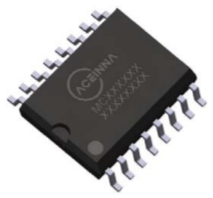
To assess the performance of the methods, a proper measurement station based on an embedded platform has been designed and implemented. In particular, the current sensor chosen for the acquisition is the MCR1101-20-5 (Figure 5). The main sensor specifications are reported in

Table 1. MCR 1101-20-5 sensor’s characteristics.

Parameter	Typical Value for $\mathit{VCC}=5$ V and ${\mathit{T}}_{\mathit{A}}=25{}^{°}$C
Input Range	$\pm 20$ A
Sensitivity	100 mV/A
Zero Current Offset	$\pm 20$ mA
Sensitivity Error	$\pm 0.3\%$
Linearity Error	$\pm 0.3\% Full Scale$
Total Error	$\pm 0.6\% Reading$
Zero Current Offset Drift	$\pm 60$ mA
Sensitivity Drift	$\pm 0.3\%$
Total Error Drift	$\pm 0.4\% Full Scale$

.

It was decided to adopt this sensor due to its full-scale, passband and limited magnetic hysteresis characteristics. The sensor performance has been assessed in laboratory tests using the Fluke 5720A [23] calibrator and 5725A amplifier [24] as reference current sources. The evaluation of the magnetic hysteresis was performed by stimulating the sensor with increasing and decreasing current flows and acquiring ten thousand samples for each current step.

Obtained results are presented in

Table 2. Result of the test for the measurement hysteresis assessment.

${\mathit{I}}_{\mathit{nom}}\left[\mathit{A}\right]$	${\mathit{I}}_{\mathit{meas}}^{+}\left[\mathit{A}\right]$	${\mathit{\sigma }}^{+}$	${\mathit{I}}_{\mathit{meas}}^{-}$	${\mathit{\sigma }}^{-}$	$\mathbf{\Delta }$
−10.000	−9.872	0.007	−9.879	0.007	0.007
−9.000	−8.878	0.005	−8.889	0.007	−0.011
−8.000	−7.886	0.006	−7.901	0.006	−0.015
−7.000	−6.926	0.007	−6.911	0.006	0.015
−6.000	−5.913	0.008	−5.912	0.007	0.001
−5.000	−4.926	0.007	−4.942	0.007	−0.016
−4.000	−3.939	0.007	−3.940	0.007	−0.001
−3.000	−2.954	0.007	−2.953	0.007	0.001
−2.000	−1.972	0.008	−1.983	0.008	−0.011
−1.000	−0.978	0.007	−0.980	0.008	−0.002
0.000	0.010	0.008	0.009	0.008	−0.001
1.000	1.009	0.008	1.010	0.007	0.001
2.000	1.990	0.008	2.009	0.007	0.019
3.000	2.988	0.007	3.007	0.008	0.025
4.000	3.986	0.006	3.983	0.007	0.003
5.000	4.992	0.006	4.974	0.007	−0.018
6.000	5.982	0.006	5.970	0.007	−0.012
7.000	6.984	0.005	6.993	0.007	0.009
8.000	7.983	0.006	7.973	0.006	−0.010
9.000	8.961	0.006	8.957	0.006	−0.004
10.000	9.990	0.007	9.990	0.007	0.000

; for each value of nominal current $I_{n}om$, the averages of 10,000 samples for increasing ($I_{meas}^{+}$) and decreasing ($I_{meas}^{-}$) current flows as well as the respective standard deviation (${\sigma }^{+}$ and ${\sigma }^{-}$) are reported.

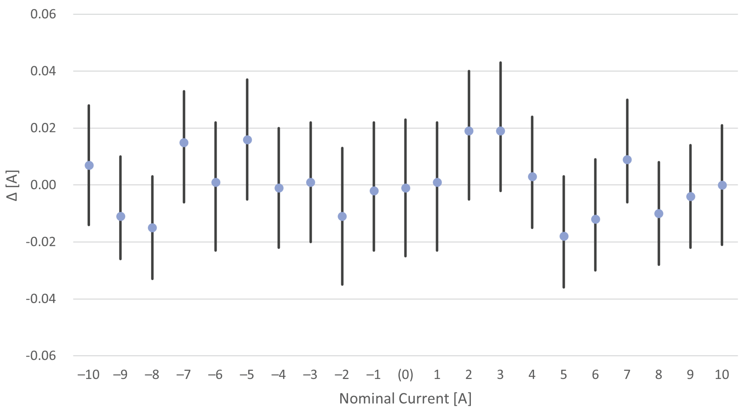
To better appreciate the sensor performance, the difference $\mathsf{\Delta }$ between increasing and decreasing currents has been provided.

Results are also summarized in Figure 6, where the evaluation of the differences $\mathsf{\Delta }$ versus the nominal currents is shown. Intervals centered in the difference $\mathsf{\Delta }$, whose half-amplitude is equal to three times the associated standard deviation, are also reported. As can be noticed, all the intervals are metrologically compatible with 0, thus ensuring a negligible contribution of the magnetic hysteresis in the considered application.

Gain and offset error, equal to $-0.838\%$ and 0.290 A, respectively, were also evaluated and compensated in the successive processing step.

The microcontroller (MCU) chosen for the measurement setup is the STM32F4V11VET. The MCU’s characteristics are written below and, for the sake of brevity, just information relevant for the case study are reported.

• Arm^® 32-bit Cortex^®-M4 CPU with FPU;
• 512 Kbytes of flash memory;
• 128 Kbytes of SRAM;
• general-purpose DMA;
• up to 11 timers;
• a 12-bit A/D converter 2.4 MSPS with 16 channels;
• up to 3 USARTs.

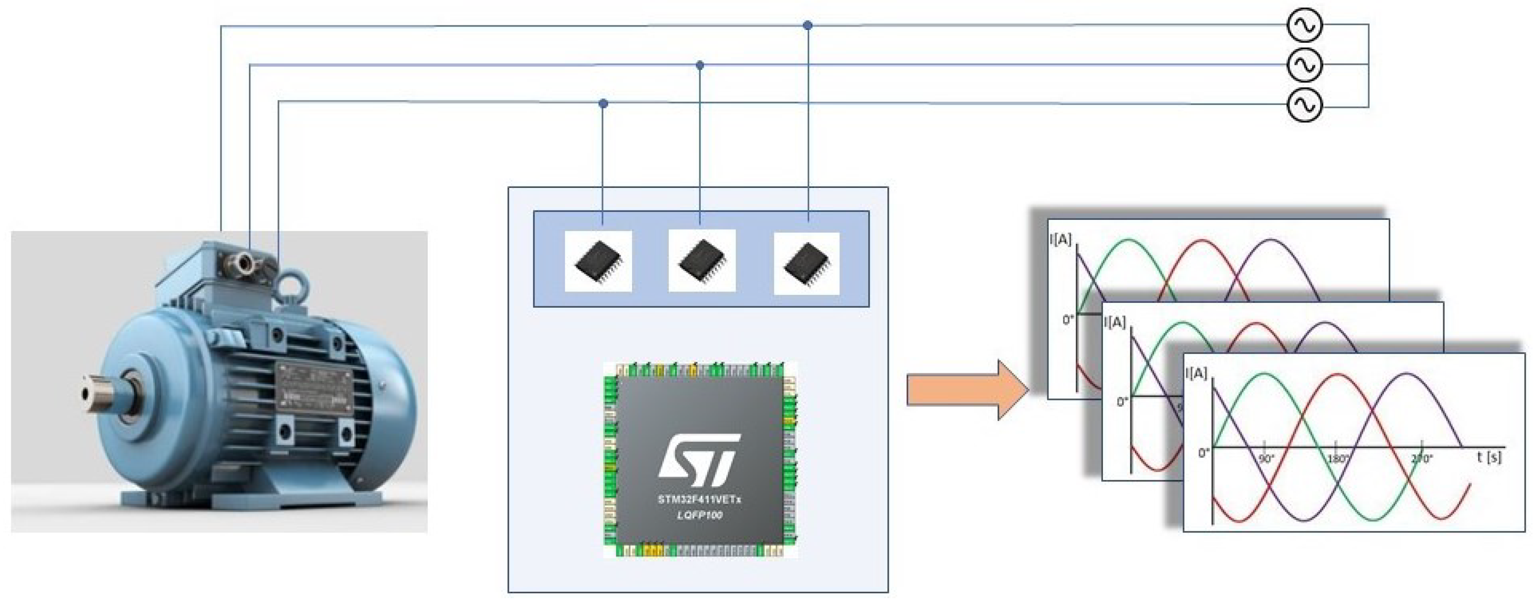
The current sensors output a voltage proportional to the measured current. Since it is necessary to acquire samples coming from 3 motor phases, 3 ADC channels have been used into which the voltage signals coming from the MCR1101-20-5 sensors are input (Figure 7).

It is necessary to reach a sampling rate in order to collect from the three channels measurements at 10,000 samples per second. This is possible by using the DMA and setting it so that as soon as the ADC produces a valid value, the DMA takes it to a buffer in RAM. Of course, it is necessary to reach a trade-off between sample size and available RAM resources.

In this case study, it was possible to acquire 20 whole periods with 20,000 samples for each phase, for a total buffer of 60,000 samples.

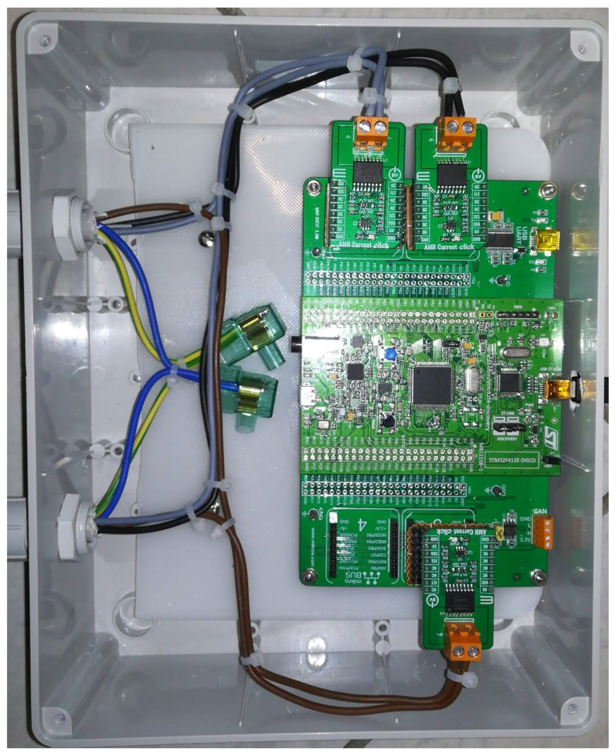
The device including sensors and wiring to operate the acquisitions is shown in Figure 8.

5.2. Feature Extraction and Modeling

To operate the measurement campaign, it was necessary to acquire samples from a large number of motors in different health conditions. Samples from the 3 power supply streams were collected for each motor. The dataset used for the case study is shown in

Table 3. Dataset exploited for the cross validation.

Classes	Number of Motors	Class Dimension
Healthy	7	21
Faulty	21	63

.

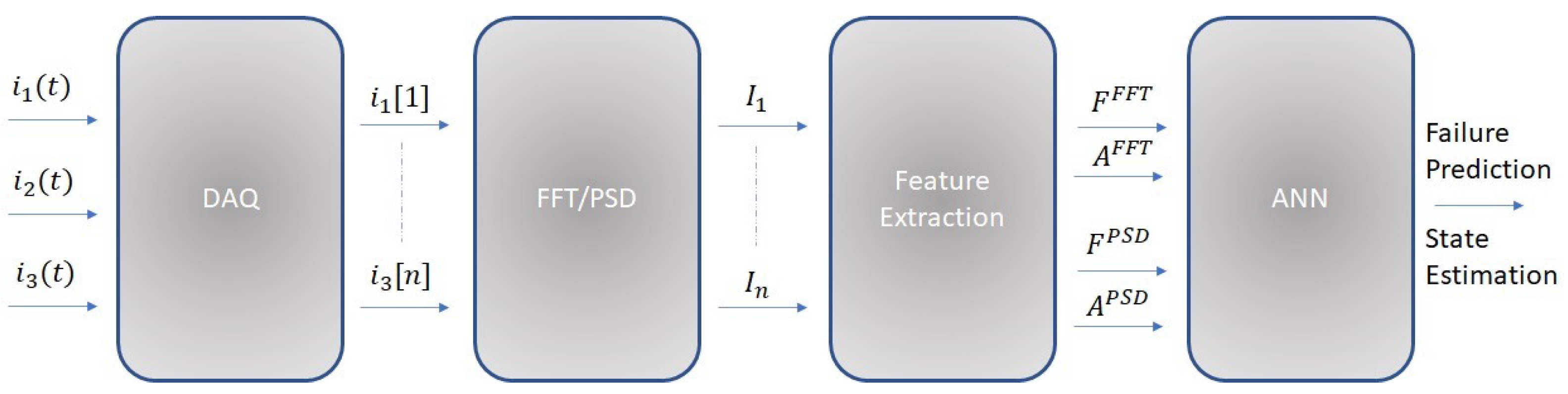
A large number of spectral components would allow having a complete description of the acquired signal but it would increase the consumption of computing and memory resources for the following steps. A trade-off between the dataset quality and the consumed hardware resources is required.

For each sample, the 10 largest frequency components of the fast Fourier transform (FFT) and the 10 largest components of the power spectral density (PSD) were selected.

The dataset is then created by taking the frequencies and amplitudes of the largest 10 components of the FFT and PSD.

$$\mathit{X}=\{f_1,A_1^{FFT},f_2,A_2^{FFT},\dots ,f_{10},A_{10}^{FFT},f_1,A_1^{PSD},f_2,A_2^{PSD},\dots ,f_{10},A_{10}^{PSD}\}.$$

(4)

The dataset is therefore composed of 40 features that describe, in a synthetic way and with a good approximation, the nature of the acquired signal. For the training and testing of the model, the k-fold technique was adopted. In this case, 5 folds were selected.

It is necessary to make a choice of hyperparameters before starting the training. As illustrated above, the random search technique can lead to satisfactory results by reducing development times.

Table 4. Hyperparameter configuration—ANN.

Hyperparameter	Range
Number of Fully Connected Layers	{1–3}
First Layer Size	{1–300}
Second Layer Size	{1–300}
Third Layer Size	{1–300}
Activation	$\{ReLU;Tanh;Sigmoid\}$
Regularization Strength (Lambda)	$\{1.1905{\times }^{-7}$–1190.4762}
Standardize Data	$\{Yes-No\}$

shows the ranges of all the hyperparameters, it is natural that the number of all the possible configurations is very high, and this entails a great deal of difficulty in operating a grid search technique (exhaustive evaluation of all configurations).

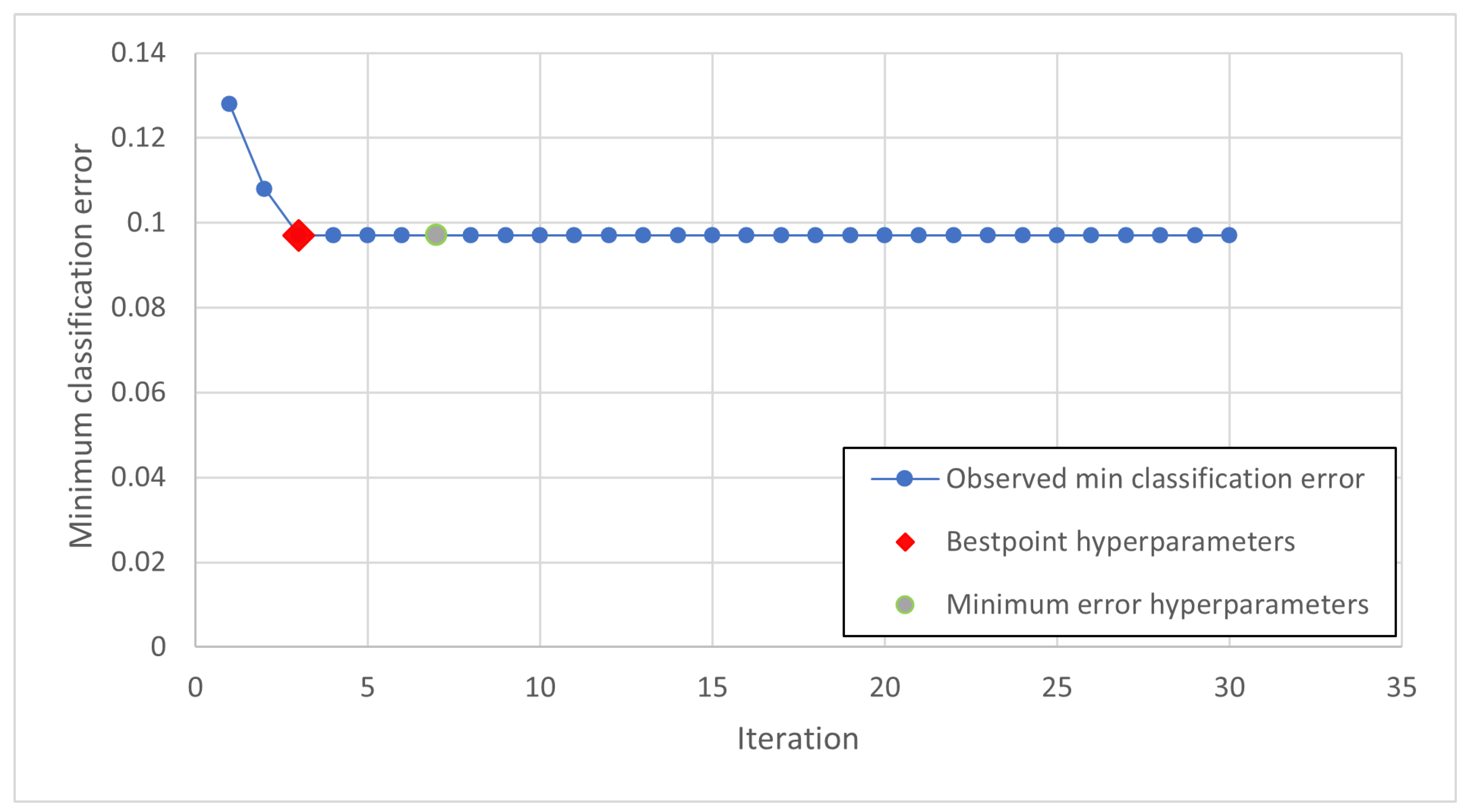
The training phase is therefore carried out iteratively and it is necessary to introduce criteria with which to terminate it. The iterations can be limited in number, in time or on the basis of an index and the achievement of its threshold value.

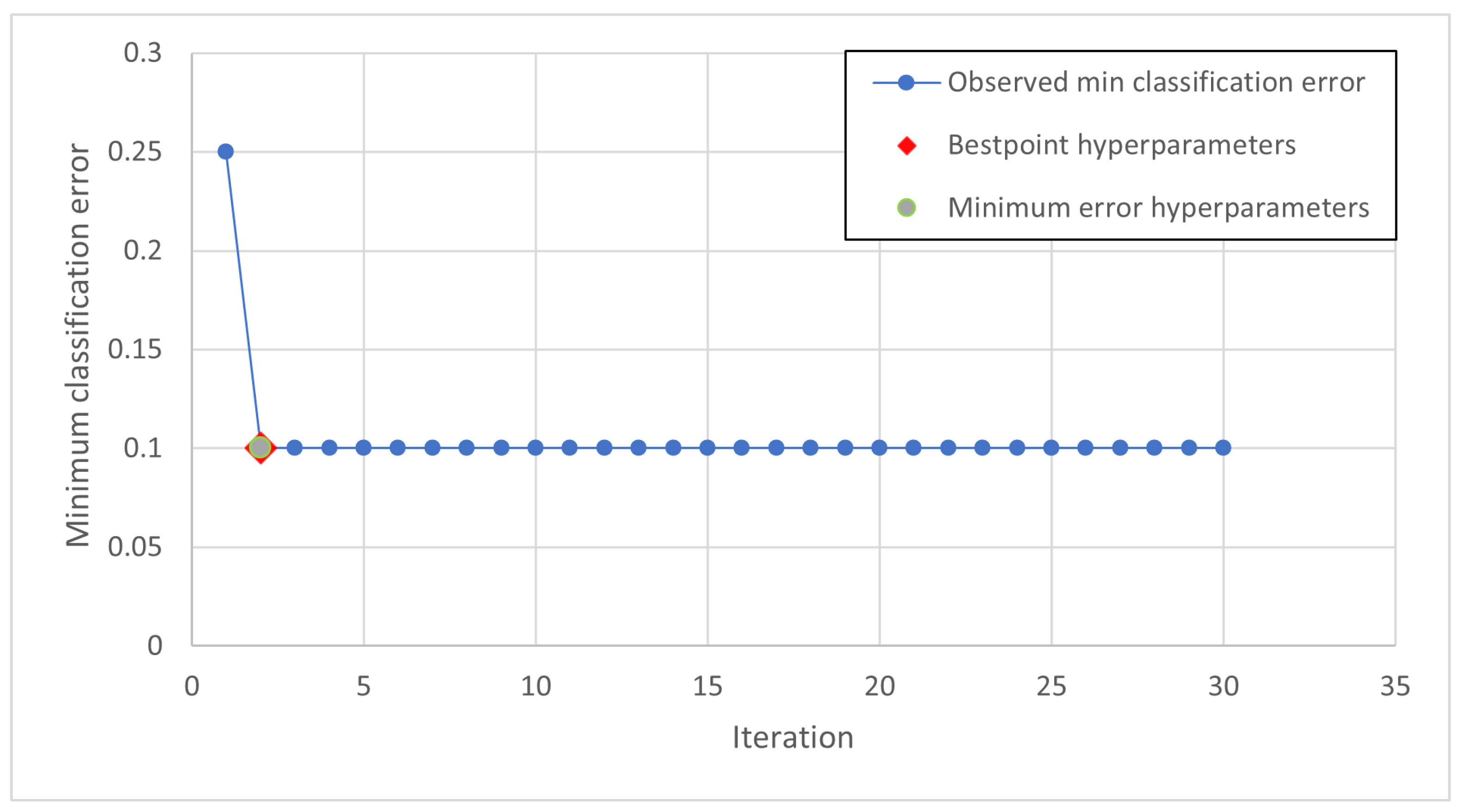
The graph in the plot represents the estimate of the minimum classification error (MCE). The MCE is calculated considering the sets of hyperparameter values for each iteration (blue points). The yellow dot and the red square represent the minimum error hyperparameters and the bestpoint hyperparameters, respectively. In Figure 9, the minimum error Hyperparameters and the bestpoint hyperparameters coincide.

The optimized hyperparamete configuration obtained in the case study is reported in

Table 5. Optimized hyperparameter configuration.

Hyperparameter	Range
Number of Fully Connected Layers	1
First Layer Size	10
Activation	$ReLU$
Regularization Strength (Lambda)	0
Standardize Data	Yes

.

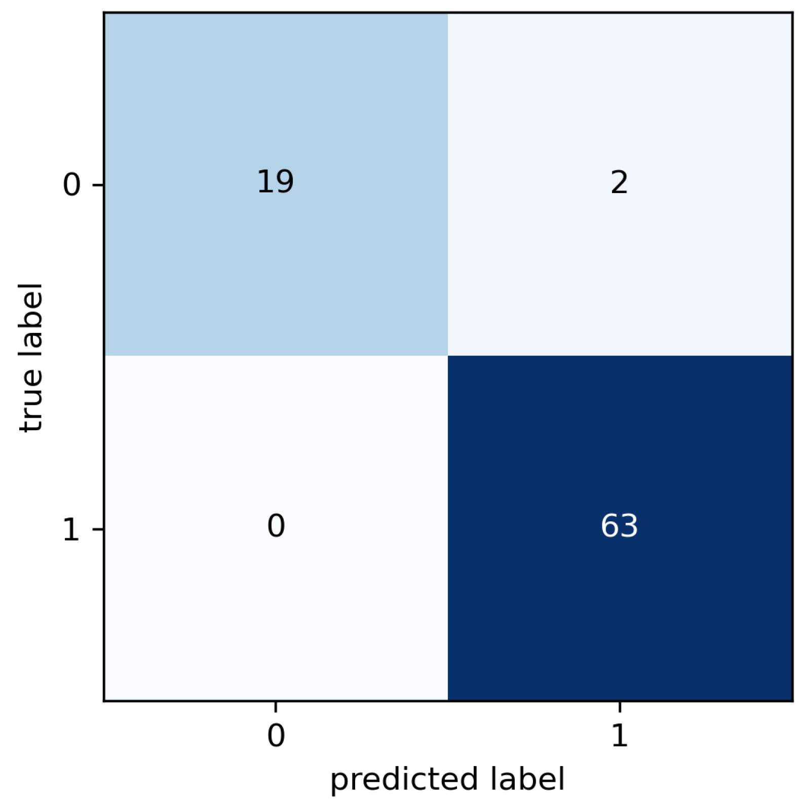
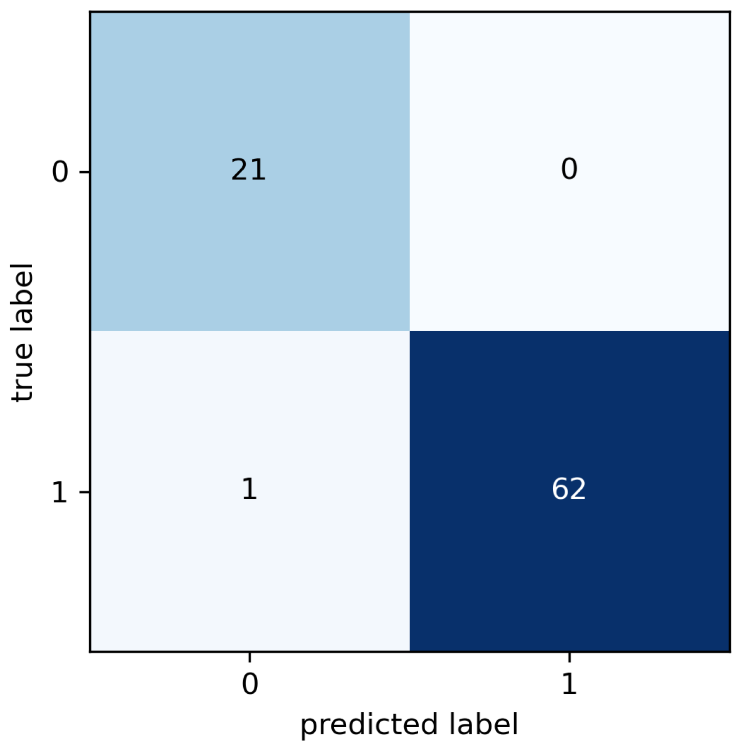
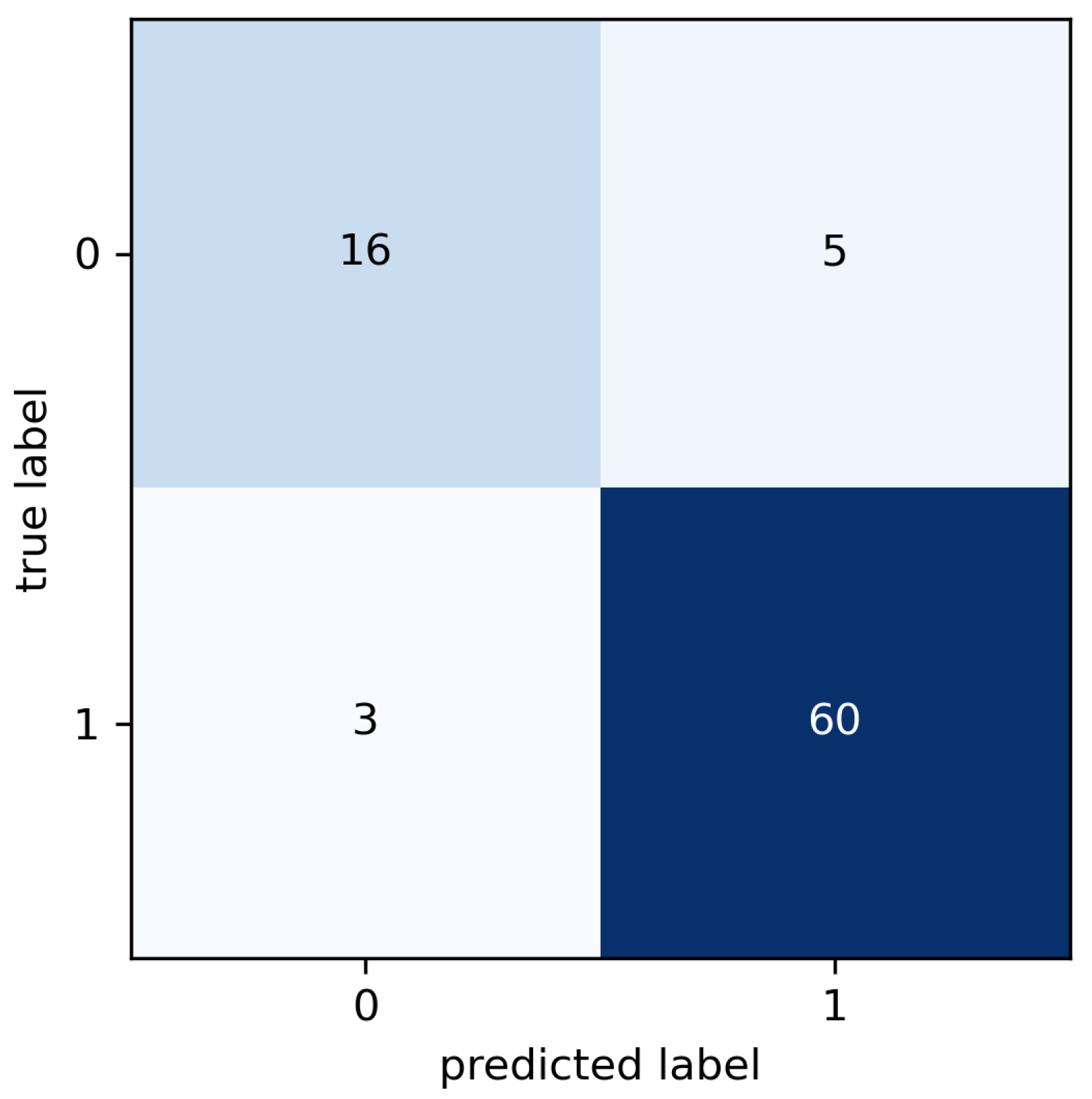
The results of the cross validation are summarized in the confusion matrix (Figure 10) where known and predicted classes are reported. The false classes (labeled as 0) correspond to observations labeled as healthy, that is, observations collected from the motors in good condition. The true classes are the classes labeled as faulty, i.e., observations corresponding to motors in anomalous conditions (broken bearings, misalignments, etc.).

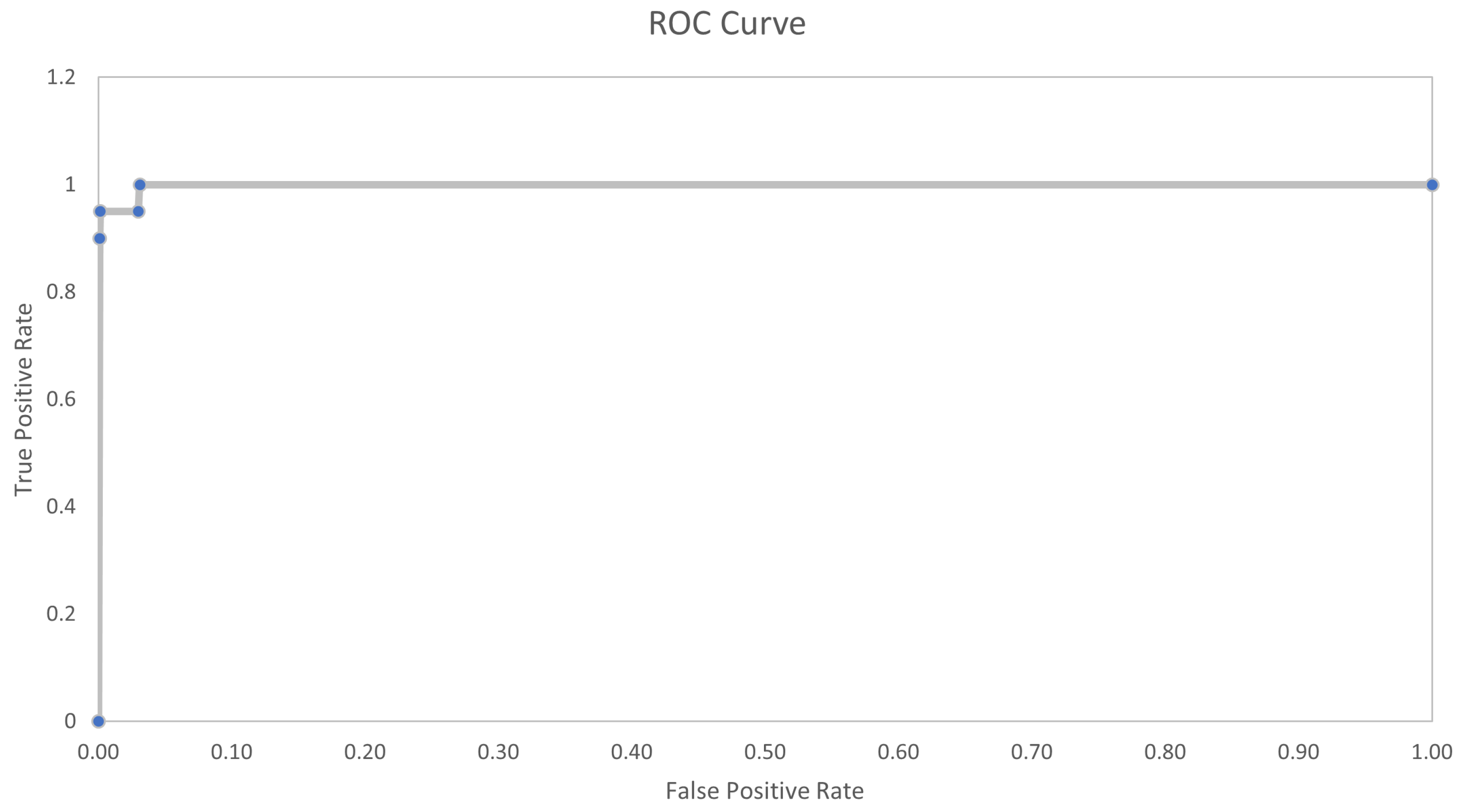
Figure 11 shows the receiver operating characteristic (ROC) curve which represents the relationship between sensitivity (true positive rate) and specificity (true negative rate).

The sensitivity is calculated by taking the ratio between the cases belonging to the class of fault signals correctly classified as positive (the true positives) divided by the sum of true positives and the faulty cases erroneously classified as negative (the false negatives) (5) [25]. This index represents the probability with which a classifier correctly identifies a faulty case as positive.

$$\mathrm{Sensitivity}=\frac{\mathrm{True}\mathrm{Positives}}{\mathrm{True}\mathrm{Positives}+\mathrm{False}\mathrm{Negatives}}.$$

(5)

The specificity is calculated by taking the ratio between the cases belonging to the class of nominal device signals correctly classified as negative (the true negatives) divided by the sum of true negatives and the healthy cases erroneously classified as positive (the false positives). This index represents the likelihood with which a classifier correctly identifies a healthy case as negative.

$$\mathrm{Specificity}=\frac{\mathrm{True}\mathrm{Negatives}}{\mathrm{True}\mathrm{Negatives}+\mathrm{False}\mathrm{Positives}}.$$

(6)

Both sensitivity and specificity indices are calculated from the results presented in the confusion matrix in Figure 10.

5.3. Performance Comparison

A comparative analysis was carried out between the results provided by the proposed method and those obtained by replacing the machine learning core with two common classifiers. The selected algorithms for this comparison were chosen for their characteristic of being widely used in diagnostic applications based on the machine learning approach. In particular, the solution based on a feed-forward neural network has been compared with the support vector machine (SVM) and decision tree (DT).

The support vector machine is a binary classifier trained on a set of labeled patterns [26]. A training set can be defined as:

$$({\mathit{x}}_{\mathit{i}},y_i)\in R^l\times \{\pm 1\}i=1,\dots ,N$$

(7)

where ${\mathit{x}}_{\mathit{i}}\in R^l$ is the input dataset and $y_i\in \{\pm 1\}$ is the target. The goal of the support vector machine is to divide the samples by a hyperplane so that the division coincides with the targets $y_i$.

The classification function is defined as:

$$f\left(\mathit{x}\right)=sgn(\mathit{w}·\mathit{x}+b).$$

(8)

The function $sgn$ is the bipolar sign function, the vector w is the vector of coefficient and b stands for the bias of the hyperplane.

The classifier hyperplane must be identified in order to satisfy the condition that $y_i$ is greater than or equal to one:

$$y_i[\mathit{w}·\mathit{x}+b]\ge 1,i=1,\dots ,N.$$

(9)

Equation (9) can be modified as reported in Equation (10), in order to introduce a slack variable to identify a hyperplane that does not fully satisfy Equation (9) but maximizes the result.

$$y_i[\mathit{w}·\mathit{x}+b]\ge 1-e_i,i=1,\dots ,N.$$

(10)

The goal of the algorithm is to minimize the following:

$$min\mathit{J}(\mathit{w},e,b)=\frac{1}{2}\mathit{w}·\mathit{w}+\frac{1}{2}C\sum _{i=1}^N{e}_i^2.$$

(11)

As performed in the case of the neural networks described above, in this case, for comparative purposes, we proceeded with the evaluation of the performances with the cross validation technique. The random search technique was also applied to the support vector machine for the configuration of the hyperparameters. The possible values that the hyperparameters can assume are shown in

Table 6. Hyperparameter configuration—SVM.

Hyperparameter	Range
Box Constraint Level	{0.001–1000}
Kernel Scale	{0.001–1000}
Kernel Function	{Gaussian, Linear, Quadratic, Cubic}
Standardize Data	{True, False}

.

Following the application of the random search, the optimal configuration obtained consists of a kernel function such as the Gaussian, a kernel scale of 12.6062, a box constraint level of 167.007 and standardize data as true (Figure 12). This optimal configuration allowed for reaching an accuracy of 97.6%, true positive rate of 100% and true negative rate of 90.4% (Figure 13).

The support vector machine ROC curve is shown in Figure 14. The curve is quite similar to that obtained with the feed-forward neural network proposed in the method, in fact, the accuracy level achieved is not much lower. This does not mean that the feed-forward neural network is the best choice for predictive maintenance purposes in asynchronous three-phase electric motors.

Decision trees are machine learning algorithms that can be used for both regression and classification problems. A decision tree is a tree-like model of decisions and it is usually built upside down with its leaves at the bottom.

In decision trees, decisions are represented by the path taken from the root to the leaf node. Tree construction occurs iteratively through leaf splitting or pruning. The random search and cross validation techniques have also been applied in the case of decision trees [27]. The possible values that the hyperparameters can assume are shown in

Table 7. Hyperparameter configuration—decision tree.

Hyperparameter	Range
Maximum Number of Splits	{1–83}
Split Criterion	{Gini   Diversity  Index; Maximum Deviance  Reduction}

. It is necessary to establish the optimal split criterion for this case. This choice will also be made by means of the random search technique. Two split criteria are considered: Gini diversity index and maximum deviance reduction function. The Gini index (G) is defined according to Formula (12):

$$G=1-\sum _k{P}_k^2,$$

(12)

where the percentage inside a group of elements is defined as $P_k$ and the group of elements must belong to class k [28]. The value G represents the purity and it is equal to 0 if all the elements (inside the group) are part of the same class. Thus, from the branches the node returns an output observation of just one class and, if all the elements belong to that specific class, the classification error is null.

The other split criterion is the maximum deviance reduction ($MDR$) function (sometimes called cross entropy). The function is defined as:

$$MDR=-\sum _k{p}_k\ast lo{g}_2\left(p_k\right).$$

(13)

In the maximum deviance reduction function, the elements that are part of the class k are represented by the variable $p_k$ which stands for the percentage inside a group [29]. The procedure of splitting keeps going if the conditions are still valid. Of course, a too complex decision tree is not advisable and must be avoided, otherwise there could be risks of overfitting, poor interpretability and unreliability of predictions.

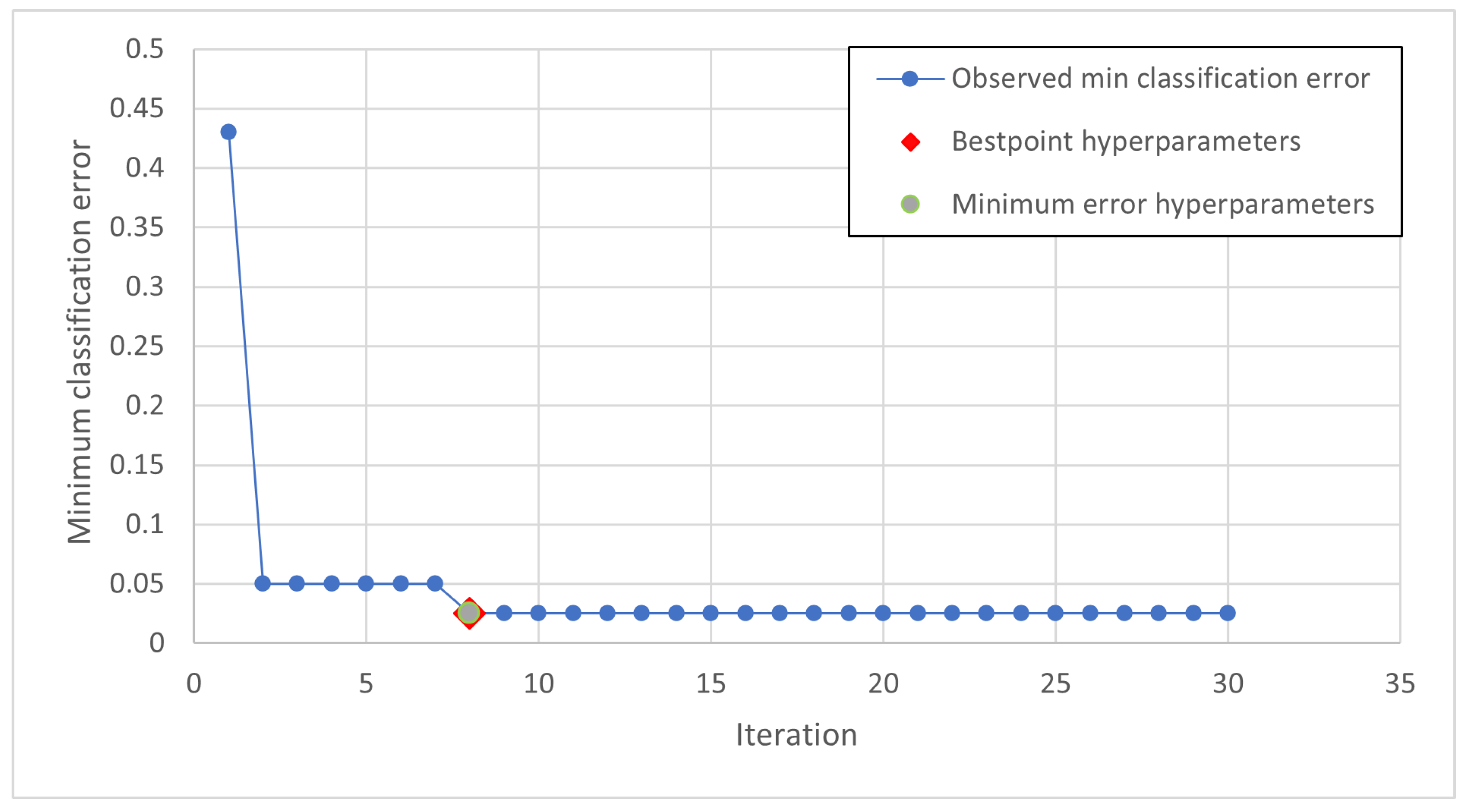
Following the application of the random search in the decision tree algorithm, the optimal configuration obtained consists of six splits and the Gini diversity index as the split criterion (Figure 15). This optimal configuration allowed for reaching an accuracy of 90.5%, true positive rate (sensitivity) of 95.2% and true negative rate (specificity) of 76.2% (Figure 16).

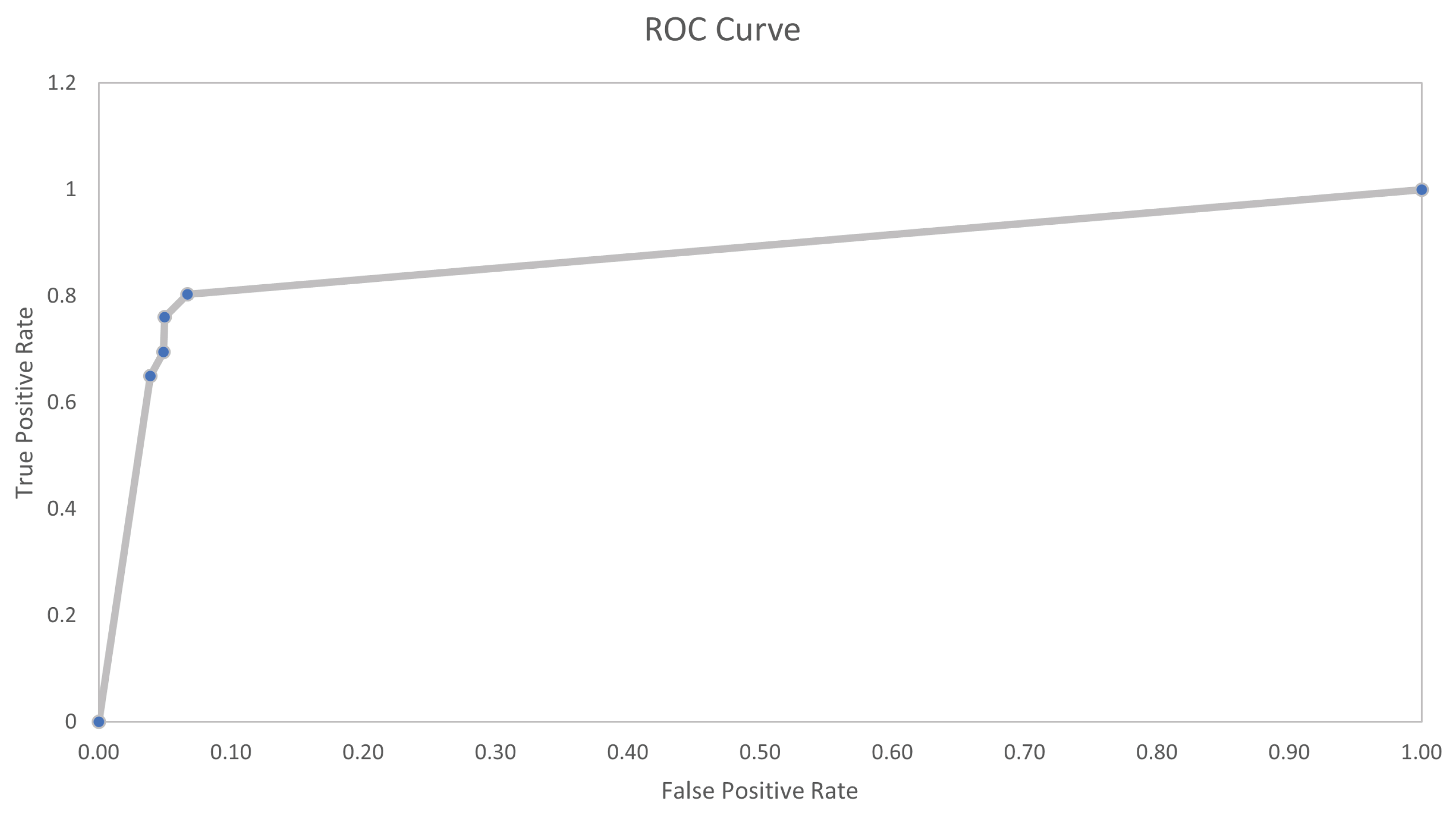
Figure 17 shows the ROC curves of the decision tree model. It is possible to note that the area under the curve is considerably smaller than that of the curves in the two previous models. This suggests that the performances cannot be superior or equal to those of the other two algorithms previously explored. Perfomance comparison is summarized in

Table 8. Performance comparison.

Model	Accuracy	Sensitivity	Specificity
Feed-Forward Neural Network	98.8%	98.4%	100%
SVM	97.6%	100%	90.5%
Decision Tree	90.4%	95.2%	76.2%

.

5.4. Further Comparisons with State-of-the-Art Solutions

Additional comparisons, in terms of performance, were carried out by comparing the results published in the literature. An exhaustive comparison is not easy to make as the methods proposed as the state of the art generally have more than one characteristic different from those that make up the method proposed in this work. In order to carry out a suboptimal comparison, all selected works are based on samples coming from the supply current signals.

The authors of [30] have proposed a multi-stage approach based on an MLP-ANN machine learning algorithm capable of detecting fault causes in induction motors.

The authors of [31] have proposed a method based on a frequency plot-based convolutional neural network (FOP-CNN) for detecting motor faults. The study was performed under different workloads.

The authors of [32] have proposed a method based on an unsupervised technique whose advantage is learning from the dataset without an external intervention for data labeling. The machine learning algorithm is based on a CNN. The work is focused on bearing faults and no information was provided regarding other kinds of faults.

The authors of [33] have proposed an empirical wavelet transform convolutional neural network (EWT-CNN). The method proposed in the work achieves 97.3% accuracy.

All the methods reported in this comparative subsection have been validated on case studies limited to a few units of faulty motors. Moreover, papers considered in

Table 9. Comparison with literature methods based on ML and current samples.

Method	ML Classifier	Accuracy	Case Study Motors
Bazan et al. [30]	MLP-ANN	96%	2 Motors
Piedad et al. [31]	FOP-CNN	92.4%	5 Motors
Lei et al. [32]	CNN	99.6%	1 Motor
Shao et al. [33]	EWT-CNN	97.3%	6 Motors
Proposed Method	ANN	98.8%	28 Motors

do not provide a complete description of the adopted sensors and sample acquisition technologies. Therefore, it is not possible to hypothesize the absence of overfitting of the trained models.

6. Conclusions

In this paper, a method for the predictive maintenance of three-phase asynchronous electric motors has been proposed. The proposed method explores the acquisition techniques for samples of current measures on the supply power lines. The proposed method is based on an analysis carried out on each single phase. For each motor, the three phases are used independently in this method. This approach increases the robustness of the method as a problem that can occur in a single phase can be identified by the algorithm. Furthermore, treating the phases separately allows for tripling of the size of the dataset, reducing the risk of overfitting.

The preprocessing for feature extraction is also easily implemented in edge computing devices, which allows the implementation and deployment of the proposed method even in real-world contexts where access to external resources is limited. The machine learning algorithm adopted in this method is a classifier based on a feed-forward neural network. The simplicity of this model is advantageous for edge computing deployment.

Finally, in this work a further comparison was made between the performance of the feed-forward network-based classifier and other common classifiers in order to demonstrate the better performance that a feed-forward-based classifier is capable of achieving. It is evident from the experimental data that the proposed method achieves high levels of accuracy (higher than $98\%$) and a sensitivity typically greater than $98\%$.

As for the method limitations, its main weakness is the large dataset required for its training; it would be hard to find such a large number of faulty motors. Furthermore, it is not yet possible to provide information on the nature of the fault affecting the engine to drive maintenance more specifically. This problem is currently under study by focusing on reinforcement learning techniques [34]; results will be presented in the future.