Article

Retrofitting Buildings into Thermal Batteries for Demand-Side Flexibility and Thermal Safety during Power Outages in Winter

Department of Architecture and Urban Studies, Politecnico di Milano, 20133 Milano, Italy
*
Author to whom correspondence should be addressed.
Energies 2022, 15(12), 4405; https://doi.org/10.3390/en15124405
Submission received: 16 April 2022 / Revised: 7 June 2022 / Accepted: 9 June 2022 / Published: 16 June 2022
(This article belongs to the Special Issue Sustainable Renovation and Energy Retrofit in Buildings)

Abstract

:
Decarbonizing heating in buildings is a key part of climate change mitigation policies, but deep retrofit is progressing slowly, e.g., at a pace of 0.2%/y of the building stock in Europe. By means of tests in two flats of a multiapartment housing complex recently renovated to very low values of energy needs, this paper explores the role of deep retrofitted buildings in providing energy flexibility services for the occupants/owners/managers and for the energy system. Key to this flexibility increase and capacity savings is the large reduction of energy needs for heating via a high level of external insulation, which allows the thermal capacity of the building mass to act as an energy storage, without the large energy losses presently affecting a large part of the building stock. Due to the limited number of case studies reporting experimental applications in real buildings, this research aims to offer an analysis based on a series of tests and detailed monitoring which show a significant increase in the time interval during which the low-energy-needs building remains in the comfort range, compared to a high-energy-needs building, when active delivery of energy is deactivated during the heating season. Intermittent renewable energy might hence be stored when available, thus enhancing the ability of the energy system to manage inherent variability of some renewable energy sources and/or increasing the share of the self-consumption of locally generated RES energy. Besides, two unplanned heating power outages which have involved the entire building complex allowed us to verify that deep retrofitted buildings are able to maintain thermally safe indoor conditions under extreme events, such as a power outage, for at least 5 days.

Graphical Abstract

1. Introduction

1.1. Research Background

Reducing the peak loads and shifting the demand to mitigate the effects of power outages have been gaining increasing attention, which has resulted in the developing of methods and technologies for energy storage in the system [1]. At the same time, the integration of renewable energy sources (RES) is one of the main challenges for the future global energy supply, and in this regard energy storages can effectively contribute, allowing excess energy produced from RES at certain times to be stored and used at later moments of lower RES availability or higher demand.
Among the different types of energy storage, thermal energy storage (TES) is a technology being increasingly studied for buildings and communities [2,3,4]. A thermal storage allows stocking thermal energy by heating or cooling a medium so that the stored energy can be used at a later time for heating and cooling applications or power generation. TES techniques in buildings can be categorized as passive or active: in passive storages, such as the thermal capacity of the building fabric itself or the heat of phase transition using phase change materials (PCM), the driving force for charging and discharging the storage medium is only the temperature difference between the storage and the surroundings. In the case of an active storage, such as storage tanks in the HVAC system or active storage in the building structure as TABS (thermally activated building systems) [3], the charging and discharging occurs with active help from pumps or fans.
Several studies have been developed in the last few years to investigate the potential of TES in the building sector in relation to the emerging topic of building energy flexibility [5]. Some authors have focused their studies on analyzing the flexibility provided by the structural thermal mass of the buildings [6,7,8], sometimes indicated with the concept of Building as Battery (BaB) [9], while others have investigated the load flexibility capacity of PCM integrated into the building envelope [10] or in furniture [11]. Growing interest has also been found in assessing the energy flexibility potential provided by active thermal storages [12,13]. Other studies have investigated combined passive thermal mass and active storage to investigate the demand response potential of buildings [14]. In parallel, metrics and quantification methodologies for energy flexibility applied to TES have been developed [15,16].
As shown from the literature review, the role of TES in buildings in supporting the penetration of renewable energy sources is clearly recognized; however, there is a need for increasing knowledge and demonstrating how much energy flexibility different buildings may be able to provide to the future energy networks, especially in extreme conditions, such as prolonged power outages.
The International Energy Agency (IEA)—Energy in Buildings and Communities Programme (EBC) research project ‘‘Annex 80: Resilient Cooling of Buildings” [17] identifies power outages as one of the major disruptions that can influence occupant indoor thermal quality conditions on the building scale, and stresses the importance of developing indicators of thermal resilience in order to assess passive and active solutions to provide comfort in buildings.
This paper investigates the energy flexibility potential offered by the structural thermal capacity in energy-retrofitted buildings and aims at showing the less visible benefits that an energy renovation can bring to the energy network.
In fact, not all the buildings are capable of providing the same amount of energy flexibility due to the characteristics of the envelope which affect the storage capacity and the duration of the period of modulation. The maximum thermal energy storage potential of a building is mainly determined by its total effective thermal capacity. However, Johra et al. [11] conclude that the envelope insulation level is the most important building parameter with respect to the capacity of a dwelling to shift its heating use in time. In particular, as shown by Le Dréau et al. [8], poorly insulated buildings are capable of modulating large amounts of heat but just for short periods of time, and they suffer high losses, thus corresponding to low storage efficiency. On the contrary, well-insulated buildings can modulate smaller amounts of heat but are capable of managing longer periods of modulation with high efficiency. Similarly, Foteinaki et al. [6] showed that low-energy buildings are highly robust and can remain autonomous for several hours.
In Europe, a large portion of the building stock is characterized by poorly insulated buildings which cannot take part in the flexibility logics before undergoing a deep energy retrofit. Specifically, 85% of the European building stock, which corresponds to more than 220 million building units, was built before 2001 and more than 40% before 1960. Almost 75% of it is energy inefficient according to current building standards, and 85–95% of the buildings that exist today will still be standing in 2050. The renovation rate is still low and has low effects on final energy use, while it represents one of the main pillars of the EU commitment to reduce climate-altering emissions by 55% by 2030 and to reach climate neutrality by 2050 [18].
The Renovation Wave published in 2020 develops a systematic action plan with the aim to at least double the annual energy renovation rate of residential and nonresidential buildings by 2030, which will result in 35 million building units, and to foster deep energy renovations. Among the priorities, the renovation strategy focuses on public buildings and social infrastructures which should serve as a role model and reference point for the industrialization of construction and the cobenefits that could become immediately visible to the public. In fact, the Open Public Consultation on the Renovation Wave [19], published in 2020, points out that in residential buildings, insufficient understanding of energy use and savings is rated as a very important/important barrier by more respondents than any other barrier, highlighting the need to effectively communicate the benefits of energy retrofits to encourage the energy renovation of the building stock [20].
In the literature, a certain number of data and analyses on the energy performance effects of deep retrofits are available [21], even though there are uncertainties about the reported savings due to a lack of uniform nomenclature and definitions. More recent is the investigation of the potential of energy-retrofitted buildings in contributing to deliver energy flexibility at the level of the buildings or the district [22]. This flexibility can then be exploited for demand-side flexibility actions and allow for several benefits: enhanced possibilities of self-use of locally generated renewable energy, reduction of demand in coincidence with system peaks, adaptation to climate change, and more frequent and violent extreme weather events.
The latter case falls under the definition of “thermal safety” or “passive survivability”, which refers to the building’s ability to maintain livable conditions when energy sources are cut off [23]. The frequency and intensity of extreme events has increased over the last decades, and in Europe, the global warming scenarios will likely undergo a further intensification [24]. Various voluntary certification schemes, such as LEED, are testing resilience indicators such as “passive survivability (thermal safety)” [25]. The RELI resilience rating system [26] allocates credit points to “thermal safety during emergencies”, requiring indoor temperatures to be at or below outdoor temperatures in the summer, and above 10 °C in the winter for up to four days, in absence of active energy supply. In this paper we adopt the term “thermal safety”, except when we quote literature that uses other terminology to name this concept.
Given this background, the paper emphasizes the benefits of energy flexibility given by retrofitted buildings for the overall energy system which might add impulse to the European “Renovation wave” and foster climate protection, when properly integrated in legislation and the regulation of markets.
In this paper, we focus on flexibility and thermal safety in the winter season since heating is still a high portion of final energy use in Europe, and many regions are heating dominated. In particular, the investigated case study is located in Milan which, according to the updated table in D.P.R. 412/1993 [27] on climatic zones, is classified in zone E with heating degree days (HDD) during the heating season (for Milan it is from 15 October to 15 April) ranging between 2101 and 3000 K·d, considering a base temperature equal to 20 °C. For cooling degree days (CDD), there is no explicit method chosen in the Italian legislation. However, references in literature [28] find values of about 100–150 K·d, assuming a base temperature of between 24 °C and 26 °C. Having set up the measurement and data logging systems, we will also be running flexibility tests in the same building during summer.
Section 1.2 presents a review about the most relevant TES applications using building thermal mass available in literature. Section 1.3 highlights the research contribution.

1.2. Literature Review on TES Using Building Thermal Mass

The activation of the structural thermal mass of a building as thermal energy storage is not new in literature [29,30]. However, more recently, the potential of structural thermal mass has been explored as a way to provide energy flexibility [6,8,31], i.e., allowing the building to be independent from the energy network for a certain number of hours while guaranteeing adequate indoor comfort conditions. The literature analysis shows that the majority of studies use dynamic simulation to discuss the potential exploitation of TES features [6,8,32]. Fewer studies present results of field measurements [9,33,34,35]. Additionally, the majority of the studies focused on modulation events during the heating season, e.g., in [6,7,32], while fewer papers have deepened this strategy during the summer, e.g., in [31,36]. Johra et al. [7] developed research on the effect of indoor items and furniture, showing that their effect is limited for medium- and heavy-structure cases but not negligible for light-structure buildings. A growing interest is found on the analysis of controls for energy flexibility using thermal mass [37,38]. Moreover, some authors have proposed and applied metrics and methodologies to quantify the impact of this strategy [16,39].
Even if the use of the thermal mass as energy storage cannot reduce the seasonal mismatch between demand and, e.g., solar RES generation [30], it allows load-shifting up to several days. However, the majority of the studies focus on “short term” events limited to a few hours (from 2–3 h up to maximum 24 h, some including both the charging phase of the thermal mass and the discharge, others only the discharge), while examples showing “long term” performances (with load-shifting lasting more than one day) are few and rely mainly on simulated data.
For example, Erba and Pagliano [22] show the variation over time of the operative temperature in a heated flat as a function of the retrofit measures undertaken, after two days during which the heating system was kept on (before being turned off) and with the cyclic repetition of an “average winter day”. In that analysis, flexibility offered by “long term” passive thermal storage is one of the necessary elements, combined with efficiency and sufficiency, for achieving a zero-energy balance (defined in physical terms, not only as an accounting exercise) of a district with little or zero land take outside the footprint of the district.
Annex 80 also analyzes the resilience at various time scales, including events of duration of several days, and proposes definitions and terminology. Attia et al. [17] explored various time and space scales, focusing in particular on the building scale. Zhang et al. [40] presented a review of available passive technologies from the point of view of resilience capacities, applicability, and technology readiness. Among these techniques, thermal mass is also briefly analyzed, pointing out the fact that thermal losses of the storage might constitute a limitation for the application. In the present paper, we focus on the role of thermal mass available in the building fabric and the role of insulation.
Homaei and Hamdy [41] explored, through energy simulations, the winter passive survivability of a representative Norwegian single-family house during the coldest week using a typical weather file (IWEC) suggesting ten different building designs by changing the design parameters. Wilson [42] discussed, in his study on thermal habitability of buildings during power outages, the analysis published by the Urban Green Council [43] on six different residential building types during week-long power outages under typical summer and winter conditions. These buildings were modelled assuming typical building stock and energy code compliance. Ozkan et al. [44] simulated the passive survivability performance for eight days after a power failure of an apartment unit in Toronto during typical summer and winter weeks selected from typical meteorological-year data in the EnergyPlus Weather file.
Table 1 presents an overview of the most significant cases available in the literature, with a focus on the duration of the modulation event as a measure of performance. A similar approach is adopted in this manuscript.
The table reports the scope of the study, the method (i.e., simulations or/and on-site measurements), the type of building, the strategy of thermal storage (type of service and period of charging of the thermal mass), and the main results. These last are expressed, where possible, showing the duration of the load-shifting after the power outage. In the remaining cases, the results are expressed in terms of available key performance indicators. Additionally, it is indicated if the study develops the analysis by referring to building energy flexibility.

1.3. Research Contribution
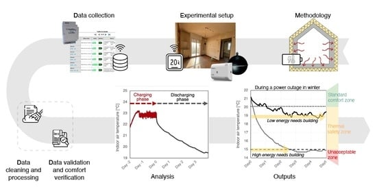
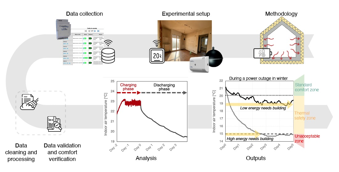
This paper aims to analyze the behavior of retrofitted buildings during the heating season when their thermal capacity is used as thermal energy storage by postponing the energy use for heating for a certain period of time while maintaining adequate thermal comfort conditions in the building.
The literature analysis pointed out that the majority of studies focused on TES applications which show load-shifting generally of a few hours up to maximum one day. While recognizing the usefulness of those, especially under the assumption of relying solely on renewable sources, such as PV systems, this paper investigates the potential for longer shifts, in which the building still remains within the comfort range, and for the possibility to protect occupants of buildings during events which may disrupt the supply of electricity and/or fuel for a number of days, or to integrate RES when they show variability over a certain number of days up to a week.
The paper uses a time-based metric as a measure of performance, as emphasized in [44], to provide information on the thermal comfort autonomy which can be offered by retrofitted buildings considering standard indoor comfort thresholds, as indicated by the standard EN 16798–1:2019 [54], and the thermal safety under extreme conditions, such as a power outage, where an acceptable range is considered simply on what is safe for occupation.
Due to the limited number of case studies reporting experimental applications in real buildings, the research aims at offering an analysis based on measured data to show the long-term performance in real cases. Further, the studies available in the literature presenting the results of experimental research are generally based solely on the measurement of indoor air temperatures [9,33,34,35]. This paper, to verify the assumption of considering the air temperature as sufficiently representative of the operative temperature of the indoor environment in buildings characterized by a well-insulated envelope, presents a comparison between: (I) the operative temperature calculated considering the mean radiant temperature obtained through the use of the globe thermometer; (II) the operative temperature, calculated using the mean radiant temperature calculated from measured values of the temperature of the internal surfaces of the surrounding walls, their area, and their view factor between the chosen position in the room and the surfaces; and (III) the measured air temperature. Additionally, the analysis includes the measurement of the temperatures in the surroundings spaces (e.g., the stairs and adjacent apartments), which is not commonly found in literature.
The study also offers, for the first time to the authors’ knowledge, an assessment of the potential of the thermal mass based on measured data after an energy interruption in a whole apartment block comprising a large number of flats. This allows one to evaluate the difference in the behavior of the single apartments, while most of the studies are limited to a single thermal zone.
Finally, the paper, investigating a public, multifamily residential building that had recently undergone a deep energy retrofit, serves as a demonstrative example in response to the priorities highlighted by the strategy put in place to stimulate the Renovation Wave [18].
The paper is structured as follows: Section 2 describes the research methodology, which includes an experimental phase and a demonstration phase. In Section 3, the apartment block case study, the experimental setup and the demonstrative environment are presented. In Section 4, the results are shown. Section 5 discusses the investigated benefits of deep retrofit for the energy system and outlines plans for the future work. Finally, Section 6 presents the conclusions.

2. Methodology

In this section, the methodology followed in the research to assess the “long-term” potential of the building thermal mass in a multiapartment retrofitted building is outlined. Figure 1 shows the conceptual study framework from the definition of the method to the outputs. On the basis of the literature review, the configuration of the monitoring system was defined and implemented, and the steps of data collection, cleaning, processing, validation, and analysis are outlined.
The paper presents an experimental phase, carried out at the level of single flats under controlled conditions, and a demonstration phase which occurred in the entire building complex during standard operating conditions.
In both cases, the evolution of the indoor air temperature during the charging and discharging of the storage medium, i.e., the building thermal mass, was analyzed to be able to calculate the number of hours the building can remain in a specified comfort range without active energy input. In the experiments, an increased set-point within the limits of indoor thermal comfort was defined to allow the introduced additional heat to be stored in the building fabric. In the demonstration phase, the complex, while running under standard operating conditions, has undergone an energy interruption of several days, which has allowed for the verification of the thermal behavior of all the buildings after a complete shut off of the heating system. In both cases, the analyses show the results considering standard comfort thresholds as well as thermal safety thresholds.

2.1. Experimental Phase: Flat Level

The experiments were carried out in 2 of the 66 apartments of the building complex described in Section 3.1, under different outdoor weather conditions and charging conditions, to analyze the effects of different forcing factors on the building. Besides, the two flats are characterized by different orientations and floor areas, in order to capture some of the variability of the building’s thermal behavior. The flats were kept unoccupied and without furniture. This made it possible to, on one hand, avoid any disturbances to the measurement by the occupants, and on the other it prevented the full exploitation of the thermal masses available, such as the elements with thermal capacity inside the accommodation (e.g., furnishings). Further, the tests were conducted while keeping the mechanical ventilation in extraction mode only. This choice was made according to the assumption that during extreme events, the building must be able to guarantee thermally safe conditions when the energy sources are limited. Additionally, the tests attempted to accurately reproduce the existing conditions of the building, which is currently operating in extraction mode only, in order to be comparable with the actual situation during the demonstration phase. In the future work, as detailed in the discussions, different conditions, including occupants’ presence and the full activation of the mechanical ventilation, including heat revery on exhaust air, will be tested.
The experimental set up was designed according to international standards which refer to the operative temperature for the evaluation of thermal comfort (experimental setup phase as in Figure 1). Operative temperature is defined as the uniform temperature of an enclosure in which an occupant (in a certain position) would exchange the same amount of heat by radiation plus convection as in the existing, nonuniform environment. According to EN ISO 7726 [55], where the relative velocity is small (<0.2 m/s) or where the difference between mean radiant temperature (MRT) and air temperature is small (<4 °C), the operative temperature can be calculated with sufficient approximation as the mean value of air and mean radiant temperature. MRT is defined as the uniform temperature of an imaginary enclosure in which radiant heat transfer between the surfaces of the enclosure and a person (in a certain position) is equal to the radiant heat transfer in the actual nonuniform enclosure. It can be assessed by measuring globe temperature, air temperature, and air velocity, according to ISO 7726 [55]. Measurement of air velocity under conditions of free convection is not necessary, due to its reduced value and its variability. ISO 7726 offers the following Formula (1) for this case:
MRT g = [ ( t g   + 273 ) 4 + 0.4 · 10 8 | t g t a | 1 4 · ( t g t a ) ] 1 4 273
MRT can also be calculated from measured values of the temperature of the surrounding walls, their area, and their position in relation to a person (calculation of geometrical shape factors, Fp-j, where p identifies the person and its position within the room, and j 1 to N identifies the various surrounding surfaces), according to Formula (2):
MRT s = [ T 1 4 F p 1 + T 2 4 F p 2 +   T N 4 F p N ] 1 4
Thus, in the experiments, the following quantities were measured with a time-step of 10 min: air temperature and globe-thermometric temperature in the center of the room and surface temperature of each wall and window (data collection phase as in Figure 1). The detailed description of the sensors is presented in Section 3.2. In parallel, the outdoor air temperature and global solar irradiance were registered during the experiments.
The thermal comfort range was defined considering standard comfort thresholds as well as thermal safety thresholds in winter. In the first case, in order to determine the comfort range, in terms of operative temperature, reference was made to the Standard EN 16798-1:2019 [54] selecting category II and assuming typical indoor winter conditions. Using the online thermal comfort tool of the University of California, Berkeley [56], which incorporates the algorithm of the Fanger model, comfort category II ranges in winter between 20.1 °C and 24.5 °C in terms of operative temperature. To define the lower thermal safety threshold after a power failure, reference was made to the ASHRAE transactions—2016 [57] that defines the passive survivability in winter as the time between when heating is shut off and when the indoor operative temperature reaches 15 °C from an original heating setpoint of 21 °C.
The experiment starts with a phase of charging which considers an increased set-point for a certain time duration, during which all or part of the introduced, additional heat can be stored in the thermal mass of the building. After switching off the heating system, the building remains independent from active energy supply, either for networks or local RES generation, for a certain period. During the charging and discharging phase the indoor air temperature, globe-thermometric temperature, and surface temperature are recorded.
A comparison between operative temperatures and air temperature was performed to verify if in buildings characterized by a well-insulated envelope the air temperature can be sufficiently representative of the operative temperature of the indoor environment (data validation phase as in Figure 1). In particular, the following three quantities were compared: the operative temperature Top,g, calculated considering the mean radiant temperature obtained through the use of the globe thermometer; the operative temperature Top,s, calculated using the mean radiant temperature calculated from measured values of the temperature of the internal surfaces of the surrounding walls, their area, and their view factor between the chosen position in the room and the surfaces; and the measured air temperature Ta. The absolute and relative difference between operative temperature and air temperature was calculated as | Δ T | = | T o p T a | and Δ T = T o p T a . The absolute difference describes the magnitude of the difference between operative temperature and air temperature, regardless of which is cooler or warmer. The relative difference provides the actual observed differences in temperature during the test, with signs.
Moreover, in the experiments, the temperature drifts were assessed (comfort verification phase as in Figure 1) to verify that the rate of change in operative temperature does not exceed comfort acceptability, as indicated in ASHRAE 55 2020 [58] and reported in Table 2.

2.2. Demonstration Phase: Building Level

The case study is composed of two apartment blocks, which include, overall, 66 flats. The geometrical and thermo-physical characteristics are described in Section 3.1. The complex has undergone two thermal power outages from the 8 to 12 January 2022 and from the 9 to 15 February 2022 due to malfunctioning of the heat pump. The air temperature sensors located in each flat allowed us to measure the behavior of the whole building complex before and after the interruption of thermal energy supply. In each apartment, prior to the retrofit intervention, air temperature sensors were installed depending on the dimensions of the flat: one-bedroom rooms present one sensor, two or more rooms present two sensors. At the same time, the outdoor air temperature and global solar ir-radiance were measured and recorded.
The measured data were analyzed to exclude those series which presented gaps or sensor errors (data cleaning phase as in Figure 1) and aligned with the same time resolution (data processing phase as in Figure 1). Besides, inhabited apartments were eliminated because the heating system was turned off even before the outage. Finally, the few cases where the tenants used electric heaters or air conditioning systems to heat the flat during the switch-off were excluded. The authors are aware that this action has partially affected the behavior of the surroundings apartments. In the analysis reported in Section 4.3, the data are anonymized.

3. Case Study

The case under study is a retrofitted public residential housing complex located in Milan, Lombardy, Italy. Section 3.1 describes the complex and presents the main features characterizing the buildings. Section 3.2 describes the experiments which were carried out in two different flats and the monitoring specifications. Section 3.3 presents the measurement equipment and the operating conditions during the demonstration phase.

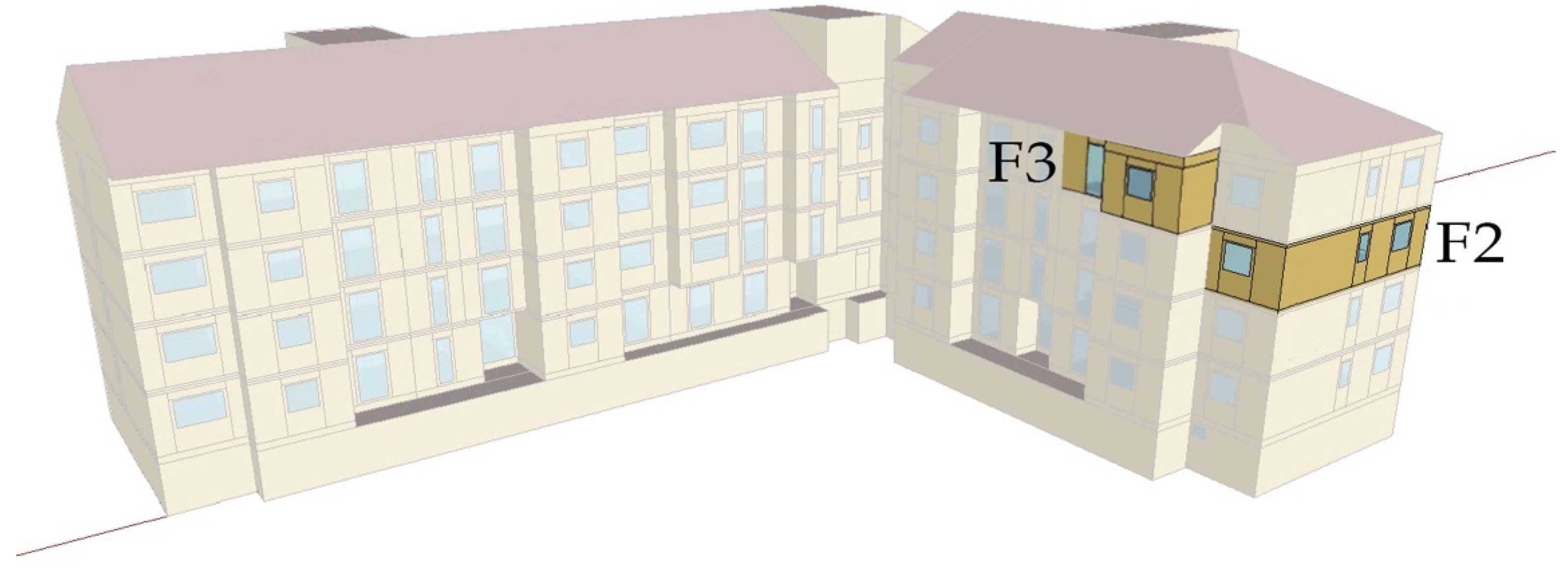
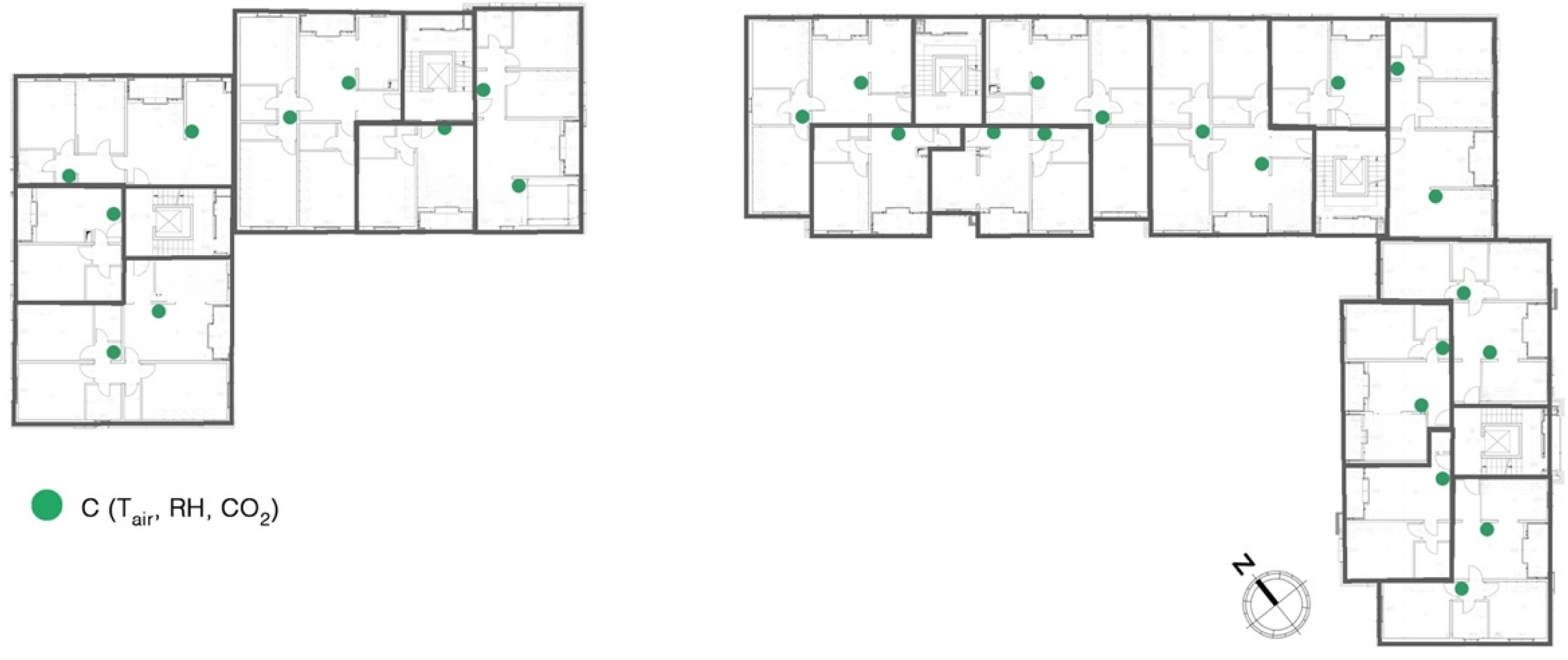
3.1. Description of the Building

The construction is a public social housing block built in 1980 consisting of two L-shaped buildings, named here Building 1 and Building 2 (described in Table 3), with four stories each and a total of 66 flats, and has recently been retrofitted (the installation of the façade insulation was completed in 2019, the thermal insulation of the slab separating the flats from the attic and the new windows were finalized in 2021).
The building envelope was made of prefabricated concrete elements, presenting almost no thermal insulation and with low-performance windows without appropriate solar shading (the installed roller blinds, very common in a large part of the building stock, simultaneously blocked radiation, daylight, and view, plus their container boxes created an important thermal bridge and were a source of air infiltration). The existing centralized heating system used fuel oil as the energy carrier, whereas each apartment was equipped with a local boiler for domestic hot water generation, using natural gas as the energy carrier. After the retrofit, natural gas remains in use only for cooking, while all the other energy uses rely on electrical energy, supplied by the national grid.
The retrofit strategy focused on the building envelope, aiming at a substantial reduction of the building’s “energy needs for heating and cooling” and providing, at the same time, adequate thermal comfort conditions for occupants. The opaque part of the building façade and the slab separating the flats from the uninhabitable attic were insulated with 0.25 m of mineral wool while the exposed ground floor slab was insulated with 0.10 m of phenolic resin. The existing windows were substituted with low-e double glazing windows and frames with thermal break. An exterior solar shading (motorized louvres manually operated by occupants) was installed on each window. The thermal bridge created by roller blinds was virtually eliminated by the elimination of the container box and a careful design of the integration of the new blinds and windows in the thermal envelope ensuring complete continuity of the insulation layer. The thermo-physical characteristics before and after the renovation are reported in Table 4.
In order to control heat losses due to ventilation, allowing at the same time for an adequate level of IAQ, a centralized mechanical ventilation system with heat recovery and by-pass (to allow for free cooling in summer and mid seasons) was installed, having an average specific fan power of 2.2 kW/(m3/s). However, the heat recovery is not yet working and currently the mechanical ventilation operates in extraction mode only. To verify the current extraction ventilation rate, a CO2 tracer gas method test (which evaluates the time of decay of the CO2 concentration) was carried out obtaining an average value of 0.13 ACH.
As a result of envelope improvement both in terms of thermal transmittance and air infiltration, and of the addition of heat recovery on ventilation, energy needs for heating are reduced to about 15 kWh/m2y as calculated with the semi stationary method adopted for Energy Performance Certification in Italy.
As for the active systems, high-performance centralized heating and DHW generation systems based on heat pumps were installed together with LED lamps for common areas lighting. The remaining final energy use will be partially complemented exploiting renewable energy source, i.e., a photovoltaic (PV) system for the production of electrical energy (127 m2 producing 19,800 kWh_electric/year) and a solar thermal system integrating the DHW system (20 m2 producing 9000 kWh_thermal/year).

3.2. Description of the Experiment: Flat Level

Two unoccupied flats were chosen for the experiment. They were heated to a targeted indoor operative temperature ranging from 24.5 °C (the upper comfort threshold) to 21.5 °C, using electric fan heaters of known electrical power (800 W or 1600 W depending on the size of the room). Their use allowed us to sharply control the start and finish of the delivery of thermal energy to the space. The switching on and off of these appliances (one per room, with bathrooms, lockers, and hallways excluded) took place remotely. The thermostatic function was performed via an air temperature sensor, placed in a barycentric position inside the apartment and far from the convective air flow generated by the electric air heaters. To obtain uniformity in temperature across the various rooms, we used ventilation fans to create air movement and mixing.
In some tests, the upper limit of comfort was exceeded in order for us to evaluate the impact of different initial temperatures of discharge and possible applications in buildings unoccupied during a certain period of the day or the week (e.g., offices).
All the windows and the main door were closed for the entire duration of the experiment while the external shading systems obscured about half of the opening, since it is not yet possible to dynamically manage their position even if they are motorized.
Both the apartments are located in Building 2 (see Table 3), on the second and third floor (see Figure 2). The flat on the second floor (F2) has a net floor area equal to 62 m2, exterior facing envelope area equal to 91 m2, and an S/V ratio of 0.44. It is characterized by an L shape: the living room and the kitchen are southeast facing, one bedroom and the bathroom are southwest oriented, and the second bedroom is northwest facing. The northeast side of the flat, where the kitchen is located, is facing towards the unheated staircase while the other two sides of the flat are adjacent to a flat which was unoccupied (and thus unheated) during the tests performed in the winter season 2021–2022. Above and under the flat there are other two occupied and heated apartments.
The flat on the third floor (F3) is rectangular and is entirely northwest facing. The net floor area is 41 m2, the exterior facing envelope area is 79 m2, and the S/V ratio is equal to 0.61. The corresponding flat located on the second floor was unheated and unoccupied during the tests performed in the winter season 2021–2022, the attic is unheated, and the separation slab was insulated (in 2021, before the start of the heating season).
The monitoring setup consists of sensors for measuring air temperature, surface temperature, and globe-thermometric temperature. Figure 3 shows the position of the sensors installed in the flat on the second floor, as an example. Table 5 provides the specification of the installed sensors. PT100 sensors were chosen to measure surface temperatures because they can better adhere to the surfaces.
In addition, sensors measuring air temperature were placed in the apartments adjacent to the flats under study, in the staircase, and in the attic to track the variation of temperature in the boundary environments.

3.3. Description of Demonstration Phase: Building Level

In each flat, sensors were installed to measure indoor air temperature prior to the beginning of the retrofit intervention. One-bedroom flats present one sensor, two or more rooms present two sensors. Figure 4 reports the floor type with the indication of the sensors’ localization, while Table 5 (code C) reports the sensors’ specifications.

4. Results

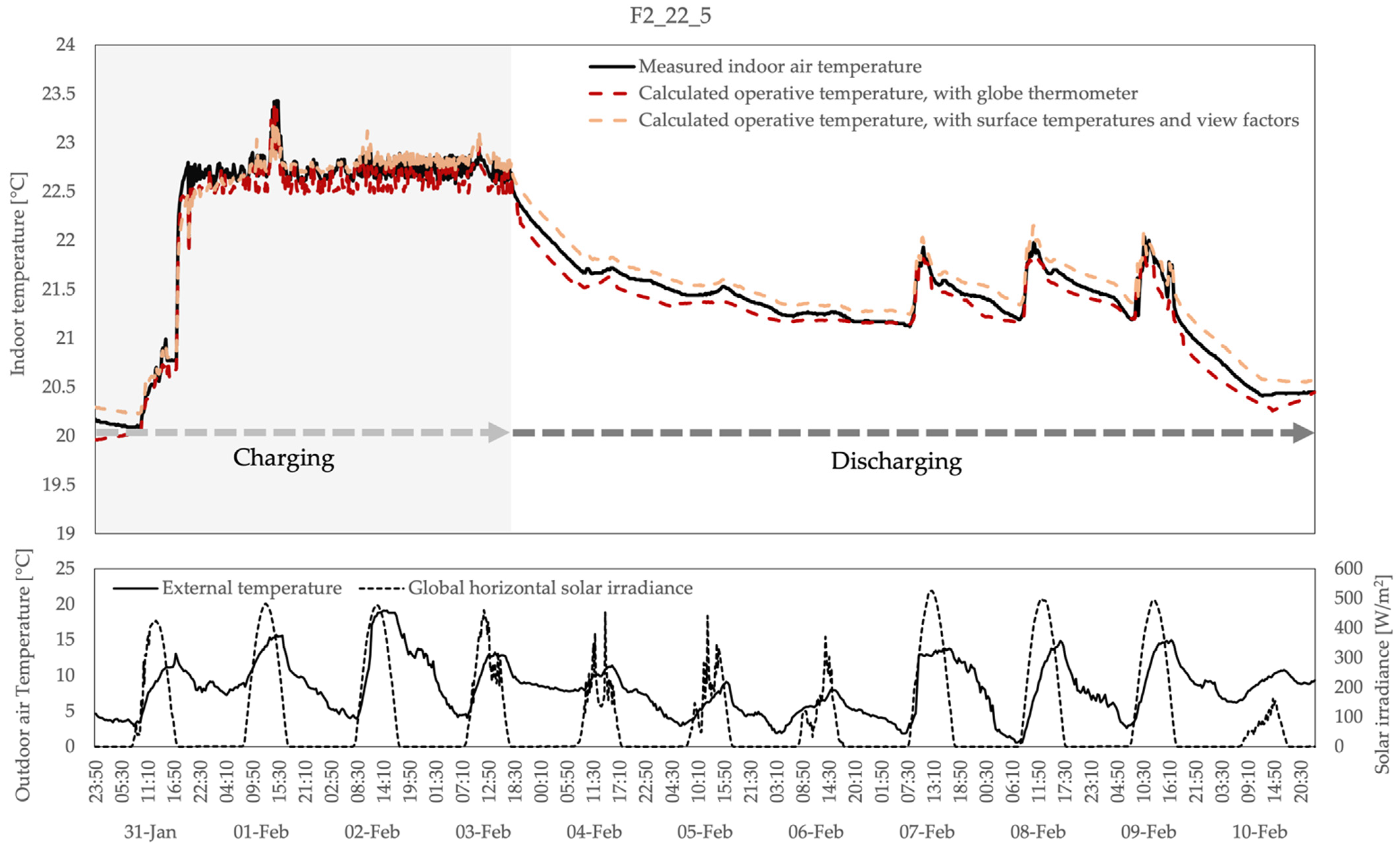
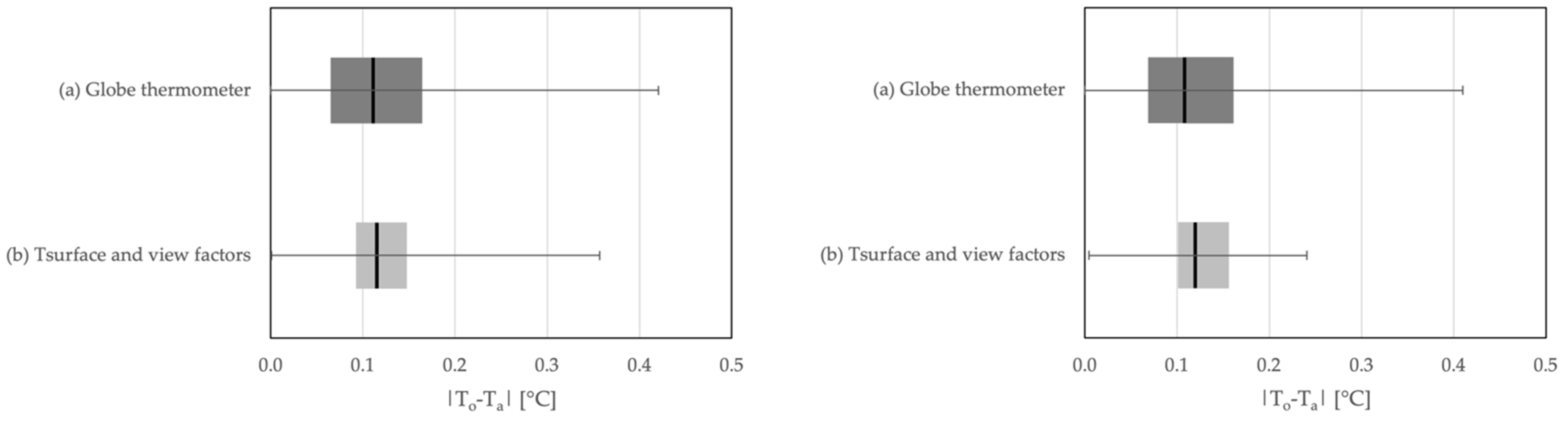
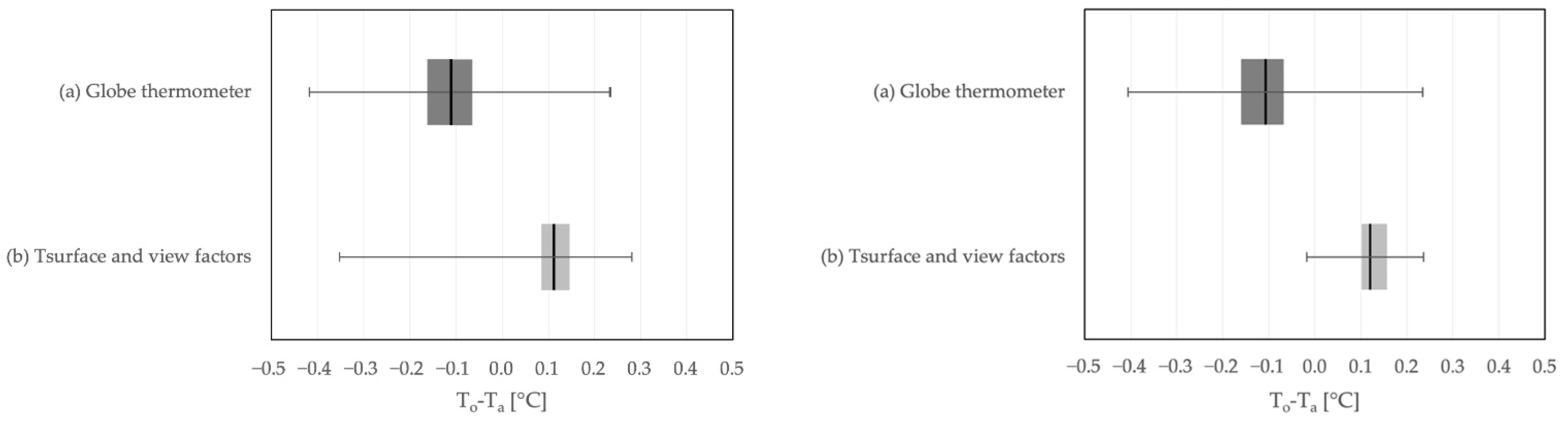
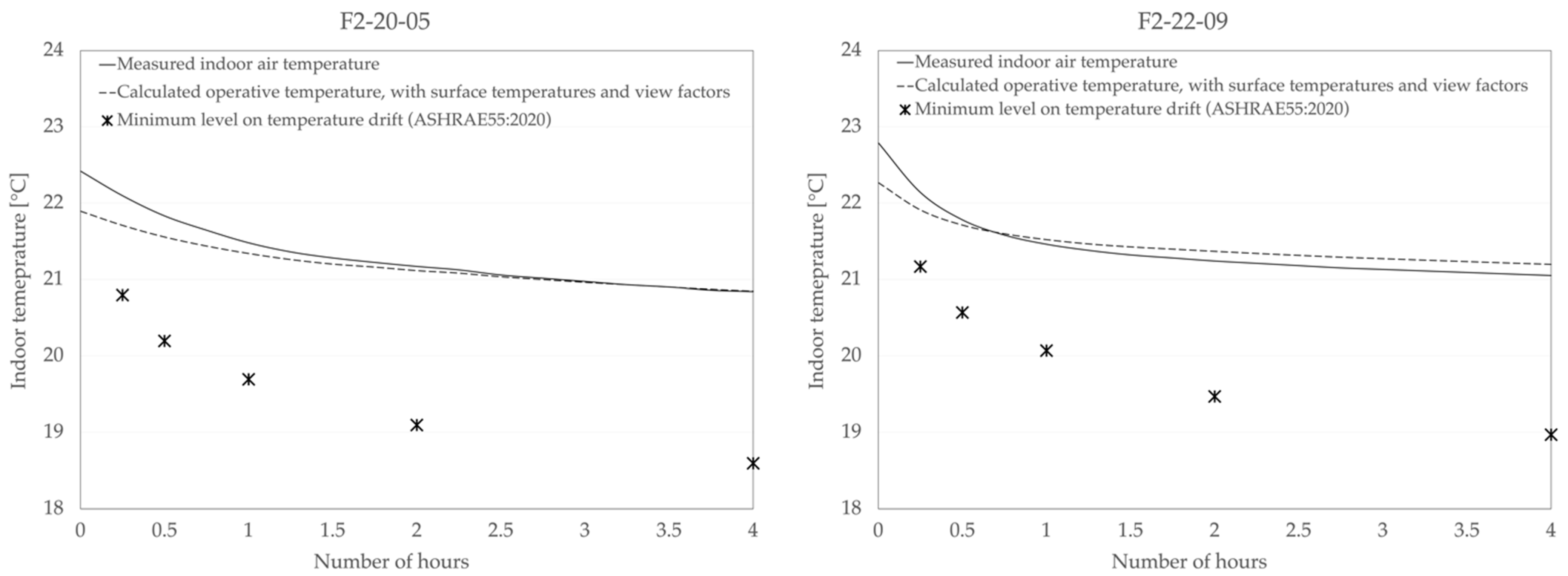
4.1. Comparison between Operative Temperature and Air Temperature

Figure 5 reports, as an example, one of the experimental tests realized during the heating season of 2021–2022 in the flat F2, described in Section 3.2. The three curves displayed in the figure represent, respectively, the operative temperature Top,g (calculated using a globe thermometer placed in the center of the room at the height of 1.7 m), the operative temperature Top,s (calculated from measured values of the temperature of the internal surfaces of the surrounding walls, their area, and their view factor between the chosen position in the room and the surfaces) and the measured air temperature Ta. The flexibility experiment is characterized by two stages: charge and discharge. In the charging phase, the three curves oscillate around the set-point temperature for a certain period of time to allow for the storage of thermal energy in the building structures. After switching off the heating system, the curves descend slowly, showing a slight difference between them. This similarity is found in all the conducted tests.
Overall, the three curves show a good response, allowing for the shift of the loads for more than 7 days during typical winter days in Milan characterized by an average air temperature of 7.8 °C (min 0.6 °C, max 15.0 °C) during the discharging phase, while maintaining adequate indoor comfort conditions.
Figure 6 and Figure 7 present the data distributions with box-and-whisker plots for the absolute and relative temperature differences, respectively, as described in Section 2.1. The boxes represent the interquartile range (i.e., 25th–75th percentiles) and the whiskers represent the minimum and the maximum. The median absolute value is 0.11 °C (0.00, 0.07, 0.16, 0.42 °C) when using the black-globe thermometer and 0.11 °C (0.00, 0.09, 0.14, 0.35 °C) considering the temperatures of the surrounding surfaces, in the case of the whole test. Focusing only on the discharge stage, they change, respectively, to 0.11 °C (0.00, 0.07, 0.16, 0.41 °C) and 0.12 °C (0.00, 0.10, 0.15, 0.24 °C). Considering the values reported in Table 5, it can be noted that the median absolute values are lower than the measurements’ uncertainty on air temperature (±0.2). The median relative value is −0.11 °C (−0.42, −0.16, −0.07, 0.23 °C) when using the black-globe thermometer and 0.11 °C (−0.35, 0.09, 0.14, 0.28 °C) considering the temperatures of the surrounding surfaces, in the case of the whole test. Focusing only on the discharge stage, they change, respectively, to −0.11 °C (−0.41, −0.16, −0.07, 0.23 °C) and 0.12 °C (−0.02, 0.10, 0.15, 0.24 °C).
On the basis of the analyses and as expected in constructions characterized by a well-insulated envelope, such as the building under study, the air temperature can be considered sufficiently representative of the operative temperature of the indoor environment, without a detrimental impact on thermal comfort analyses. Therefore, in the following we will display only air temperature.

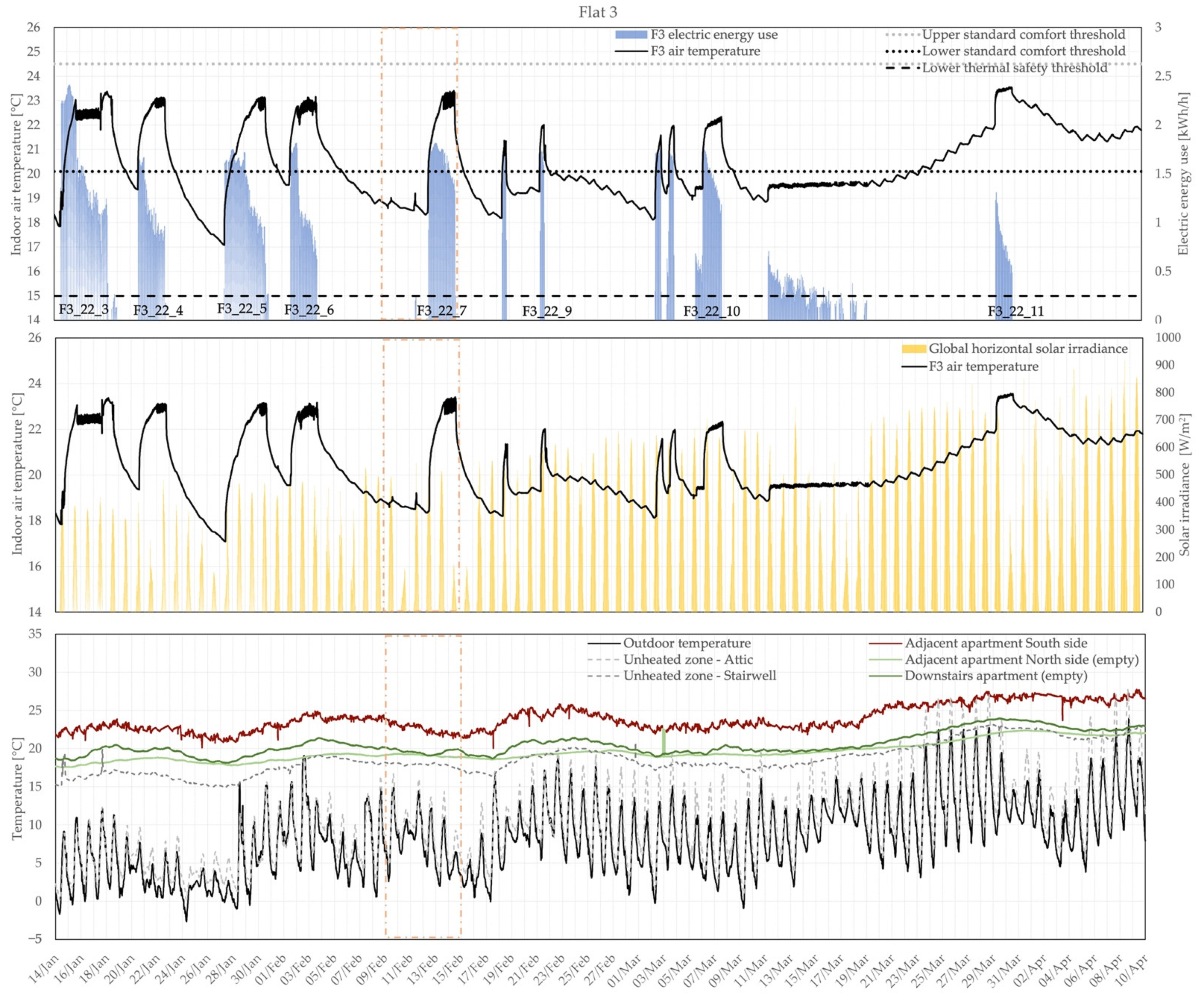
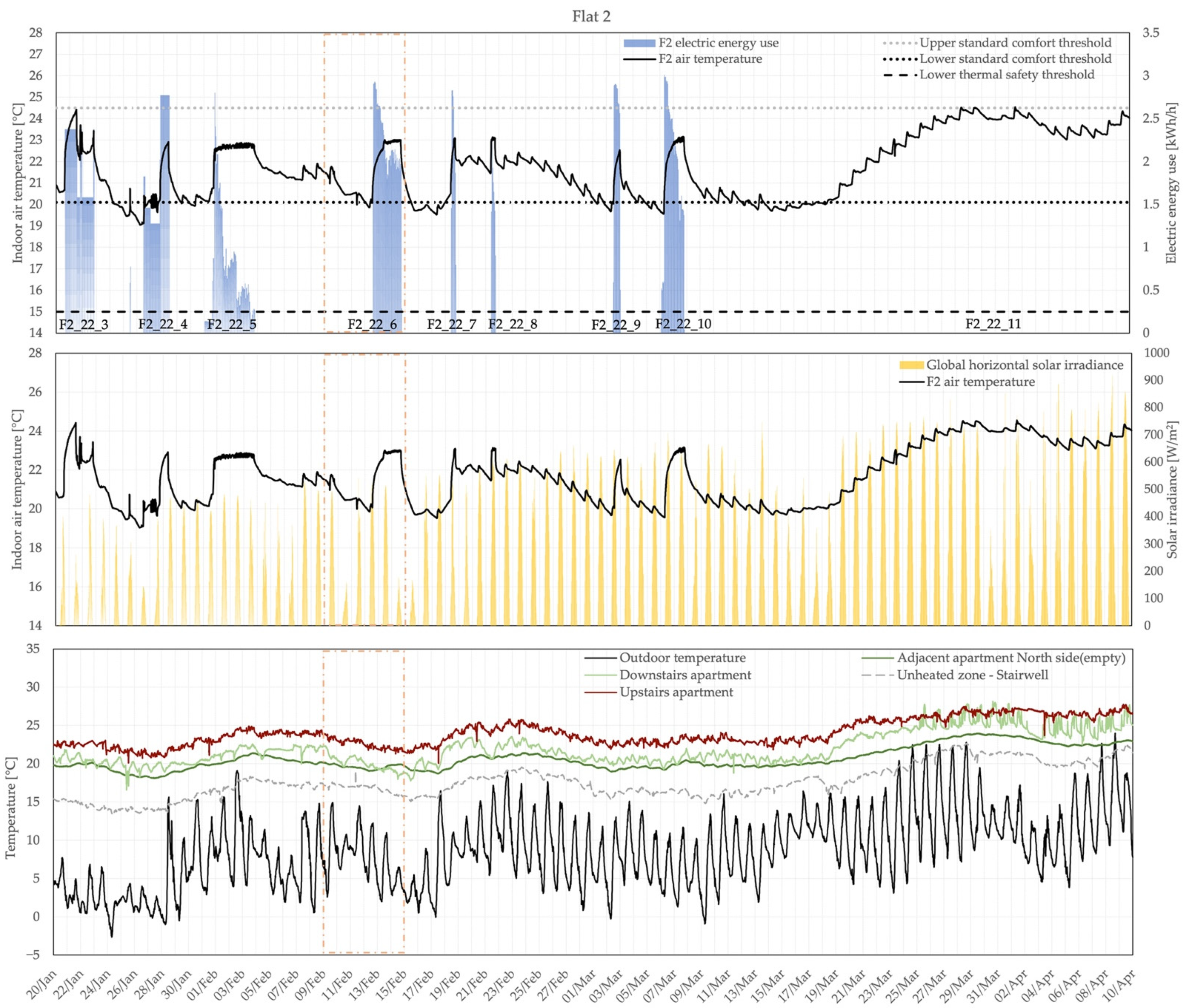
4.2. Assessment at the Flat Level

Around thirty experimental tests were conducted during the winter seasons of 2019/2020, 2020/2021, and 2021/2022 to evaluate the impact of different variables (orientation, duration of charging phase, initial temperature of discharge, outdoor weather conditions) on the energy flexibility potential given by the building’s thermal mass in an energy-retrofitted building. We interrupted the test when temperature dropped a few degrees below the lower limit of the comfort range or a few days after the interruption of the energy delivery even if the apartment was still in the comfort range (its full extension in the thermal safety zone has not been measured for practical reasons).
In all the tests, the rate of change in temperature during discharging does not exceed comfort acceptability limits, as indicated in ASHRAE 55 2020 [58] and reported in Table 2. Figure 8 shows two examples of verification of temperature drift.
Table 6 reports the list of the tests performed in the building and provides an overview of the main features: number of days of charging Δtc; duration in days of load-shifting (no active energy input) before temperature falls below the lower limit of the comfort range Δt EN 16798–1:2019 [54] and below the lower thermal safety limit (ΔtTS); initial temperature of discharge Ti; minimum temperature reached during the discharging phase Tmin; temperature drop ΔTAfter n days after 1, 2, and 3 days; and outdoor air temperature Tout (average, minimum and maximum) in degree Celsius.
Figure 9 and Figure 10 show the indoor air temperature variation in the flats F2 and F3, located, respectively, on the second floor and south oriented and on the third floor and north oriented. The figures focus on the tests conducted during the winter season 2021–2022 as they provide the most representative picture of the building’s behavior after the retrofit (the attic insulation and the installation of the windows were completed in 2021). It should be noted that F2 and F3 have quite different boundary conditions, which are reported, respectively, in Figure 9 and Figure 10. F2 is adjacent to an empty flat while the two apartments located on the lower and upper floor are occupied and heated. The remaining side is adjacent to the unheated stairs. F3 is adjacent to an occupied flat (south oriented) while the adjacent north-oriented one is not heated. Additionally, the flat below is unheated and the space above (attic), which is separated by a thermal insulated slab, shows temperatures very similar to the outdoor environment. During the tests, an unplanned thermal energy interruption (highlighted in figures in orange) took place from the 9 to 15 February 2022 in the whole building complex (except for the flats under study which were heated by local electrical heaters).
Both the flats show that the load can be shifted from some hours to several days while guaranteeing standard indoor comfortable conditions, depending on the period of precharging, the initial temperature of discharge, outdoor weather conditions, and thermal conditions of adjacent flats. The lower thermal safety limit is always respected in the tests.
In F2, the discharge is generally slower with respect to F3, and the curves show more obviously the impact of solar irradiance. F2 can shift the load from 17 h to up to 8 days, during typical winter days. The orientation and the proximity to the roof affect the indoor temperature conditions in F3, which, however, is able to maintain comfortable conditions from 9 h to up to 4 four days, during typical winter days. Both the flats are able to provide comfortable conditions without active energy input up to 11 days when the weather is milder (shoulder seasons). In both the flats, a load shifting of 17 h was registered in correspondence with the unplanned energy interruption which occurred in the whole housing complex. The length of the charging phase affects the results: a quick charge generally corresponds to a quicker drop in temperature. Furthermore, higher initial temperatures of discharge correspond to longer load shifts. Finally, the length of the discharging period varies on the base of the outdoor weather conditions: lower external temperatures correspond to shorter periods of thermal autonomy. The average duration is about 1 day for F2 and 1.5 days (37 h) for F3 when the average outdoor air temperatures is between 0 and 4 °C. For average outdoor air temperatures between 4 and 8 °C, the average length of comfort period is 4.8 days (115 h) for F2 and 2.1 days (52 h) for F3. When the average outdoor air temperature is between 8 and 12 °C during the discharge period, the average thermal autonomy of F2 remains equal to 4.8 days and increases to 3.5 (84 h) for F3.
The analyses of the tests on site are aligned with the results available in literature based on energy simulations [6,8], even if the large number of variables involved (thermo-physical properties of the building, period of charging, outdoor weather conditions, conditions of adjacent spaces, initial temperature of discharge, etc.) can significantly affect the outputs.

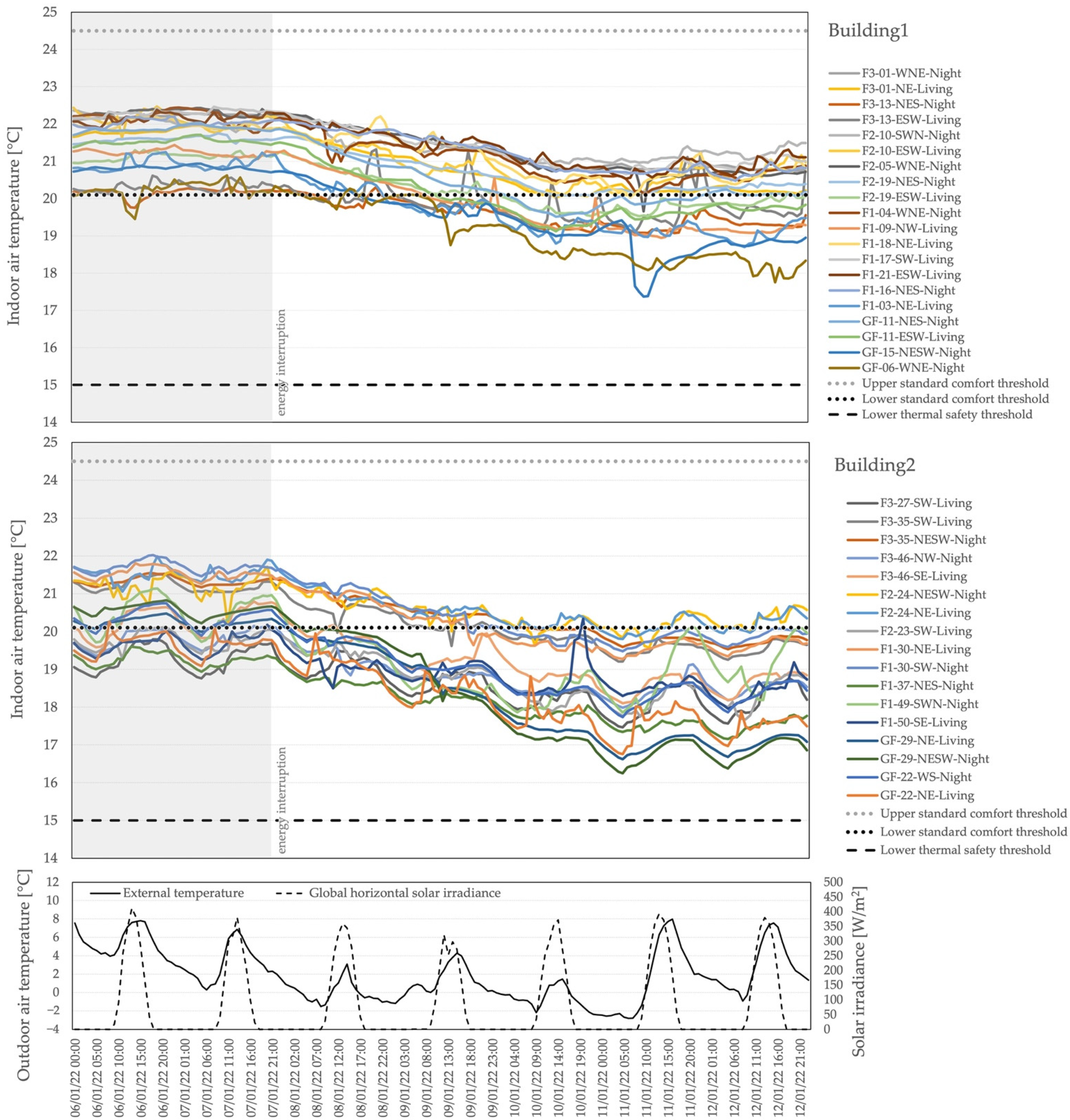
4.3. Assessment at the Entire Building Level

Figure 11 and Figure 12 show the indoor temperature evolution after the occurrence of unplanned energy interruptions, in the apartments of Building 1 and Building 2. Unoccupied flats were excluded from the analysis since they were unheated, and apartments where anomalies in data acquisition occurred were excluded as well. The legend allows one to identify the floor (GF = ground floor, F1/2/3 = first/second/third floor above the ground), the orientation of the apartment, and if the sensor is located in the living or night area.
The first energy interruption occurred on the 7 January 2022, at 10 p.m. (Figure 11) and lasted five days. Before that date, it is possible to notice that all the flats in Building 1 were within the standard thermal comfort range, even if a certain variability among the apartment can be observed due to orientation, solar and internal gains, occupant behavior, and preferences [59]. After the power outage, all the flats except the ones that showed the lowest indoor air temperature (20 °C) remained in comfort conditions for 54 h. Considering the thermal safety approach, all the apartments show an indoor air temperature higher than the ASHRAE winter survivability lower comfort threshold after 5 days. It is worth noting that generally, the flats located on the ground floor show the lowest indoor air temperatures and first reach the lower standard comfort limit. Despite different starting temperatures, the decay during the first two days is in the order of 1.5 °C for all the apartments.
In Building 2, the registered indoor air temperature before the energy interruption is generally lower with respect to Building 1 (half of the flats reported in Figure 11—Building 2 results are outside the comfort range even before the disruption event and only one flat registered a peak of 22 °C). After the outage, the flats which presented an indoor air temperature at least higher than 21 °C were able to maintain comfortable indoor conditions for at least 2 days. The apartments in which the indoor air temperature before the heating system shutdown was between 20 and 21 °C have reached the lower comfort limit after 7 h. Overall, the building survived above the thermal safety threshold for the whole duration of the system failure.
The second interruption occurred on the 9 February 2022 at 4 a.m. In this case, the system was reactivated after 30 h for around 1 day, but a second shutdown occurred on the 11 February at 10 a.m. After that, the two buildings remained without heating for 4 days.
In Building 1, before the energy interruption, all the flats except two were within comfort limits showing temperatures between 20 and 22 °C. After the first interruption, the majority of the flats remained in comfort conditions for 15 h. The reactivation of the heating system allowed for the slight increase of the indoor air temperatures of all the apartments. Before the second interruption, half of the flats presented an indoor air temperature between 21.5 °C and 20.1 °C. These flats remained in comfort from one to two days. All the flats were able to remain above the thermal safety limit for the whole duration of the power outage. It is worth noting that the north-oriented flats located at the lower levels are those which start the discharge from lower internal temperatures and undergo a sharper decrease (3.5 °C difference in 4 days). The south-oriented flats located on the upper floors register the highest values for the indoor air temperatures.
In Building 2, almost all the flats show indoor air temperatures within comfort limits before the first heating system failure. In the following 30 h, all the apartments maintained comfortable indoor conditions, except for the four flats which presented an indoor air temperature lower than the comfort limits even before the energy interruption. After the second outage, the flats which presented an indoor air temperature of 22 °C remained in comfort conditions for about 3 days; those that showed indoor air temperatures of 21 °C remained in comfort conditions for at least 2 days. Overall, the building was able to maintain conditions 2 °C higher than the thermal safety threshold for all the 4 days.
Figure 13 compares the thermal behavior of a sample flat after the power outage detailed in Figure 11 with the behavior of a flat in a high-energy-needs (poor thermal envelope) building, which well represents the case study in the pre-retrofit conditions. Specifically, apartment F1-03-NE (facing northeast) was selected for the low-energy-needs building, while an east-oriented flat in a multistory residential building located in Milan was chosen to represent the high-energy-needs building. The low-energy-needs building remained in comfort after the energy interruption for about 1 day and never exceeds the thermal safety threshold for the entire power outage period, reaching a minimum temperature of 18.7 °C. The high-energy-needs building has an autonomy of 2.5 h within the lower standard comfort threshold and 2.5 days before reaching the lower thermal safety limit. The effectiveness of the retrofit measures is evident from the extension of the period of time in which the low-energy-needs building remains in comfort and the thermal safety conditions.

5. Discussion and Further Research

The paper explores and provides evidence of some additional benefits provided by a deep energy retrofit, which are rarely taken into account or known by building users and many stakeholders, as highlighted by the Open Public Consultation on the Renovation Wave [19]. In particular, it evaluates and demonstrates the potential for deeply retrofitted buildings to act as thermal batteries while providing adequate indoor comfort conditions. It focuses the analyses on a residential public building, which should serve as a role model and reference point for documenting and communicating to building users and owners, with high quality data, the extent of the flexibility gained, and a sound basis for setting up flexibility strategies which can be helpful for energy operators and building managers. In fact, the energy flexibility provided by the thermal mass of the building can be exploited for demand-side flexibility actions and can bring several benefits: enhanced possibilities of self-use of locally generated renewable energy, reduction of demand in coincidence with system peaks, adaptation to climate change, and more frequent and violent extreme weather events.
The results presented in Section 4.2 and Section 4.3 allow one to verify through measurements that an increased external thermal insulation of walls, roofs, and basements; strong reduction of thermal bridges; new glazings; and frames with good thermal and air tightness features can considerably extend the time interval during which a building will maintain indoor conditions in the comfort range without any active supply of energy with respect to a high-energy-needs building, as suggested by, e.g., the following studies based on energy simulations: [6,8,42,43]. The load-shifting period depends on a series of factors such as the duration of charging, the initial temperature of discharge, the outdoor weather, the thermal conditions of the adjacent environment, and the orientation. In particular, the tests confirm that apartments which can exploit solar energy gains better than others thanks to better exposure to sun radiation are positively affected with respect to the time interval during which adequate comfort conditions are maintained after turning off the heating system. For the south-oriented apartment (F2), the achievable load-shifting period goes from 17 h up to 8 days, while in the northwest-oriented flat (F3) the load-shifts can vary from 9 h to 4 days.
Moreover, the demonstration phase in Section 4.3 points out that the flats located on the lower floor (and having hence a larger exposed surface, since the building is on pilotis) have generally lower temperatures with respect to the ones located on the upper floors, and this also affects the possibility of remaining in comfortable conditions after an energy interruption. However, the study allows one to verify that all the apartments of the retrofitted buildings are able to maintain habitable indoor conditions under extreme events, such as a power outage [57], for at least 5 days [41,44].
Finally, Section 4.1 adds further evidence to the fact that in deep retrofitted buildings, the operative temperature and air temperature are actually very close to each other, and this allows one to simplify the measurements on site considering just air temperature sensors. Furthermore, this means that the reduction of thermal transmittance for the opaque and transparent envelope’s elements and the correction of thermal bridges in energy retrofits allow one to obtain very uniform surface temperatures, increasing comfort and occupants’ acceptance in every part of the building, including the periphery, rising the value of the building. Before the retrofit, in fact, a number of occupants were complaining about thermal discomfort and the formation of molds on cold parts of surfaces. To estimate this increased value, it can be observed that in a well-made retrofitted building, 100% of the (economically valuable) space is perfectly in comfort, while in a pre-retrofit building, a certain portion of the floor space would not be in comfort, e.g., due to surfaces with too high or too low temperatures, lack of or incorrect control of solar protections, etc.
This paper fills a gap in the literature by providing measured data to assess the flexibility potential given by the thermal mass in retrofits that highly reduce thermal losses. The results of this research are obviously, for some aspects, specific to the analyzed case study, but the chosen building typology is quite common in Italy (and other parts of EU) and hence, results can be extended to a significant fraction of the building stock. Furthermore, the methodology and the developed experimental setup can be used to assess the increase in flexibility which can be obtained by deep retrofitting other building typologies, thus analyzing the possibility to create building portfolios which allow one to set up flexibility services at the district scale.
The investigations were carried out under average winter weather conditions, typically registered in Northern Italy and more generally in areas characterized by a humid subtropical climate (Koppen climate classification) with the coldest month averaging above 0 °C. Other types of climatic conditions will be taken into account through studies based on energy simulations in future works.
Future research will also investigate the effects of different variables (e.g., presence of occupants, activation of the mechanical ventilation with heat recovery, presence of furniture, etc.) through the use of simulation models calibrated to make use of the dataset of measurements presented and analyzed in this paper.
The models will be used to assess different strategies to store renewable energy via short-term load shifting (e.g., to cope with the daily cycle of PV and short disruptions due to passing clouds) or longer shifts (e.g., under variations on the time scale of days/weeks in the outputs of renewable sources as a result of weather variability) and to cope with extreme weather events. Moreover, following a similar approach, tests and measurements will be carried out during the cooling season, which is currently the less investigated season in literature when analyzing flexibility.
Future studies will also extend the investigation to assess the technical feasibility in relation to the installed energy service systems and the control of the energy demand in the building. Another important aspect will be the evaluation of the economical effectiveness and the users’ motivation and acceptability of the proposed solution to analyze the possibility to deliver flexibility services to both the occupants and the grid.

6. Conclusions

This study, based on measured data presented in this paper, explores the role of deep retrofitted buildings in acting as thermal batteries able to enhance the possibility of self-consumption of locally generated renewable energy, provide energy flexibility services to the energy system, and protect occupants from the effects of large energy interruptions. The analyses are based on the data registered in around thirty experimental tests in two unoccupied flats of a multiapartment building, realized during the winter season and on two unplanned heating power outages which involved the entire building complex.
High quality renovation of existing buildings, in particular with high insulation levels of the external envelope, careful reduction/elimination of thermal bridges, and improved air tightness and heat recovery on ventilation can reduce the “energy need for heating” of existing buildings by up to 80–90%, down to 15–30 kWh/m2y [22]. This low level of energy needs might be a key to accelerate the decarbonization of supply and bring it to a sufficient pace to substitute fossil fuels and maintain the carbon budget trajectory below what is needed for keeping 50% probability of limiting global warming to 1.5 °C [60]. Low levels of energy needs, by limiting the size of infrastructure for capturing, transporting, and storing renewable energy, might both ease deploying the, thus reduced, capital investments and favor social acceptance of the, thus reduced, land-take in the territories.
However, as shown by measurements in the presented case study, the large reduction of energy needs achievable by deep renovation has other important effects. By making the thermal energy demand of buildings much more flexible, deep retrofit might be essential for allowing the massive electrification of thermal end-uses without creating the need for the large, new capacity installation to cope with peak demand, which would be necessary under the present situation of the building stock or under a mild renovation scenario.
By extending to a few days, rather than a few hours, the time under which a building can remain in the thermal comfort range, deep renovations might be essential for making buildings much safer under the disruptions of energy supply whose probability is rising with the increased likelihood of extreme weather events. The presented analysis brings the availability of data measured in a case study on the above flexibility, adding empirical data to several recent papers exploring flexibility mainly via simulation, as reported in the literature review.
Future work planned in the context of the H2020 project SATO is the development of energy flexibility services to be offered to managers of building portfolios (such as social housing companies) or other aggregated groups of buildings, energy companies, or system operators engaged in delivering stable energy system operations and services in a scenario of rapid entrance of intermittent renewables and of growing risk of extreme weather events. The living laboratories of the retrofitted buildings analyzed in this paper will be used as a test ground for some of the flexibility services and for the users’ motivation and acceptance of the proposed solutions.

Author Contributions

Conceptualization, S.E.; methodology, S.E.; investigation, S.E. and A.B.; data curation, S.E. and A.B.; formal analysis, S.E. and A.B.; software, S.E.; writing—original draft preparation, S.E.; writing—review and editing, S.E. and A.B.; visualization, S.E. and A.B.; funding acquisition, S.E. All authors have read and agreed to the published version of the manuscript.

Funding

The study was partly developed within the framework of the project SATO (Self Assessment Towards Optimization of Building Energy), which has received funding from the European Union’s Horizon 2020 research and innovation program under grant agreement No. 957128 and partly supported by a grant by INPS (Istituto Nazionale Previdenza Sociale) for research entitled “Highly insulated building fabric as thermal storage for renewable energy and flexible elements necessary for future smart cities”.

Data Availability Statement

The data presented in this study will be available in “Measured indoor environmental data in a retrofitted multiapartment building to assess energy flexibility and thermal safety during winter power outages”, under submission to data journal.

Acknowledgments

We acknowledge the support in data collection received from S. Bardeschi and F. Manzoni of Municipality of Milano, and R. Armani and A. Sangalli of Politecnico di Milano.

Conflicts of Interest

The authors declare no conflict of interest.

Abbreviations

The following abbreviations are used in this manuscript:
GsGlobal horizontal Solar irradiance [W/m2]
MRTMean Radiant Temperature [°C]
MRTgCalculated mean radiant temperature with globe thermometer in a specified point [°C]
MRTsCalculated mean radiant temperature with surface temperatures and view factors calculated from a specified point [°C]
RESRenewable Energy Sources
TaMeasured indoor air temperature [°C]
Ta,adjMeasured indoor air temperature of adjacent apartment [°C]
Ta,atticMeasured indoor air temperature of unoccupied attic [°C]
Ta,outMeasured outdoor air temperature [°C]
Ta,stairMeasured stairwell air temperature [°C]
TiInitial temperature of discharge [°C]
TminMinimum temperature reached during the discharging phase [°C]
ΔTAfter 1 dayTemperature drop after 1 day of discharge [°C]
ΔTAfter 2 daysTemperature drop after 2 days of discharge [°C]
ΔTAfter 3 daysTemperature drop after 3 days of discharge [°C]
Tout Avg (min; max)Outdoor air temperature (average, minimum and maximum) [°C]
TESThermal energy storage
ToOperative temperature
Top,gCalculated operative temperature with globe thermometer in a specified point [°C]
Top,sCalculated operative temperature with surface temperatures and view factors calculated from a specified point [°C]
ΔtcNumber of days of charging [days]
Δt EN 16798-1:2019Duration of load-shifting (no active energy input) before temperature falls below the lower limit of the comfort range [days]
Δt TSDuration of load-shifting (no active energy input) before temperature falls below the lower thermal safety limit [days]

References

  1. Koohi-Fayegh, S.; Rosen, M.A. A review of energy storage types, applications and recent developments. J. Energy Storage 2020, 27, 101047. [Google Scholar] [CrossRef]
  2. Arteconi, A.; Hewitt, N.J.; Polonara, F. State of the art of thermal storage for demand-side management. Appl. Energy 2012, 93, 371–389. [Google Scholar] [CrossRef]
  3. Heier, J.; Bales, C.; Martin, V. Combining thermal energy storage with buildings—A review. Renew. Sustain. Energy Rev. 2015, 42, 1305–1325. [Google Scholar] [CrossRef]
  4. Sarbu, I.; Sebarchievici, C. A Comprehensive Review of Thermal Energy Storage. Sustainability 2018, 10, 191. [Google Scholar] [CrossRef] [Green Version]
  5. Jensen, S.Ø.; Marszal-Pomianowska, A.; Lollini, R.; Pasut, W.; Knotzer, A.; Engelmann, P.; Stafford, A.; Reynders, G. IEA EBC Annex 67 Energy Flexible Buildings. Energy Build. 2017, 155, 25–34. [Google Scholar] [CrossRef] [Green Version]
  6. Foteinaki, K.; Li, R.; Heller, A.; Rode, C. Heating system energy flexibility of low-energy residential buildings. Energy Build. 2018, 180, 95–108. [Google Scholar] [CrossRef]
  7. Johra, H.; Heiselberg, P.; Dréau, J.L. Influence of envelope, structural thermal mass and indoor content on the building heating energy flexibility. Energy Build. 2019, 183, 325–339. [Google Scholar] [CrossRef]
  8. Le Dreau, J.; Heiselberg, P. Energy flexibility of residential buildings using short term heat storage in the thermal mass. Energy 2016, 111, 991–1002. [Google Scholar] [CrossRef]
  9. Oliveira Panão, M.J.N.; Mateus, N.M.; Carrilho da Graça, G. Measured and modeled performance of internal mass as a thermal energy battery for energy flexible residential buildings. Appl. Energy 2019, 239, 252–267. [Google Scholar] [CrossRef]
  10. Wijesuriya, S.; Booten, C.; Bianchi, M.V.; Kishore, R.A. Building energy efficiency and load flexibility optimization using phase change materials under futuristic grid scenario. J. Clean. Prod. 2022, 339, 130561. [Google Scholar] [CrossRef]
  11. Johra, H.; Heiselberg, P. Influence of internal thermal mass on the indoor thermal dynamics and integration of phase change materials in furniture for building energy storage: A review. Renew. Sustain. Energy Rev. 2017, 69, 19–32. [Google Scholar] [CrossRef]
  12. Balint, A.; Kazmi, H. Determinants of energy flexibility in residential hot water systems. Energy Build. 2019, 188–189, 286–296. [Google Scholar] [CrossRef]
  13. D’Ettorre, F.; De Rosa, M.; Conti, P.; Testi, D.; Finn, D. Mapping the energy flexibility potential of single buildings equipped with optimally-controlled heat pump, gas boilers and thermal storage. Sustain. Cities Soc. 2019, 50, 101689. [Google Scholar] [CrossRef]
  14. Chen, Y.; Xu, P.; Chen, Z.; Wang, H.; Sha, H.; Ji, Y.; Zhang, Y.; Dou, Q.; Wang, S. Experimental investigation of demand response potential of buildings: Combined passive thermal mass and active storage. Appl. Energy 2020, 280, 115956. [Google Scholar] [CrossRef]
  15. Stinner, S.; Huchtemann, K.; Müller, D. Quantifying the operational flexibility of building energy systems with thermal energy storages. Appl. Energy 2016, 181, 140–154. [Google Scholar] [CrossRef]
  16. Reynders, G.; Amaral Lopes, R.; Marszal-Pomianowska, A.; Aelenei, D.; Martins, J.; Saelens, D. Energy flexible buildings: An evaluation of definitions and quantification methodologies applied to thermal storage. Energy Build. 2018, 166, 372–390. [Google Scholar] [CrossRef]
  17. Attia, S.; Levinson, R.; Ndongo, E.; Holzer, P.; Berk Kazanci, O.; Homaei, S.; Zhang, C.; Olesen, B.W.; Qi, D.; Hamdy, M.; et al. Resilient cooling of buildings to protect against heat waves and power outages: Key concepts and definition. Energy Build. 2021, 239, 110869. [Google Scholar] [CrossRef]
  18. European Commission. A Renovation Wave for Europe—Greening our Buildings, Creating Jobs, Improving Lives. 2020. Available online: https://eur-lex.europa.eu/legal-content/EN/TXT/PDF/?uri=CELEX:52020DC0662&from=EN (accessed on 8 June 2022).
  19. European Commission Stakeholder Consultation on the Renovation Wave Initiative. Synthesis Report. 2020. Available online: https://energy.ec.europa.eu/system/files/2020-10/stakeholder_consultation_on_the_renovation_wave_initiative_0.pdf (accessed on 8 June 2022).
  20. Monteiro, C.S.; Causone, F.; Cunha, S.; Pina, A.; Erba, S. Addressing the challenges of public housing retrofits. Energy Procedia 2017, 134, 442–451. [Google Scholar] [CrossRef]
  21. Shnapp, S.; Sitjà, R.; Laustsen, J. What is a Deep Renovation Definition? 2013. Available online: https://www.gbpn.org/wp-content/uploads/2021/06/08.DR_TechRep.low_.pdf (accessed on 8 June 2022).
  22. Erba, S.; Pagliano, L. Combining Sufficiency, Efficiency and Flexibility to Achieve Positive Energy Districts Targets. Energies 2021, 14, 4697. [Google Scholar] [CrossRef]
  23. White, L.M.; Wright, G.S. Assessing Resiliency and Passive Survivability in Multifamily Buildings; ASHARE: Atlanta, GA, USA, 2019; pp. 123–134. [Google Scholar]
  24. Intergovernmental Panel on Climate Change IPCC. Climate Change 2021: The Physical Science Basis. In Contribution of Working Group I to the Sixth Assessment Report of the Intergovernmental Panel on Climate Change; Masson-Delmotte, V., Zhai, P., Pirani, A., Connors, S.L., Péan, C., Berger, S., Caud, N., Chen, Y., Goldfarb, L., Gomis, M.I., et al., Eds.; Cambridge University Press: Cambridge, UK; New York, NY, USA, 2021. [Google Scholar]
  25. Passive Survivability and Back-Up Power During Disruptions|U.S. Green Building Council. Available online: https://www.usgbc.org/credits/passivesurvivability (accessed on 22 May 2021).
  26. RELi Rating Guidelines for RESILIENT DESIGN + CONSTRUCTION. U.S. GREEN BUILDING COUNCIL. 2020. Available online: https://www.usgbc.org/resources/reli-20-rating-guidelines-resilient-design-and-construction (accessed on 8 June 2022).
  27. Decreto del Presidente della Repubblica D.P.R. 26 August 1993, n.412—Regolamento Recante Norme Per la Progettazione, L’installazione, L’esercizio e la Manutenzione Degli Impianti Termici Degli Edifici ai Fini del Contenimento dei Consumi di Energia, in Attuazione Dell’art. 4, Comma 4, della Legge 9 Gennaio 1991, n. 10. 1993. Available online: https://www.gazzettaufficiale.it/eli/id/1993/10/14/093G0451/sg (accessed on 8 June 2022).
  28. De Rosa, M.; Bianco, V.; Scarpa, F.; Tagliafico, L.A. Historical trends and current state of heating and cooling degree days in Italy. Energy Convers. Manag. 2015, 90, 323–335. [Google Scholar] [CrossRef]
  29. Morris, F.B.; Braun, J.E.; Treado, S.J. Experimental and simulated performance of optimal control of building thermal storage. ASHRAE Trans. 1994, 100, 402–414. [Google Scholar]
  30. Reynders, G.; Nuytten, T.; Saelens, D. Potential of structural thermal mass for demand-side management in dwellings. Build. Environ. 2013, 64, 187–199. [Google Scholar] [CrossRef]
  31. Vivian, J.; Chiodarelli, U.; Emmi, G.; Zarrella, A. A sensitivity analysis on the heating and cooling energy flexibility of residential buildings. Sustain. Cities Soc. 2020, 52, 101815. [Google Scholar] [CrossRef]
  32. Foteinaki, K.; Li, R.; Péan, T.; Rode, C.; Salom, J. Evaluation of energy flexibility of low-energy residential buildings connected to district heating. Energy Build. 2020, 213, 109804. [Google Scholar] [CrossRef]
  33. Kuczyński, T.; Staszczuk, A. Experimental study of the influence of thermal mass on thermal comfort and cooling energy demand in residential buildings. Energy 2020, 195, 116984. [Google Scholar] [CrossRef]
  34. Orosa, J.; Oliveira, A. A field study on building inertia and its effects on indoor thermal environment. Renew. Energy 2012, 37, 89–96. [Google Scholar] [CrossRef]
  35. Kensby, J.; Trüschel, A.; Dalenbäck, J.-O. Potential of residential buildings as thermal energy storage in district heating systems—Results from a pilot test. Appl. Energy 2015, 137, 773–781. [Google Scholar] [CrossRef]
  36. Lu, F.; Yu, Z.; Zou, Y.; Yang, X. Cooling system energy flexibility of a nearly zero-energy office building using building thermal mass: Potential evaluation and parametric analysis. Energy Build. 2021, 236, 110763. [Google Scholar] [CrossRef]
  37. Hu, M.; Xiao, F.; Jørgensen, J.B.; Li, R. Price-responsive model predictive control of floor heating systems for demand response using building thermal mass. Appl. Therm. Eng. 2019, 153, 316–329. [Google Scholar] [CrossRef]
  38. Liu, M.; Heiselberg, P. Energy flexibility of a nearly zero-energy building with weather predictive control on a convective building energy system and evaluated with different metrics. Appl. Energy 2019, 233–234, 764–775. [Google Scholar] [CrossRef]
  39. Reynders, G.; Diriken, J.; Saelens, D. Generic characterization method for energy flexibility: Applied to structural thermal storage in residential buildings. Appl. Energy 2017, 198, 192–202. [Google Scholar] [CrossRef] [Green Version]
  40. Zhang, C.; Kazanci, O.B.; Levinson, R.; Heiselberg, P.; Olesen, B.W.; Chiesa, G.; Sodagar, B.; Ai, Z.; Selkowitz, S.; Zinzi, M.; et al. Resilient cooling strategies—A critical review and qualitative assessment. Energy Build. 2021, 251, 111312. [Google Scholar] [CrossRef]
  41. Homaei, S.; Hamdy, M. Quantification of Energy Flexibility and Survivability of All-Electric Buildings with Cost-Effective Battery Size: Methodology and Indexes. Energies 2021, 14, 2787. [Google Scholar] [CrossRef]
  42. Wilson, A. Passive Survivability. In Climate Adaptation and Resilience Across Scales; Routledge: New York, NY, USA, 2021; pp. 141–152. ISBN 978-1-00-303072-0. [Google Scholar] [CrossRef]
  43. Urban Green Council. Baby It’s Cold Inside. Available online: https://www.urbangreencouncil.org/babyitscoldinside (accessed on 1 April 2022).
  44. Ozkan, A.; Kesik, T.; Yilmaz, A.Z.; O’Brien, W. Development and visualization of time-based building energy performance metrics. Build. Res. Inf. 2019, 47, 493–517. [Google Scholar] [CrossRef]
  45. Wolisz, H.; Harb, H.; Matthes, P.; Streblow, R.; Müller, D. Dynamic simulation of thermal capacity and charging/discharging performance for sensible heat storage in building wall mass. In Proceedings of the 13th Conference of International Building Performance Simulation Association, Chambéry, France, 26–28 August 2013; pp. 2716–2723. [Google Scholar]
  46. Chen, Y.; Chen, Z.; Xu, P.; Li, W.; Sha, H.; Yang, Z.; Li, G.; Hu, C. Quantification of electricity flexibility in demand response: Office building case study. Energy 2019, 188, 116054. [Google Scholar] [CrossRef]
  47. Weiß, T.; Fulterer, A.M.; Knotzer, A. Energy flexibility of domestic thermal loads—A building typology approach of the residential building stock in Austria. Adv. Build. Energy Res. 2019, 13, 122–137. [Google Scholar] [CrossRef]
  48. Vivian, J.; Chiodarelli, U.; Emmi, G.; Zarrella, A. Analysis of the Energy Flexibility of Residential Buildings in the Heating and Cooling Season; International Building Performance Simulation Association: Rome, Italy, 2019; pp. 270–277. [Google Scholar]
  49. Christensen, M.H.; Li, R.; Pinson, P. Demand side management of heat in smart homes: Living-lab experiments. Energy 2020, 195, 116993. [Google Scholar] [CrossRef]
  50. Tantawi, M.Z. Assessing Energy Flexibility Using a Building’s Thermal Mass as Heat Storage; Eindhoven University of Technology Research Portal: Eindhoven, The Netherlands, 2020. [Google Scholar]
  51. Zhang, X.; Gao, W.; Li, Y.; Wang, Z.; Ushifusa, Y.; Ruan, Y. Operational performance and load flexibility analysis of japanese zero energy house. Int. J. Environ. Res. Public Health 2021, 18, 6782. [Google Scholar] [CrossRef]
  52. Lu, F.; Yu, Z.; Zou, Y.; Yang, X. Energy flexibility assessment of a zero-energy office building with building thermal mass in short-term demand-side management. J. Build. Eng. 2022, 50, 104214. [Google Scholar] [CrossRef]
  53. Ding, Y.; Lyu, Y.; Lu, S.; Wang, R. Load shifting potential assessment of building thermal storage performance for building design. Energy 2022, 243, 123036. [Google Scholar] [CrossRef]
  54. EN 16798-1:2019; Energy Performance of Buildings-Ventilation for Buildings—Part 1: Indoor Environmental Input Parameters for Design and Assessment of Energy Performance of Buildings Addressing Indoor Air Quality, Thermal Environment, Lighting and Acoustics-Module M1-6. CEN-CENELEC Management Centre: Rue de la Science, Brussels, 2019.
  55. ISO EN ISO 7726:2001; Ergonomics of the Thermal Environment—Instruments for Measuring Physical Quantities. International Organization for Standardization: Geneva, Switzerland, 2001; p. 63.
  56. Tartarini, F.; Schiavon, S.; Cheung, T.; Hoyt, T. CBE Thermal Comfort Tool: Online tool for thermal comfort calculations and visualizations. SoftwareX 2020, 12, 100563. [Google Scholar] [CrossRef]
  57. ASHRAE Transactions—2016 Winter Conference—Orlando, FL Volume 122, Part 1. Available online: https://www.techstreet.com/standards/ashrae-transactions-2016-winter-conference-orlando-fl-vol-122-part-1?product_id=1914973 (accessed on 1 April 2022).
  58. ANSI/ASHRAE Standard 55-2020; Thermal Environmental Conditions for Human Occupancy. ASHARE: Peachtree Corners, GA, USA, 2020; p. 80.
  59. Salvia, G.; Morello, E.; Rotondo, F.; Sangalli, A.; Causone, F.; Erba, S.; Pagliano, L. Performance Gap and Occupant Behavior in Building Retrofit: Focus on Dynamics of Change and Continuity in the Practice of Indoor Heating. Sustainability 2020, 12, 5820. [Google Scholar] [CrossRef]
  60. Jackson, R.B.; Le Quéré, C.; Andrew, R.M.; Canadell, J.G.; Korsbakken, J.I.; Liu, Z.; Peters, G.P.; Zheng, B. Global energy growth is outpacing decarbonization. Environ. Res. Lett. 2018, 13, 120401. [Google Scholar] [CrossRef]
Figure 1. Methodology to assess the potential to deliver “long-term” flexibility in a deeply retrofitted multiapartment building with high thermal mass.
Energies 15 04405 g001
Figure 2. A 3D geometric model of the building highlighting the flat located on the second floor (F2) and the flat on the third floor (F3).
Energies 15 04405 g002
Figure 3. Position of sensors in the flat F2, second floor.
Energies 15 04405 g003
Figure 4. Air temperature sensors distribution in a floor type: one-bedroom apartments present one sensor, two or more room apartments present two sensors.
Energies 15 04405 g004
Figure 5. Visualization of the flexibility test through measured and calculated data according to ISO 7726 (Test reference: F2, 3–10 February 2022).
Energies 15 04405 g005
Figure 6. Absolute temperature difference | Δ T | = | T o p T a | considering (a) the operative temperature Top,g, calculated considering the mean radiant temperature obtained through the use of the globe thermometer and (b) the operative temperature Top,s, calculated using the mean radiant temperature calculated from measured values of the temperature of the internal surfaces of the surrounding walls, their area, and their view factor. The image on the left is referred to the entire test, the right one considers only the discharge phase. The box represents the interquartile range (i.e., 25th–75th percentiles) and the whiskers represent the minimum and the maximum.
Energies 15 04405 g006
Figure 7. Relative temperature difference Δ T = T o p T a considering (a) the operative temperature Top,g, calculated considering the mean radiant temperature obtained through the use of the globe thermometer and (b) the operative temperature Top,s, calculated using the mean radiant temperature calculated from measured values of the temperature of the internal surfaces of the surrounding walls, their area, and their view factor. The image on the left is referred to the entire test, the right one considers only the discharge phase. The box represents the interquartile range (i.e., 25th–75th percentiles) and the whiskers represent the minimum and the maximum.
Energies 15 04405 g007
Figure 8. Temperature drift verification according to ASHRARE 55 2020 showing measured indoor air temperature and operative temperature Top,s, calculated using the mean radiant temperature from measured values of wall surfaces’ temperatures and view factors. Tests in flat 2: 2–05 March 2020 (left), 2–6 March 2022 (right).
Energies 15 04405 g008
Figure 9. Representation of the indoor air temperature variation in the flat F2, located at the second floor and south-oriented during the tests performed from 20 January 2022 to 9 April 2022. The energy interruption occurred from 9 to 15 February in the entire building and is highlighted with orange, dashed lines.
Energies 15 04405 g009
Figure 10. Representation of the indoor air temperature variation in the flat F3, located at the third floor and north-oriented during the tests performed from 14 January 2022 to 9 April 2022. The energy interruption occurred from 9 to 15 February in the entire building and is highlighted with orange, dashed lines.
Energies 15 04405 g010
Figure 11. Measured indoor air temperature in Building 1 (upper image) and Building 2 (lower image) from 6th to 12th January 2022.
Energies 15 04405 g011
Figure 12. Measured indoor air temperature in Building 1 (upper image) and Building 2 (lower image) from 7 to 15 February 2022.
Energies 15 04405 g012
Figure 13. Thermal behavior after a power outage in a low-energy-needs building (northeast oriented flat (F1-03-NE) of the case study discussed in this paper) and in a high-energy-needs building (east oriented flat of a multiapartment building located in Milan).
Energies 15 04405 g013
Table 1. Literature review on TES for energy flexibility.
RefObjectiveMethodCase StudyThermal Storage StrategyResults in Load ShiftingFlexibility
Woliz et al. (2013)
[45]
To exploit the potential of the building’s thermal capacity for demand-side management in the residential sector.Simulation (measurements for calibration).A three apartment house built in 1964.Heating:
2 h of charging with indoor air temperature set-point of 24.5 °C (operative temperature 22 °C).
Number of hours after power outage during which indoor air temperature is above 20 °C: 1 h.N
Kensby (2015)
[35]
Study on the relation between the use of the building as short-term TES and the resulting indoor temperature variation.Simulation and measurements.Multifamily residential buildings.Heating:
21 h cycle: 9 h of discharging, 9 h of charging, and 3 h of normal operation.
Indoor temperature difference reached after 9 h of discharging:
0.6 °C (average values over a period of 4–6 weeks).
N
Le Dreau and Heiselberg (2016)
[8]
To assess the potential of buildings to modulate the heating power and define simple control strategies to exploit the flexibility potential considering both energy and thermal comfort.Simulation.Two residential buildings:
(A) 1980 s house;
(B) passive house.
Heating:
2 h (s1), 6 h (s2), and 18 h (s3) of charging with operative temperature set-point of 24 °C.
Default set-point: 22 °C.
Number of hours after power outage during which operative temperature is above 22 °C:
(A) 2 h (s1), 4 h (s2), 6 h (s3);
(B) 3 h (s1), 43 h (s2), over 72 h (s3).
Y
Foteinaki et al. (2018)
[6]
To quantify the energy that can be added to or curtailed from each building during a period without compromising thermal comfort.Simulation.Well-insulated heavy-weight buildings following the Danish Building Regulation 2015:
(A) single-family house;
(B) apartment block.
Heating:
8 h of charging with indoor air temperature set-point of 24 °C.
Number of hours after power outage during which indoor air temperature is above 20 °C:
(A) 48 h;
(B) 20–72 h (depends on the single apartment).
Y
Ozkan et al. (2018)
[44]
To develop a visual method to analyze robust passive measures across time-based metrics of thermal autonomy and passive survivability.Simulation.Apartment buildings (40–30% WWR; high-performance envelope):
(A) south unit;
(B) north unit.
Heating and cooling:
Discharging from indoor operative temperature set-point of:
– winter case: 21 °C to 15 °C (lower habitability threshold).
– summer case: 25 °C to 30 °C (upper habitability threshold).
Number of hours within habitability threshold after power outage (simulations with Toronto climate):
(A) 720 h (winter), 182 h (summer);
(B) 64 h (winter), 423 h (summer).
N
Oliveira Panão et al. (2019)
[9]
To analyze the use of the structural thermal capacity as a heat storage medium in winter.Simulation (measurements for calibration).Residential buildings:
(A) two low-insulation apartments;
(B) a certified Passivhaus.
Heating:
4 h of charging with indoor air temperature set-point of 26 °C.
Number of hours after power outage during which indoor air temperature is above 20 °C:
(A) less than an hour;
(B) up to 8 h.
Y
Chen et al. (2019)
[46]
To establish an innovative quantification method to evaluate electricity flexibility in buildingsSimulation (measurements for calibration).Multistory office building.Cooling:
2 h of discharging with indoor air temperature set-point of:
reference case) 24–26 °C;
case (A) 27 °C;
case (B) 28 °C.
The flexibility ratio (flexibility capacity/total building loads) obtained:
(A) 7.5%;
(B) 13.7%.
Y
Weiß (2019)
[47]
Evaluation of the potentials of various building archetypes to time-shift the operation of the heating system with attention to occupant comfort.Simulation.Single-zone building (four case studies: from (A) low performance building to (D) Passivhaus).Heating:
Discharging from 22 °C to 19 °C (thermal comfort limits).
Number of hours after power outage during which indoor air temperature is above 19 °C:
(A) 0–3 h;
(B) 0–3 h;
(C) 20–32 h;
(D) 46–102 h.
Y
Vivian et al. (2019)
[48]
Evaluation of the potential of using the thermal inertia of building structures to shift their heat load pattern.Simulation.Three houses built in the 1970s, 1990s, and after 2005Heating and cooling:
Multiple applications of 2 h of charge during the day.
Heating setpoint: 21 °C.
Cooling setpoint: 24 °C.
Shifting efficiency (𝜂𝑎𝑑𝑟) obtained: 91% in June, 95% in July, 96% in August.Y
Christensen et al. (2020)
[49]
Demonstration that a significant amount of heating load can be shifted from the peak hours.Simulation measurement.Multistory residential building.Heating:
3 h of charging and 6 h of discharging with indoor air temperature set-point defined by penalty-aware control algorithm.
The effect of flexibility (rebound effect and peak reduction) on indoor conditions is verified by the actual lowering of indoor temperature trends.Y
Tantawi (2020)
[50]
Definition of a theoretical upper limit of energy flexibility potential using a computational building performance simulation model.Simulation.Three-story office building.Heating:
Discharging of 4 h per day for consecutive days with a set-point change magnitude of −3 °C.
The short-term shift resulted in an overall reduction in energy consumption. No significant rebound effect occurred, and surface temperatures were not noticeably affected.Y
Zhang et al. (2021)
[51]
Investigation of operational performances through on-site measurements and simulation models of Japanese Zero Energy Houses.Simulation (measurement for calibration).Two-story residential building (Zero Energy House).Heating:
2.5 h of charging with indoor air temperature set-point of 25.5 °C.
Approximately 50% of total surplus PV generation input was shifted to replace later electricity consumption from 15:30 to 24:00.Y
Homaei and Hamdy (2021)
[41]
Study of the trade-off between energy flexibility and survivability of different types of all-electric buildings.Simulation.Single-family houses with different designs.Heating:
Shifting based on dynamic pricing tariffs. Indoor air temperature setpoint:
bedroom: 18–20 °C;
living room: 21.5–23 °C
Number of hours within winter passive survivability threshold during power outage: from 24 h to 120 h according to the type of building.Y
Erba and Pagliano (2021)
[22]
Study of how the flexibility provided by the structural thermal capacity combined with energy efficiency, flexibility, production from renewables, and sufficiency options can lead to the achievement of a positive energy balance at the district level even within the constraints of dense cities.Simulation.Multistory residential building:
(A) pre-retrofit;
(B) post-retrofit
Heating:
Charging up to thermal comfort limits (24.1 °C) for 2 days.
Number of hours within standard comfort boundaries after power outage (considering the flat which shows the average thermal performance):
(A) 10 h;
(B) more than 120 h.
Y
Wilson (2021)
[42,43]
Study of methodologies and metrics for assessing passive survivability.Simulations.Residential building, brick low-rise:
(A) typical building;
(B) high-performing building.
Heating:
Discharging from indoor air temperature set-point of 22 °C.
Number of hours after power outage during which indoor air temperature is above 15 °C:
(A) 36 h;
(B) 168 h.
Lu et al. (2022)
[52]
Evaluation of short-term flexibility of the building thermal mass under different boundary conditions and flexible events.Simulation (measurements for calibration).Zero-energy office building.Cooling:
2 h of charge with indoor air temperature set-point of 24 °C.
The total flexible factor, which investigates the ability to shift energy consumption, is higher than 0 under different start times, verifying that the total building energy consumption is reduced during the response and rebound periods (of 4–5 h).Y
Ding et al. (2022)
[53]
Definition of a parameter to characterize the building thermal mass, and a reduced-order RC model was established to predict the building cooling and heating loads.Simulation (measurements for calibration).Office buildings.Heating and cooling:
4 h of charging with indoor air temperature set-point of 20 °C.
The heating and cooling loads were reduced, respectively, by 8–26% and 21–30% (these results depend on the climate).Y
Table 2. Limits on temperature drift [58].
Time Period [h]0.250.5124
Maximum operative temperature to change
allowed [°C]
1.11.72.22.83.3
Table 3. Geometrical characteristics of the public residential housing complex (after renovation) and details about the selected flats (F2 and F3).
Geometrical CharacteristicsBuilding 1Building 2TotalF2F3
Gross floor area [m2]1797283646339266
Net floor area [m2]1578246840456241
Gross volume [m3]5361846213,824207150
Exterior facing envelope area [m2] 2967458375499179
Envelope surface/gross volume (S/V)0.550.540.550.440.61
Window to wall ratio [%]1213---
Number of stories44---
Table 4. Thermo-physical characteristic of the building (before and after renovation).
Envelope CharacteristicsUnit of MeasurementPre-RetrofitPost-Retrofit
Thermal transmittance of opaque vertical structures (U-value)[W/(m2 K)]1.150.13
Thermal transmittance of the slab separating the flats from the uninhabitable attic (U-value) [W/(m2K)]3.000.15
Thermal transmittance of the pilotis supported slab (U-value)[W/(m2K)]2.400.17
Thermal transmittance of glass panes (U-value) [W/(m2K)]3.001.42
Thermal transmittance of window frames (U-value)[W/(m2K)]5.001.60
Total solar transmittance of glass panes [-]0.750.52
Internal effective heat capacity per unit of gross floor area (calculated according to EN ISO 13786)[Wh/Km2 gross floor]118118
Air infiltration[ACH]0.5 for apartments and staircase units
1 for unheated area
0.05 for apartments
0.5 staircases
Mechanical ventilation air change rate[ACH]-0.5 (6:00–22:00)
0.25 (22:00–06:00)
(design value)
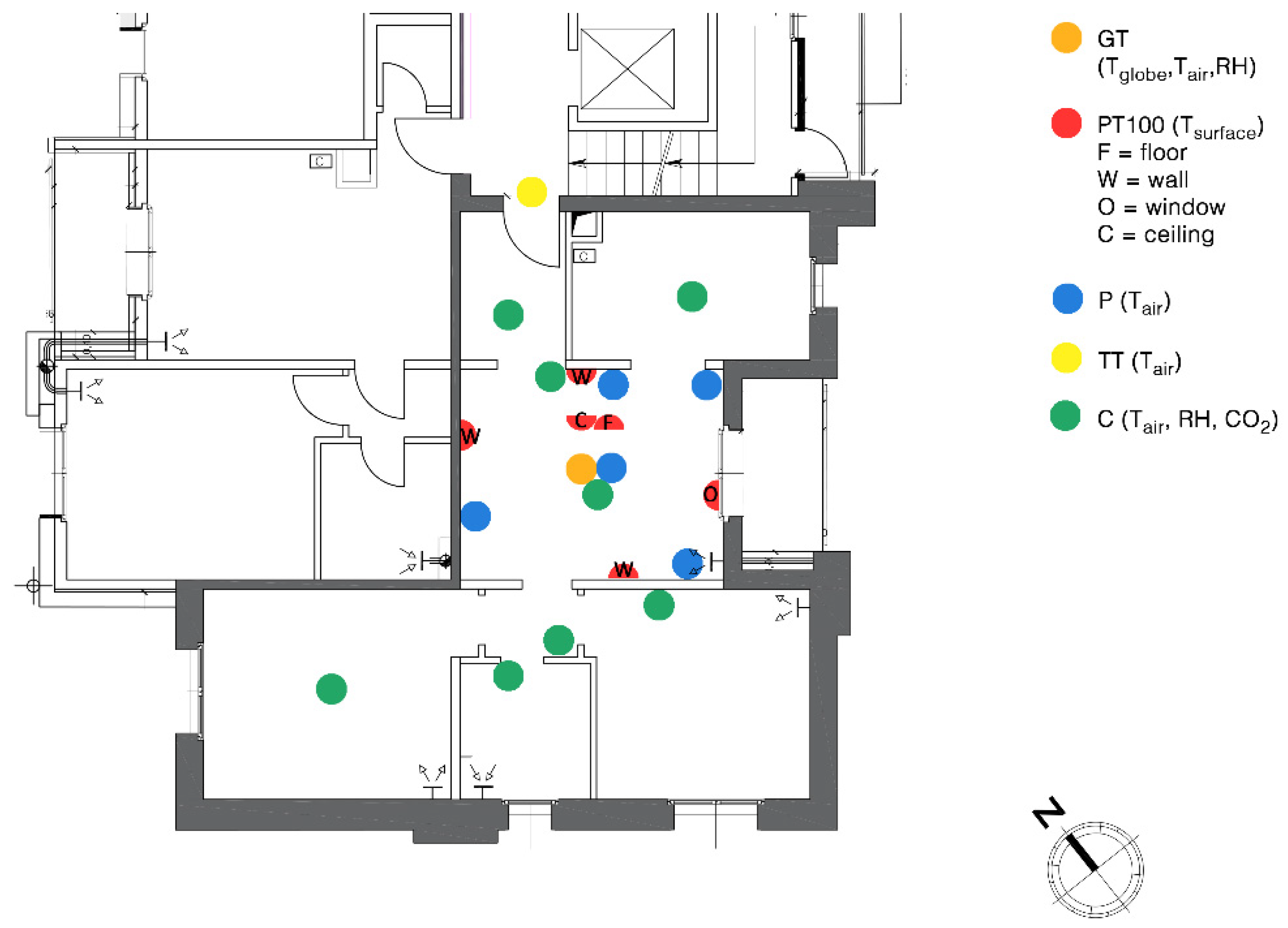
Table 5. Sensors’ specifications.
SensorsCode in Figure 3Measured
Quantities
AccuracyResolution
Capetti
(mod. WSD20TH2CO)
CAir temperature,
Relative humidity,
CO2 concentration
T: ± 0.2 °C
HR: ± 2.0%
CO2:
0 ÷ 2000 ppm: < ± 50 ppm
0 ÷ 5000 ppm: < ± 50 ppm
0 ÷ 10,000 ppm: < ± 100 ppm
T: 0.01 °C
HR: 0.05%RH
CO2: 1 ppm
Capetti (mod. WSS00T)PAir temperature±0.2 °C0.01 °C
Pt100 (mod. ESU403.1)W(wall); F(floor);
C(ceiling); O(window)
Surface temperature±0.1 °C0.01 °C
Globe-thermometer output Pt100–LSI (mod. EST131)
[emissivity: 0.95; diameter: 15 cm]
GTGlobe-thermometric temperature±0.15 °C0.01 °C
Tinytag (mod. TGU-4500)TTAir temperatureT: ±0.2 °C (for T: −10 ÷ 30 °C)0.01 °C
Table 6. Flexibility tests carried out during the winter season over the years 2020 and 2021.
ID TestChargeLoad-Shifting
Δtc
[Day]
Δt EN 16798–1:2019
(Δt TS) [Day]
Ti
[°C]
Tmin
[°C]
ΔTAfter 1 day [°C]ΔTAfter 2 days [°C]ΔTAfter 3 days [°C]Tout Avg (min; max) [°C]
F2_20_22.94.0 * (4.0)26.120.63.54.64.86.9 (2.1; 14)
F2_20_41.24.0 (4.8)24.019.52.92.63.58.1 (1.9; 18.9)
F2_20_50.41.4 (1.4)22.519.52.0--8.1 (2.4; 16.6)
F3_20_25.13.5 * (6.9)25.119.52.73.94.79.2 (3.4; 16.9)
F3_20_32.11.0 (3.9)21.519.11.42.02.311 (5.2; 20.2)
F2_21_11.22.3 * (2.3)26.220.83.55.0-7.6 (0.6; 14.3)
F2_21_20.64.3 (4.3)23.820.22.52.93.312.1 (4.8; 21.1)
F2_21_31.35.3 * (5.3)27.723.13.23.84.110.6 (4.8; 18.4)
F3_21_14.84.2 (4.2)24.320.72.02.93.47.7 (1.6; 12.9)
F3_21_21.23.1 * (3.1)24.820.32.73.64.52.2 (−2.4; 7.1)
F3_21_30.73.1 * (3.1)26.121.33.64.34.88.7 (5.9; 14.3)
F3_21_41.33.8 * (3.8)28.322.93.84.75.211.4 (5.5; 21)
F3_21_50.64.2 * (4.2)26.822.23.13.84.110.6 (4.8; 18.4)
F2_22_22.32.2 (2.2)23.020.41.82.45.2 (0.5; 11.4)
F2_22_30.91.2 (3.6)23.419.12.33.44.12.2 (−2.7; 6.9)
F2_22_42.01.5 (2.5)22.919.92.93.05.9 (−0.6; 15.7)
F2_22_54.38.3 (8.5)22.719.81.11.31.57.8 (0.6; 15)
F2_22_62.30.7 (3.5)23.019.83.33.03.7 (0.5; 9)
F2_22_71.02.6 (2.6)23.121.40.81.19.5 (5.4; 15.2)
F2_22_80.37.4 (8.7)23.119.61.10.91.18.8 (−0.3; 19)
F2_22_90.61.8 (3.3)22.419.62.12.42.88.5 (4.1; 15.1)
F2_22_101.45.0 (10.0)23.219.72.42.82.89.1 (−1; 16.5)
F2_22_111.311.0 (11.0)24.323.00.20.10.211.9 (3.9; 24)
F3_22_34.01.1 (2.1)23.119.42.83.75.1 (0.5; 11.4)
F3_22_42.10.8 (4.5)23.017.13.14.21.9 (−2.7; 6.6)
F3_22_53.01.0 (1.9)23.019.52.93.38.6 (2.9; 15.7)
F3_22_62.12.0 (8)22.918.32.12.83.46.8 (1.9; 13.8)
F3_22_73.00.7 (3.5)23.218.23.54.34.43.7 (0.5; 9)
F3_22_90.30.4 (8.8)22.018.11.92.02.18.7 (−0.3; 19)
F3_22_102.00.9 (3.5)22.218.92.22.83.16.6 (−1; 16.1)
F3_22_111.311.0 (11.0)23.521.50.50.71.112 (3.9; 24)
* In these tests, the upper limit of comfort was exceeded (thus, the first part of the discharging phase is outside the comfort range) in order to evaluate the impact of different initial temperatures of discharge, and possible applications in buildings unoccupied during a certain period of the day or the week.
Publisher’s Note: MDPI stays neutral with regard to jurisdictional claims in published maps and institutional affiliations.

